Model Based Optimal Control, Estimation, and ... - Scott Moura

Electronic Theses and Dissertations UC Berkeley Peer Reviewed Title: Model Based Optimal Control, Estimation, and Validation of Lithium-Ion Batteries Author: Perez, Hector Eduardo Acceptance Date: 2016 Series: UC Berkeley Electronic Theses and Dissertations Degree: Ph.D., Civil and Environmental EngineeringUC Berkeley Advisor(s): Moura, Scott J Committee: Sengupta, Raja, Callaway, Duncan S Permalink: http://escholarship.org/uc/item/7mm747m8 Abstract: Copyright Information: All rights reserved unless otherwise indicated. Contact the author or original publisher for any necessary permissions. eScholarship is not the copyright owner for deposited works. Learn more at http://www.escholarship.org/help_copyright.html#reuse

eScholarship provides open access, scholarly publishing services to the University of California and delivers a dynamic research platform to scholars worldwide.

Model Based Optimal Control, Estimation, and Validation of Lithium-Ion Batteries by Hector Eduardo Perez

A dissertation submitted in partial satisfaction of the requirements for the degree of Doctor of Philosophy in Engineering - Civil and Environmental Engineering in the Graduate Division of the University of California, Berkeley

Committee in charge: Assistant Professor Scott J. Moura, Chair Professor Raja Sengupta Associate Professor Duncan S. Callaway Summer 2016

Model Based Optimal Control, Estimation, and Validation of Lithium-Ion Batteries

Copyright 2016 by Hector Eduardo Perez

1 Abstract

Model Based Optimal Control, Estimation, and Validation of Lithium-Ion Batteries by Hector Eduardo Perez Doctor of Philosophy in Engineering - Civil and Environmental Engineering University of California, Berkeley Assistant Professor Scott J. Moura, Chair This dissertation focuses on developing and experimentally validating model based control techniques to enhance the operation of lithium ion batteries, safely. An overview of the contributions to address the challenges that arise are provided below. Chapter 1: This chapter provides an introduction to battery fundamentals, models, and control and estimation techniques. Additionally, it provides motivation for the contributions of this dissertation. Chapter 2: This chapter examines reference governor (RG) methods for satisfying state constraints in Li-ion batteries. Mathematically, these constraints are formulated from a first principles electrochemical model. Consequently, the constraints explicitly model specific degradation mechanisms, such as lithium plating, lithium depletion, and overheating. This contrasts with the present paradigm of limiting measured voltage, current, and/or temperature. The critical challenges, however, are that (i) the electrochemical states evolve according to a system of nonlinear partial differential equations, and (ii) the states are not physically measurable. Assuming available state and parameter estimates, this chapter develops RGs for electrochemical battery models. The results demonstrate how electrochemical model state information can be utilized to ensure safe operation, while simultaneously enhancing energy capacity, power, and charge speeds in Li-ion batteries. Chapter 3: Complex multi-partial differential equation (PDE) electrochemical battery models are characterized by parameters that are often difficult to measure or identify. This parametric uncertainty influences the state estimates of electrochemical model-based observers for applications such as state-of-charge (SOC) estimation. This chapter develops two sensitivity-based interval observers that map bounded parameter uncertainty to state estimation intervals, within the context of electrochemical PDE models and SOC estimation. Theoretically, this chapter extends the notion of interval observers to PDE models using a sensitivity-based approach. Practically, this chapter quantifies the sensitivity of battery state estimates to parameter variations, enabling robust battery management schemes. The effectiveness of the proposed sensitivity-based interval observers is verified via a numerical study for the range of uncertain parameters.

2 Chapter 4: This chapter seeks to derive insight on battery charging control using electrochemistry models. Directly using full order complex multi-partial differential equation (PDE) electrochemical battery models is difficult and sometimes impossible to implement. This chapter develops an approach for obtaining optimal charge control schemes, while ensuring safety through constraint satisfaction. An optimal charge control problem is mathematically formulated via a coupled reduced order electrochemical-thermal model which conserves key electrochemical and thermal state information. The Legendre-Gauss-Radau (LGR) pseudo-spectral method with adaptive multi-mesh-interval collocation is employed to solve the resulting nonlinear multi-state optimal control problem. Minimum time charge protocols are analyzed in detail subject to solid and electrolyte phase concentration constraints, as well as temperature constraints. The optimization scheme is examined using different input current bounds, and an insight on battery design for fast charging is provided. Experimental results are provided to compare the tradeoffs between an electrochemical-thermal model based optimal charge protocol and a traditional charge protocol. Chapter 5: Fast and safe charging protocols are crucial for enhancing the practicality of batteries, especially for mobile applications such as smartphones and electric vehicles. This chapter proposes an innovative approach to devising optimally health-conscious fast-safe charge protocols. A multi-objective optimal control problem is mathematically formulated via a coupled electro-thermal-aging battery model, where electrical and aging sub-models depend upon the core temperature captured by a two-state thermal sub-model. The LegendreGauss-Radau (LGR) pseudo-spectral method with adaptive multi-mesh-interval collocation is employed to solve the resulting highly nonlinear six-state optimal control problem. Charge time and health degradation are therefore optimally traded off, subject to both electrical and thermal constraints. Minimum-time, minimum-aging, and balanced charge scenarios are examined in detail. Sensitivities to the upper voltage bound, ambient temperature, and cooling convection resistance are investigated as well. Experimental results are provided to compare the tradeoffs between a balanced and traditional charge protocol. Chapter 6: This chapter provides concluding remarks on the findings of this dissertation and a discussion of future work.

i

To My Parents Who have instilled in me the values to make this all possible.

ii

Contents Contents

ii

List of Figures

iv

List of Tables

viii

1 Introduction 1.1 Battery System Overview . . . . . . . 1.2 Battery Fundamentals . . . . . . . . . 1.3 Battery Models . . . . . . . . . . . . . 1.4 Battery Control and Estimation . . . . 1.5 Challenges . . . . . . . . . . . . . . . . 1.6 New Contributions of this Dissertation 1.7 Organization . . . . . . . . . . . . . .

. . . . . . .

. . . . . . .

. . . . . . .

. . . . . . .

. . . . . . .

. . . . . . .

. . . . . . .

. . . . . . .

. . . . . . .

. . . . . . .

. . . . . . .

. . . . . . .

. . . . . . .

. . . . . . .

. . . . . . .

. . . . . . .

. . . . . . .

2 Enhanced Performance of Li-ion Batteries via Modified Reference ernors & Electrochemical Models 2.1 Introduction . . . . . . . . . . . . . . . . . . . . . . . . . . . . . . . . 2.2 Electrochemical Model & Motivation . . . . . . . . . . . . . . . . . . 2.3 Modified Reference Governor (MRG) Designs . . . . . . . . . . . . . 2.4 Numerical Results . . . . . . . . . . . . . . . . . . . . . . . . . . . . . 2.5 Conclusions . . . . . . . . . . . . . . . . . . . . . . . . . . . . . . . . 3 Sensitivity-Based Interval PDE Observers for Estimation 3.1 Introduction . . . . . . . . . . . . . . . . . . . 3.2 Electrochemical Model Development . . . . . 3.3 Backstepping PDE Observer Design . . . . . . 3.4 Observer Sensitivity Equations . . . . . . . . . 3.5 Sensitivity-based Interval Observers . . . . . . 3.6 Simulations . . . . . . . . . . . . . . . . . . . 3.7 Conclusions . . . . . . . . . . . . . . . . . . .

. . . . . . .

. . . . . . .

. . . . . . .

. . . . . . .

1 3 4 5 6 8 8 9

Gov. . . . .

. . . . .

. . . . .

. . . . .

10 10 12 14 18 26

Lithium-Ion Battery SOC . . . . . . .

. . . . . . .

. . . . . . .

. . . . . . .

. . . . . . .

. . . . . . .

. . . . . . .

. . . . . . .

. . . . . . .

. . . . . . .

. . . . . . .

. . . . . . .

. . . . . . .

. . . . . . .

. . . . . . .

. . . . . . .

. . . . . . .

28 28 30 34 34 37 39 45

iii 4 Optimal Charging of Li-Ion Batteries via a Single Particle Model with Electrolyte and Thermal Dynamics 4.1 Introduction . . . . . . . . . . . . . . . . . . . . . . . . . . . . . . . . . . . . 4.2 Single Particle Model with Electrolyte and Thermal Dynamics . . . . . . . . 4.3 Optimal Charge Control Formulation . . . . . . . . . . . . . . . . . . . . . . 4.4 Results and Discussion . . . . . . . . . . . . . . . . . . . . . . . . . . . . . . 4.5 Experimental Results and Discussion . . . . . . . . . . . . . . . . . . . . . . 4.6 Conclusions . . . . . . . . . . . . . . . . . . . . . . . . . . . . . . . . . . . .

46 46 48 52 53 56 60

5 Optimal Charging of Li-Ion Batteries with Aging Dynamics 5.1 Introduction . . . . . . . . . . . . . . . . . . 5.2 Coupled Electro-Thermal-Aging Model . . . 5.3 Formulation of Optimal Charge Control . . . 5.4 Optimization Results and Discussion . . . . 5.5 Experimental Results and Discussion . . . . 5.6 Conclusions . . . . . . . . . . . . . . . . . .

. . . . . .

62 62 64 68 70 77 79

6 Conclusion 6.1 Contributions . . . . . . . . . . . . . . . . . . . . . . . . . . . . . . . . . . . 6.2 Future Work Opportunities . . . . . . . . . . . . . . . . . . . . . . . . . . .

80 80 81

Bibliography

83

A Nomenclature

91

B Pseudo-Spectral Optimal Control

99

C Battery in the Loop Test System

102

Coupled Electro-Thermal. . . . . .

. . . . . .

. . . . . .

. . . . . .

. . . . . .

. . . . . .

. . . . . .

. . . . . .

. . . . . .

. . . . . .

. . . . . .

. . . . . .

. . . . . .

. . . . . .

. . . . . .

. . . . . .

. . . . . .

iv

List of Figures 1.1 1.2 1.3 1.4 1.5 1.6 1.7 1.8 2.1

2.2

2.3

2.4 2.5

2.6

Battery Cell Failure in a Samsung Galaxy S3 Smart Phone, adopted from [1] . . Battery Pack Failure in a Boeing 787 Commercial Airplane, adopted from [2] . . Left: A123 26650 2.3Ah Cylindrical Cell, adopted from [3]. Right: A123 AMP20 20Ah Prismatic Cell, adopted from [3]. . . . . . . . . . . . . . . . . . . . . . . . 2016 Chevrolet Malibu HEV 1.5kWh Battery Pack, adopted from [4] . . . . . . Cylindrical Cell Construction, adopted from [5] . . . . . . . . . . . . . . . . . . Electrochemical Cell Cross Section . . . . . . . . . . . . . . . . . . . . . . . . . Overview of Battery Models . . . . . . . . . . . . . . . . . . . . . . . . . . . . . Operation Limits Comparison . . . . . . . . . . . . . . . . . . . . . . . . . . . . Schematic of the Doyle-Fuller-Newman model [6]. The model considers two phases: the solid and electrolyte. In the solid, states evolve in the x and r dimensions. In the electrolyte, states evolve in the x dimension only. The cell is divided into three regions: anode, separator, and cathode. . . . . . . . . . . . . Motivating example of Li plating. Evolution of current I(t), reference current I r (t), and side reaction overpotential ηs (L− , t) for a 10sec 3C pulse charging scenario, with and without a modified reference governor. . . . . . . . . . . . . . Motivating example of lithium depletion in the electrolyte. The model is invalid after ce (0+ , t) < 0. Evolution of current I(t), reference current I r (t), and electrolyte concentration ce (0+ , t) for a 10sec 7C pulse discharging scenario, with and without a modified reference governor. . . . . . . . . . . . . . . . . . . . . . . . Block diagram of modified reference governor with direct measurements of the constrained variables y. . . . . . . . . . . . . . . . . . . . . . . . . . . . . . . . . Comparison of CCCV and modified reference governor (MRG) charging. The MRG regulates ηs near its limit, thereby achieving 95% SOC in 14.9min vs. 35.5min for CCCV by allowing voltage to safely exceed 4.2V. . . . . . . . . . . . Comparison of MRG and LMRG. Signals include current I(t), reference current I r (t), and side reaction overpotential ηs (L− , t) for a 10sec 3C pulse charging scenario. The LMRG does not reach the constraint, due to linearization modeling errors. . . . . . . . . . . . . . . . . . . . . . . . . . . . . . . . . . . . . . . . . .

2 2 3 3 4 5 7 7

11

14

15 15

18

19

v 2.7

Comparison of MRG and LMRG. Signals include current I(t), reference current I r (t), and electrolyte concentration ce (0+ , t) for a 10sec 7C pulse discharging scenario. The LMRG violates the constraint, due to linearization modeling errors. 2.8 US06x3 1.4I VO: Left: Reference Current I r (t) and Current I(t), Voltage V (t), State of Charge SOC(t), Temperature T (t). Right: Side Reaction Overpotential ηs (L− , t), Electrolyte Concentration ce (0+ , t), ce (0− , t), Surface Concentrations θ(0− , t), θ(L− , t), θ(0+ , t), θ(L+ , t). . . . . . . . . . . . . . . . . . . . . . . . 2.9 US06x3 (1.4I) MRG. Left: Reference Current I r (t) and Current I(t), Voltage V (t), State of Charge SOC(t), Temperature T (t). Right: β(t), Side Reaction Overpotential ηs (L− , t), Electrolyte Concentration ce (0+ , t), ce (0− , t), Surface Concentrations θ(0− , t), θ(L− , t), θ(0+ , t), θ(L+ , t). . . . . . . . . . . . . . . . . . 2.10 Temperature vs. Voltage operating points for (a) 1.0I, (b) 1.2I, and (c) 1.4I over US06x3 cycle. . . . . . . . . . . . . . . . . . . . . . . . . . . . . . . . . . . . . . 2.11 US06x3 power responses for (a) 1.0I, (b) 1.2I, and (c) 1.4I. . . . . . . . . . . . . 2.12 US06x3 Power Histogram for (a) 1.0I, (b) 1.2I, and (c) 1.4I. . . . . . . . . . . . 3.1 3.2

3.3 3.4 3.5

3.6 3.7 3.8 3.9 3.10 3.11 3.12 3.13

Each electrode is idealized as a single porous spherical particle. This model results from assuming the electrolyte concentration is constant in space and time [7]. . Block diagram of estimation scheme where the boundary state error is injected into the estimator. The use of the boundary state c− ss is determined by ϕ(V, I), which inverts the nonlinear output w.r.t. the state, uniformly in the input current. The double spatial derivative estimates cˆ− srr (r, t) along with input current I(t) and output inversion ϕ(V, I) are fed into the sensitivity PDEs. The sensitivity estimates S1 (r, t), S2 (r, t), S3 (r, t), S4 (r, t), spatial derivatives of the sensitivity estimates S1r (r, t), S2r (r, t), S3r (r, t), S4r (r, t), and the concentration estimates ˆ− cˆ− c− s (r, t)H,A , cs (r, t)H,A . . . . . . . s are used to calculate the interval estimates ˆ Pulse Charge/Discharge Cycle (a) Input current. (b) Sensitivity. (c) Bulk SOC. (d) Output Voltage. . . . . . . . . . . . . . . . . . . . . . . . . . . . . . . . . . UDDSx2 Charge/Discharge Cycle (a) Input current. (b) Sensitivity. (c) Bulk SOC. (d) Output Voltage. . . . . . . . . . . . . . . . . . . . . . . . . . . . . . . Normalized parameter sensitivity ranking (average in blue, standard deviation in red) across various electric vehicle-like charge/discharge cycles (UDDSx2, US06x3, SC04x4, LA92x2, DC1, DC2). . . . . . . . . . . . . . . . . . . . . . . . . . . . . Pulse Charge/Discharge Cycle SOC Trajectories for ε = {0.9, 0.95, 1.0, 1.05, 1.1}. Pulse Charge/Discharge Cycle Voltage Trajectories for ε = {0.9, 0.95, 1.0, 1.05, 1.1}. Pulse Charge/Discharge Cycle SOC Trajectories for q = {0.9, 0.95, 1.0, 1.05, 1.1}. Pulse Charge/Discharge Cycle Voltage Trajectories for q = {0.9, 0.95, 1.0, 1.05, 1.1}. Pulse Charge/Discharge Cycle SOC Trajectories for γ = {0.9, 0.95, 1.0, 1.05, 1.1}. Pulse Charge/Discharge Cycle Voltage Trajectories for γ = {0.9, 0.95, 1.0, 1.05, 1.1}. Pulse Charge/Discharge Cycle SOC Trajectories for δ = {0.6, 0.9, 1.0, 1.1, 1.4}. . Pulse Charge/Discharge Cycle Voltage Trajectories for δ = {0.6, 0.9, 1.0, 1.1, 1.4}.

20

21

22 23 24 25 30

33 40 40

42 43 43 43 43 44 44 44 44

vi 4.1

Each electrode is idealized as a single porous spherical particle whose dynamics evolve in the r dimension. The electrolyte concentration dynamics evolve in all regions in the x dimension. . . . . . . . . . . . . . . . . . . . . . . . . . . . . . . − 4.2 Block diagram of SPMeT. Note that the c+ s , cs , ce subsystems are independent of one another. However, all subsystems are coupled through temperature since it − feeds back into the nonlinear voltage output and c+ s , cs , ce subsystems. . . . . . 4.3 Minimum time charge results with Imax = {8.5C, 7.25C, 6C}. Left: Current I(t), Voltage V (t), State of Charge SOC(t), Temperatures Tc (t), Ts (t). Right: Surface − + + Concentrations θ− (t), θ+ (t), Electrolyte Concentrations c− e (0 , t), ce (0 , t). . . . 4.4 Optimized charge vs. CC-CV charge trajectories with Imax = 6C. Left: Current I(t), Voltage V (t), State of Charge SOC(t), Temperatures Tc (t), Ts (t). Right: − + + Surface Concentrations θ− (t), θ+ (t), Electrolyte Concentrations c− e (0 , t), ce (0 , t). 4.5 Influence of a ±2.5% deviation in De (ce , Tavg ) on optimization results for minimum time charge with Imax = 8.5C. Left: Current I(t), Voltage V (t), State of Charge SOC(t), Temperatures Tc (t), Ts (t). Right: Surface Concentrations − + + θ− (t), θ+ (t), Electrolyte Concentrations c− e (0 , t), ce (0 , t). . . . . . . . . . . . . 4.6 Experimental Determination of Open Circuit Potentials from Open Circuit Voltage: Estimated Open Circuit Voltage (U + (θ+ )−(U − (θ− ))Est , Experimental Open Circuit Voltage (U + (θ+ ) − U − (θ− ))Exp , Cathode Open Circuit Potential U + (θ+ ), and Anode Open Circuit Potential U − (θ− ). . . . . . . . . . . . . . . . . . . . . 4.7 Experimental Validation of Electrochemical-Thermal Model via SPMeT Optimal Charge Protocol when Imax = 8.5C: Current I(t), Model Voltage V (t)SP M eT , Experimental Voltage V (t)Exp , Model Temperatures Tc (t)SP M eT , Ts (t)SP M eT , and Experimental Temperature Ts (t)Exp . . . . . . . . . . . . . . . . . . . . . . . . . 4.8 Experimental Validation of Electrochemical-Thermal Model via SPMeT Optimal Charge Protocol when Imax = 7.25C: Current I(t), Model Voltage V (t)SP M eT , Experimental Voltage V (t)Exp , Model Temperatures Tc (t)SP M eT , Ts (t)SP M eT , and Experimental Temperature Ts (t)Exp . . . . . . . . . . . . . . . . . . . . . . . . . 4.9 Experimental Validation of Electrochemical-Thermal Model via SPMeT Optimal Charge Protocol when Imax = 6C: Current I(t), Model Voltage V (t)SP M eT , Experimental Voltage V (t)Exp , Model Temperatures Tc (t)SP M eT , Ts (t)SP M eT , and Experimental Temperature Ts (t)Exp . . . . . . . . . . . . . . . . . . . . . . . . . 4.10 SPMeT Optimal Charge with Imax = 6C (Open Loop) and 5C CC-CV Charge Protocol (Closed Loop) Aging: Capacity Fade, and Charge Time. . . . . . . . . 5.1 5.2 5.3 5.4 5.5

Schematic of the Electrical Model. . . . . . . . . . . . . . . . . . . . . . . . . . Electrical Parameters for Charge identified in [8, 9]: (a) Voc , (b) R0 , (c) C1 , (d) R1 , (e) C2 , and (f) R2 . . . . . . . . . . . . . . . . . . . . . . . . . . . . . . . . . Schematic of the Thermal Model (adopted from [9]). . . . . . . . . . . . . . . . Battery SOH Model: (a) EOL Cycle N (c, Tc ), and (b) SOH Decay Rate as Functions of C-rate. . . . . . . . . . . . . . . . . . . . . . . . . . . . . . . . . . . . . Electro-Thermal-Aging Model Coupling. . . . . . . . . . . . . . . . . . . . . . .

48

49

53

54

55

57

58

58

59 60 64 65 66 67 69

vii 5.6 5.7 5.8 5.9 5.10 5.11 5.12 5.13 5.14 5.15 5.16 5.17

Optimization Result for the Minimum-Time Charge: (a) C-rate, (b) Terminal Voltage, (c) Core and Surface Temperatures, and (d) SOC/SOH. . . . . . . . . Comparison with CCCV Charge: (a) C-rate, (b) Core Temperature, and (c) SOC. Optimization Result for the Minimum-Aging Charge: (a) C-rate, (b) Terminal Voltage, (c) Core and Surface Temperatures, and (d) SOC/SOH. . . . . . . . . SOH Trajectories of the Minimum-Aging Charge and C/10 CCCV Charge. . . . Pareto Curve, Charge Time Versus SOH Decay. . . . . . . . . . . . . . . . . . . Optimization Result for the Balanced Charge (β = 0.34): (a) C-rate, (b) Terminal Voltage, (c) Core and Surface Temperatures, and (d) SOC/SOH. . . . . . . . . Trajectory of the Total Equivalent Resistance (R0 +R1 +R2 ) for Balanced Charge (β = 0.34). . . . . . . . . . . . . . . . . . . . . . . . . . . . . . . . . . . . . . . Influence of Vt,max on Pareto Curve. . . . . . . . . . . . . . . . . . . . . . . . . . Influence of Tf on Pareto Curve. . . . . . . . . . . . . . . . . . . . . . . . . . . Influence of Ru on Pareto Curve. . . . . . . . . . . . . . . . . . . . . . . . . . . Experimental Validation of Electro-Thermal Model via Balanced Charge Protocol: (a) Terminal Voltage, and (b) Temperature. . . . . . . . . . . . . . . . . . . Balanced and 5C CCCV Charge Protocol Aging: (a) Capacity Fade, and (b) Charge Time. . . . . . . . . . . . . . . . . . . . . . . . . . . . . . . . . . . . . .

6.1 6.2

Electrochemical Model Based Control Diagram - Closed Loop . . . . . . . . . . Equivalent Circuit Model Based Control Diagram - Closed Loop . . . . . . . . .

C.1 C.2 C.3 C.4

Battery in the Loop Test System Diagram . . . . Battery Cell Setup in Environmental Chamber . . Battery Cell Setup in Cell Holder . . . . . . . . . Fault Inducing Battery Cell Setup in Cell Holder

. . . .

. . . .

. . . .

. . . .

. . . .

. . . .

. . . .

. . . .

. . . .

. . . .

. . . .

. . . .

. . . .

. . . .

. . . .

. . . .

. . . .

71 71 72 72 73 74 74 75 75 76 77 78 82 82 102 103 104 105

viii

List of Tables 2.1 2.2 2.3

CPU Time per Simulated Time for Nonlinear and Linear MRGs. . . . . . . . . . Mean power benefits of using MRG vs. VO. . . . . . . . . . . . . . . . . . . . . Energy benefits of using MRG vs. VO. . . . . . . . . . . . . . . . . . . . . . . .

20 26 26

4.1

Minimum Charge Times for Perturbed Solutions. . . . . . . . . . . . . . . . . .

56

5.1 5.2

Thermal Parameters. . . . . . . . . . . . . . . . . . . . . . . . . . . . . . . . . . Pre-Exponential Factor as a Function of the C-Rate. . . . . . . . . . . . . . . .

66 68

A.1 A.2 A.3 A.4

Nomenclature: Nomenclature: Nomenclature: Nomenclature:

92 94 96 98

Chapter Chapter Chapter Chapter

2 3 4 5

. . . .

. . . .

. . . .

. . . .

. . . .

. . . .

. . . .

. . . .

. . . .

. . . .

. . . .

. . . .

. . . .

. . . .

. . . .

. . . .

. . . .

. . . .

. . . .

. . . .

. . . .

. . . .

. . . .

. . . .

. . . .

. . . .

. . . .

. . . .

. . . .

. . . .

ix

Acknowledgments I would like to start by thanking all of those that have been around me for making these past three years of my doctoral studies and research possible. I have not only received the well needed support from friends and family, but from fellow students, staff, administrators, and faculty members as well. I am very proud to have been given the opportunity to sharpen my theoretical and experimental skills while providing guidance and mentorship to multiple undergraduate student projects throughout my stay. This work would not be possible without the help of my long time mentor and research advisor Assistant Professor Scott Moura for believing in and advocating for me to join the University of California, Berkeley at the beginning of his career as a tenure track professor in 2013. For many years now, he has been a source of inspiration for obtaining graduate degrees. I initially met him at a GEM Grad Lab at the 2008 Society of Hispanic Professional Engineers (SHPE) National Conference when I was an undergraduate student at the California State University, Northridge (CSUN) and he a doctoral student at the University of Michigan (UofM). That led me to graduate studies at UofM, where I obtained a Master of Science degree in 2012. His continued mentorship and interest in my success motivated me to join him for the pursuit of my doctoral degree in 2013. His advice and push for technical excellence in the classroom and the research environment has enabled me to excel in ways I never thought possible, all while building a world class battery in the loop test facility that will enable the development, integration, and validation of advanced battery management technologies in the years to come. It has been an amazing experience to see the Energy, Controls, and Applications Lab (eCAL) grow into what it is today. This dissertation would not be possible without the close advice from Dr. Satadru Dey and Dr. Xiaosong Hu. Their advice has been instrumental to the development of the contents in this dissertation. This work would not be what it is without the help from my labmates Eric Burger, Eric Munsing, Caroline Le Floch, Saehong Park, Dong Zhang, and Hongcai Zhang. I thank them for the help they have provided me through individual discussions, and lab team meetings. I would also like to express gratitude to the undergraduate students I have mentored at eCAL for supporting various battery related works: Loan Kim, Niloofar Shahmohammadhamedani, Khajag Geukjian, Defne Gun, Othmane Benkirane, Ibrahim Youssef, and Preet Gill. I am also very grateful for and thank those who have been co-authors of my work. I would also like to thank Associate Professor Duncan Callaway and Professor Raja Sengupta for being part of my dissertation committee, and giving me feedback on this work. Additionally, I would like to thank Prof. Anna Stefanopoulou, Dr. Jason Siegel, and Dr. Xinfan Lin, colleagues at the University of Michigan and the Ford Motor Company for providing useful insight for my doctoral work during our talks at conferences. I am also very thankful for the opportunities that the College of Engineering has granted me to fulfill my extracurricular endeavors including the opportunity to co-found and lead the first ever Bay Area Graduate Pathways Symposium (GPS) graduate outreach event to inspire diverse talent to become the next generation of innovative leaders through advanced

x engineering degrees. I thank the graduate student committee (William Tarpeh, Christina Fuentes, Maribel Jaquez, Allan Ogwang, Regan Patterson, Raj Kumar, and Karina Chavarria) for their dedication to making this event a success. Additionally, I thank Meltem Erol, and Associate Dean for Equity & Inclusion and Student Affairs Prof. Oscar Dubon for believing in my vision and providing support to making Bay Area GPS a reality. The financial support necessary to complete my doctoral education and this work was made possible by the Ford Foundation as a Predoctoral Fellow, the Graduate Division, the Special State Fund for Strategic Research Grant, the Civil and Environmental Engineering Department, and the Energy, Controls, and Applications Lab. I thank all of these sources for allowing me to focus on my doctoral studies and research throughout my stay. I am lucky to have found Maribel Jaquez a few years ago here at Berkeley during a graduate social event. We became close friends by conversing about things that we like in common such as good Mexican food and outreach. I thank my loving girlfriend of a little over two years for being extremely supportive in addressing the many challenges that have come my way. Finally, I would like to thank my parents Francisco and Teresita Perez for their endless love and support throughout my doctoral studies at the University of California, Berkeley. They have been a great influence to me and I am very proud to dedicate this dissertation to them. Their hard work and dedication to my success as a first generation graduate of any formal education have given me the confidence needed to achieve anything that comes my way.

1

Chapter 1 Introduction Battery systems are an enabling technology as we progress towards an electrified future that ranges from mobile devices such as smart phones to electrified transportation. There are currently around 7.4 billion active mobile subscriptions around the globe [10]. The Electric Vehicles Initiative (EVI), a multi-government initiative to accelerate the adoption of electric vehicles (EVs) worldwide aims for 20 million EVs including plug in electric vehicles (PHEVs) and fuel cell electric vehicles (FCVs) by the year 2020 [11]. The pressing needs of battery technologies are apparent based on cost and energy targets despite their respective decrease and increase over the past few years [11]. Even though these technologies have advanced, the growing needs of our society call for rapid charging and increased performance of batteries. To accomplish this, better batteries can be made through the development of new materials or higher performance can be obtained from existing (or new) batteries through controls & estimation advances. This work focuses on the latter to enhance the operation of lithium ion batteries with respect to charge time, power, energy, and life, safely. As battery technologies mature, careful control strategies are required to ensure safety. Figure 1.1-1.2, show lithium ion batteries that exploded in a smart phone and a commercial airplane, respectively. The damage possible from the misuse of these batteries is apparent, and it is clear that safety is extremely important for the proliferation of battery technologies. The model based techniques discussed in this dissertation aim to address some of the challenges that arise when achieving the highest performance physically possible from lithium ion batteries within a safe operating window. The rest of this chapter gives an overview of battery systems, fundamentals, models, controls and estimation, and organization of the dissertation.

CHAPTER 1. INTRODUCTION

2

Figure 1.1: Battery Cell Failure in a Samsung Galaxy S3 Smart Phone, adopted from [1]

Figure 1.2: Battery Pack Failure in a Boeing 787 Commercial Airplane, adopted from [2]


3

Figure 1.3: Left: A123 26650 2.3Ah Cylindrical Cell, adopted from [3]. Right: A123 AMP20 20Ah Prismatic Cell, adopted from [3].

Figure 1.4: 2016 Chevrolet Malibu HEV 1.5kWh Battery Pack, adopted from [4]

1.1

Battery System Overview

Commercial lithium ion battery cells usually are usually packaged in two forms, cylindrical and prismatic (shown in Fig. 1.3). The operating voltage of a single cell for various lithium ion battery chemistries is typically between 2 and 4.2 volts. For applications requiring higher voltages and energy/power capacities, battery cells are connected in series and parallel to form a battery pack with the desired voltage and energy/power. A battery pack composed of multiple cells for an HEV is shown Fig. 1.4. The battery pack also consists of various sensors (current, voltage, and temperature) which are connected to a battery management system (BMS) which manages its operation (eg. charging, discharging, etc.). This dissertation develops and validates model based techniques which are meant to occur within the BMS.


4

Aluminum Foil Cathode Separator Anode Copper Foil

Figure 1.5: Cylindrical Cell Construction, adopted from [5]

1.2

Battery Fundamentals

The typical construction of a spirally wound cylindrical battery cell is shown in Fig. 1.5. The copper foil typically serves as the current collector for the negative electrode known as the anode (which contains the active material), which is attached to the negative terminal of the cell. The separator is an electrical insulator which allows lithium ions to flow from the anode to the cathode (and vice versa), while ensuring electrons flow external to the cell. The aluminum foil typically serves as the current collector for the positive electrode known as the cathode (which contains the active material), which is attached to the positive terminal of the cell. This electrode assembly is rolled up into a jelly roll, and then inserted into a cylindrical can (with current collectors attached to the terminals of the cell). The electrolyte is then inserted (which flows through the porous electrodes and separator assembly) and the can is sealed. A similar process is followed to form prismatic cells which use stacked or folded electrode assembly designs to form a cell. A cross section of an electrode assembly is shown in Fig. 1.6 to understand the operation of a lithium ion battery. When fully charged, the majority of the lithium in the cell exists within the solid phase particles in the anode, typically lithiated carbon Lix C6 , that are idealized as symmetric spherical particles. Under discharge, the lithium diffuses from the interior to the surface of the spherical particles in the anode. An electrochemical reaction at the surface separates the lithium into a positive lithium ion and electron as Lix C6 C6 + xLi+ + xe− .

(1.1)

The lithium ion then migrates from the anode through the separator and into the cathode. The corresponding electron then travels through an external circuit, since the separator is


5

Figure 1.6: Electrochemical Cell Cross Section

electrically insulating, powering the connected load. The electron and lithium ion then meet at the particles’ surface in the cathode, typically a lithium metal oxide LiM O2 , and undergo the electrochemical reaction Li1−x M O2 + xLi+ + xe− LiM O2 .

(1.2)

The produced lithium atom then diffuses into the interior of the spherical particles in the cathode. The entire process can be reversed by applying sufficient electric potential across the current collectors at the anode and cathode, yielding an electrochemical storage device.

1.3

Battery Models

The first principles models used in battery systems generally fall into one of two categories: 1) electrochemical (EChem) models, and 2) equivalent circuit models (ECM). The EChem models predict measurable variables such as voltage, and also internal variables (lithium-ion concentration in the solid and electrolyte, electric potential, etc.) that cannot be measured in a commercial battery cell but can be used to directly limit specific degradation mechanisms. Most EChem models are derived from the Doyle-Fuller-Newman (DFN) model [6], which is based upon porous electrode and concentrated solution theory. A full order EChem model (which models multiple spherical particles along the direction of each electrode) is composed of coupled nonlinear partial differential equations, ordinary differential equations


6

in space and time, and algebraic equations that make it challenging for control and estimation. Due to that, simplifications to the full order EChem model are made to form a reduced order EChem model known as the Single Particle Model with Electrolyte Dynamics (SPMe) which idealizes each electrode as a single spherical particle while maintaining the elecrolyte dynamics. This model maintains key state information useful for control while maintaining good accuracy compared to the full order EChem model. A starting point when using an EChem model for battery controls is typically the Single Particle Model (SPM) which assumes constant electrolyte concentration that essentially gets rid of the electrolyte dynamics in the SPMe. This model is generally valid under low input current rates where the electrolyte concentration is approximately constant. The ECMs predict measurable variables such as voltage via equivalent circuits. While coupled nonlinear ordinary differential equation ECMs can yield highly accurate voltage predictions under multiple operating conditions when highly parameterized circuit elements are used, their internal states do not directly relate to specific degradation mechanisms. An evolution of the models described (from full order EChem model to ECM) are shown in Fig. 1.7. An overview of the models employed in this dissertation for control and estimation are as follows: 1) In chapter 2, the full order EChem model is coupled to a bulk temperature dynamics model for control. 2) In chapter 3, the SPM is used to map parametric uncertainty to bounds on state estimates of interest. 3) In chapter 4, the SPMe is coupled to a two state temperature model to form a Single Particle Model with Electrolyte and Temperature Dynamics (SPMeT) used for determining optimal charging trajectories. 4) In chapter 5, an ECM is coupled to a two state thermal model and an aging model to form the ElectroThermal-Aging (ETA) model used for determining optimal charging trajectories. Details of these models are presented in each chapter of this dissertation.

1.4

Battery Control and Estimation

To ensure longevity and robust operation, battery systems are typically oversized, which results in them being underutilized. While oversizing mitigates degradation mechanisms, it can be overly conservative. Traditional control approaches utilize voltage and current limits that do not directly correspond to internal degradation mechanisms, hence the importance of using an electrochemical model for control. This dissertation seeks to expand the operating regime of lithium ion batteries by regulating immeasurable electrochemical states within safe limits as illustrated in Fig. 1.8. Some challenges to using the full order electrochemical model is that it lacks desirable properties for control design (eg. full controllability and observability), and it is extremely complex. Additionally, the model contains 20+ parameters that contain uncertainty in their values, which poses a challenge when estimating internal model states used for control. This dissertation presents solutions to these challenges.


Electrochemical Model

7

Single Particle + Electrolyte Less Physics

Equivalent Circuit Model Less Physics

Figure 1.7: Overview of Battery Models

Figure 1.8: Operation Limits Comparison

Less Physics

Single Particle Model


1.5

8

Challenges

The design and validation of model based optimal control strategies for lithium ion battery systems is challenging due to: • The potential benefits of electrochemical model based control of lithium ion batteries over traditional control techniques involving only voltage and current measurements has not been fully quantified. Therefore a quantification of these benefits is required. • Full order electrochemical battery models are extremely complex and are generally not suitable for control design due to their model structure and computational requirements. Therefore reduced order models are required. • Parametric uncertainty exists in the 20+ parameters used in full order electrochemical battery models. Therefore estimation techniques that map parametric uncertainty to bounds on internal states used for control are required. • The experimental validation of coupled nonlinear lithium ion battery models from voltage and temperature measurements is not a trivial task. It is a required step for experimentally validating the optimal control strategies developed in this dissertation. • Optimal charge control of lithium ion batteries using coupled lithium ion battery models is extremely challenging due to multiple states and nonlinearities. Therefore a framework to solve these problems must be developed and validated.

1.6

New Contributions of this Dissertation

The overall goal of this dissertation is to provide solutions for safely enhancing the performance of lithium ion batteries through model based techniques. The contributions towards this goal and the knowledge base of battery systems and control are: • Chapter 2: The design of optimal control schemes using full order electrochemical battery models which demonstrates the potential performance enhancements of electrochemical model-based control schemes over traditional battery control techniques. • Chapter 3: The mapping of parametric uncertainty in reduced order electrochemical battery models to interval estimates of model states using sensitivity analysis, a ranking of the uncertain parameters for model identification purposes, and a verification of the effectiveness of the interval estimates. • Chapter 4: The framework for obtaining optimal battery charge control schemes that result in lowest charge times using reduced order electrochemical-thermal models, an insight on battery design optimization for fast charging, an experimental validation of the reduced order electrochemical-thermal model, and an experimental aging verification of the fast charge protocol obtained.


9

• Chapter 5: The framework for obtaining optimal battery charge control schemes that result in minimum-time and health-conscious protocols using equivalent circuitthermal-aging models, the tradeoffs between charge time and battery health degradation, an insight on battery system optimization, an experimental validation of the electrical-thermal model, and an experimental aging verification of the balanced charge protocol obtained.

1.7

Organization

The remaining chapters of this dissertation are organized as follows. Chapter 2 presents Modified Reference Governors to enhance the performance of lithium ion batteries using a full order electrochemical model. Chapter 3 presents Sensitivity-Based Interval Observers that map parametric uncertainty of reduced order lithium ion battery electrochemical models to bounded state estimates. Electrochemical-thermal model based control techniques for fast charging are then presented in Chapter 4, followed by equivalent circuit-thermal-aging model based control techniques for minimum-time/health-conscious charging presented in Chapter 5. Finally, the key contributions of this dissertation and opportunities for future work are presented in Chapter 6.

10

Chapter 2 Enhanced Performance of Li-ion Batteries via Modified Reference Governors & Electrochemical Models 2.1

Introduction

This chapter develops a reference governor-based approach to operating lithium-ion batteries at their safe operating limits. Battery energy storage is a key enabling technology for portable electronics, electrified transportation, renewable energy integration, and smart grids. A crucial obstacle to the proliferation of battery energy storage is cost. Specifically, battery packs are typically oversized and underutilized to ensure longevity and robust operation. Indeed, oversizing mitigates several degradation mechanisms, such as lithium-plating, lithium depletion/over-saturation, overheating, and stress fractures by reducing C-rates1 . However, oversizing can be overly conservative. This chapter seeks to eliminate this conservatism by developing reference governor-based algorithms that enable smaller-sized batteries whose states satisfy operating constraints that explicitly model degradation mechanisms. This is in contrast to the traditional approach, which utilizes voltage and current limits that do not directly correspond to the internal degradation mechanisms. A reference governor (RG) is an effective tool for controlling a system within pointwisein-time constraints. This add-on control scheme attenuates the command signal (electric current, in our case) to a system such that state constraints are satisfied while maintaining tracking performance [12–14]. This method has been applied to a variety of systems, including electrochemical energy conversation devices. For example, Sun and Kolmanovsky developed a robust nonlinear RG to protect against oxygen starvation in fuel cell systems [15]. 1

C-rate is a normalized measure of electric current that enables comparison between different sized batteries. It is defined as the ratio of current in Amperes (A) to a cell’s nominal capacity in Ampere-hours (Ah).

CHAPTER 2. ENHANCED PERFORMANCE OF LI-ION BATTERIES VIA MODIFIED REFERENCE GOVERNORS & ELECTROCHEMICAL MODELS -

0

x

-

sep

Anode

e-

0+

Cathode

Separator

cs-(r)

LixC6

sep

L L+

L0

cs+(r)

Li+ css-

css+

r

r

ce(x) Electrolyte

11

e-

Li1-xMO2

Figure 2.1: Schematic of the Doyle-Fuller-Newman model [6]. The model considers two phases: the solid and electrolyte. In the solid, states evolve in the x and r dimensions. In the electrolyte, states evolve in the x dimension only. The cell is divided into three regions: anode, separator, and cathode.

In [16], Vahidi et al. adopted a so-called “Fast” RG approach for fuel cells to protect against compressor surge/chock and oxygen starvation. In battery systems, Plett designed an algorithm to determine power limits in real-time [17]. This approach considers an equivalent circuit model and terminal voltage constraints. Smith et al. utilized a reduced-order, linearized electrochemical model for state estimation and prediction of maximum, safe current draw [18]. Klein et al. use a detailed electrochemical model with nonlinear model predictive control to determine optimal charging trajectories subject to state constraints [19]. Hu et al. use equivalent circuit battery models to optimize charge time and power loss subject to state of charge, current, voltage, and charge time constraints [20]. In this chapter we design schemes that govern commanded electrical current, in the presence of constraints on the electrochemical states. As such, this article’s main contribution is the design of modified RGs for battery constraint management via electrochemical models. We present nonlinear and linear designs that trade-off guaranteed constraint satisfaction with computational efficiency. This article extends our previous work [21] with a comprehensive numerical study that quantifies the potential performance benefits of a modified RG over traditional voltage-based control, with respect to power, energy, and safety. The remainder of this chapter is structured as follows. Chapter 2.2 summarizes the electrochemical model and presents two motivating examples. Chapter 2.3 develops the nonlinear and linearized modified RGs. Chapter 2.4 presents results using multiple drive cycles. Chapter 2.5 summarizes the main results.

CHAPTER 2. ENHANCED PERFORMANCE OF LI-ION BATTERIES VIA MODIFIED REFERENCE GOVERNORS & ELECTROCHEMICAL MODELS

2.2

12

Electrochemical Model & Motivation

Doyle-Fuller-Newman Model We consider the Doyle-Fuller-Newman (DFN) model in Fig. 2.1 to predict the evolution of lithium concentration in the solid c± s (x, r, t), lithium concentration in the electrolyte ce (x, t), ± solid electric potential φs (x, t), electrolyte electric potential φe (x, t), ionic current i± e (x, t), molar ion fluxes jn± (x, t), and bulk cell temperature T (t) [6]. The governing equations are ∂c± 1 ∂ ∂c± s (x, r, t) = 2 Ds± r2 s (x, r, t) , ∂t r ∂r ∂r # " ∂ 1 − t0c ± ∂ce ef f ∂ce εe (x, t) = (x, t) + i (x, t) , De ∂t ∂x ∂x F e ∂φ± i± (x, t) − I(t) s (x, t) = e , ∂x σ ef f,± ∂φe i± (x, t) 2RT (x, t) = − e ef f + (1 − t0 ) ∂x κ F ! c d ln fc/a ∂ ln ce (x, t) (x, t), × 1+ d ln ce ∂x ∂i± e (x, t) = as F jn± (x, t), ∂x h αa F ± i αc F ± 1 η (x,t) RT − e− RT η (x,t) , jn± (x, t) = i± 0 (x, t) e F dT avg (t) = hcell [Tamb (t) − T (t)] + I(t)V (t) ρ cP dt "

−

Z 0+ 0−

#

(2.1) (2.2) (2.3)

(2.4) (2.5) (2.6)

as F jn (x, t)∆T (x, t)dx,

(2.7)

where Deef f = De (εe )brug , σ ef f,± = σ ± (εs + εf )brug , κef f = κ(εe )brug . Note that De , κ, fc/a are functions of ce (x, t) and h

iαc h

± i± c± ss (x, t) 0 (x, t) = k ±

η (x, t) c± ss (x, t) ∆T (x, t) c± s (x, t)

iαa

± ce (x, t) c± s,max − css (x, t)

= φ± s (x, t) − φe (x, t) ± ± − U ± (c± ss (x, t)) − F Rf jn (x, t), ± = c± s (x, Rs , t), ∂U ± ± = U ± (c± (x, t)) − T (t) (cs (x, t)), s ∂T

± 3 Z Rs 2 ± = r cs (x, r, t)dr. (Rs± )3 0

,

(2.8) (2.9) (2.10) (2.11) (2.12)

Along with these equations are corresponding boundary and initial conditions. For brevity, we only summarize the differential equations here. Further details, including notation defini-


13

tions, can be found in [6,7]. The parameters are taken from the publicly available DUALFOIL model, developed by Newman and his collaborators [22]. The simulations provided here correspond to a LiCoO2 -C cell. The cell capacity is 67Ah/m2 , calculated from the maximum concentration of the anode. However, the techniques are broadly applicable to any Li-ion chemistry.

Constraints It is critical to maintain the battery within a safe operating regime. This protects against failure and maintains longevity. Towards this end, we consider several constraints, c± s (x, r, t) ± ≤ θmax , c± s,max ce,min ≤ ce (x, t) ≤ ce,max , Tmin ≤ T (t) ≤ Tmax , ηs (x, t) = φs (x, t) − φe (x, t) − Us ≥ 0. ± ≤ θmin

(2.13) (2.14) (2.15) (2.16)

Equations (2.13) and (2.14) protect the solid active material and electrolyte, respectively, from lithium depletion/over-saturation. Equation (2.15) protects against excessively cold or hot temperatures, which accelerates cell aging. Finally, (2.16) is a side reaction overpotential constraint. It models when unwanted side reactions occur, such as lithium plating [23, 24] when Us = 0V [7], and can also model accelerated growth of the solid/electrolyte interphase film formation [25, 26] when Us = 0.4V [26, 27].

Numerical Implementation Numerical solution of the coupled nonlinear PDAE (2.1)-(2.12) is by itself a nontrivial task. A rich body of literature exists on this singular topic (cf. Ch. 4 of [28] and references therein). In our work the PDEs governing diffusion in the solid phase, (2.1), are discretized in the r-dimension via Padé approximates [29]. All the remaining PDEs are discretized in the x dimension via the central difference method, such that the moles of lithium are conserved. This ultimately produces a finite-dimensional continuous-time differential-algebraic equation (DAE) system x(t) ˙ = f (x(t), z(t), I(t)), 0 = g(x(t), z(t), I(t)), T

T

(2.17) (2.18)

± ± where x = [c± z = [φ± s , ce , T ] , s , ie , φe , jn ] . This DAE model is then propagated forward in time via an implicit numerical scheme. In particular, the nonlinear discretized equations are solved via Newton’s method, at each time step. A crucial step is to provide the scheme with analytic expressions for the Jacobian, which ensures fast convergence and accurate simulations. These Jacobians are also used for the linearized modified reference governor design in Chapter 2.3.


14

Side Rxn Overpotential [V]

Current [C−rate]

0 −1 −2 −3

I r (t) MRG, I (t)

0.2

ηs (L−, t) MRG, ηs (L− , t)

0.1 0 −0.1 −0.2 0

20

40

60 Time [sec]

80

100

120

Figure 2.2: Motivating example of Li plating. Evolution of current I(t), reference current I r (t), and side reaction overpotential ηs (L− , t) for a 10sec 3C pulse charging scenario, with and without a modified reference governor.

Motivating Examples Next, we consider two motivating examples: Li plating and Li depletion in the electrolyte. In Fig. 2.2 we consider a 10 sec, 3C pulse charging cycle at 80% SOC as an example scenario when Li plating may occur. The solid lines in Fig. 2.2 display the side reaction overpotential response at the anode/separator interface, ηs (L− , t). Note that ηs (L− , t) < 0 over several time periods. This induces Li plating, leading to dendrite formation that may potentially short-circuit the electrodes. Figure 2.3 displays responses for 10 sec, 7C pulse discharging cycle at 60% SOC. Under this scenario, Li is eventually depleted at the cathode/current collector interface, denoted by solid lines ce (0+ , t). The model stops and becomes invalid after 66 sec when ce (0+ , t) < 0. In the following chapter sections, we design an algorithm to protect the battery from entering these unsafe regions.

2.3

Modified Reference Governor (MRG) Designs

Nonlinear MRG Design We utilize the RG concept to handle constraint satisfaction in batteries. A RG is an addon system that guarantees constraint satisfaction and maintains a desired level of reference


Electrolyte Concentration [kmol/m3]

Current [C−rate]

8

15

I r (t) MRG, I (t)

6 4 2 0 1

ce (0+, t) MRG, ce (0+ , t)

0.8 0.6 0.4 0.2 0

0

20

40

60 Time [sec]

80

100

120

Figure 2.3: Motivating example of lithium depletion in the electrolyte. The model is invalid after ce (0+ , t) < 0. Evolution of current I(t), reference current I r (t), and electrolyte concentration ce (0+ , t) for a 10sec 7C pulse discharging scenario, with and without a modified reference governor.

Ir

Modified Reference Governor

I

Battery Cell

V

y Figure 2.4: Block diagram of modified reference governor with direct measurements of the constrained variables y.

tracking. It operates in a discrete-time domain, since the computations may not be feasibly performed in real-time. In our “modified” RG approach, the applied current I(t) and reference current I r (t) are related according to I[k + 1] = β[k]I r [k],

β ∈ [0, 1],

(2.19)

where I(t) = I[k] for t ∈ [k∆t, (k + 1)∆t), k ∈ Z, and similarly for I r [k]. We define the admissible set O = {(x(t), z(t)) : y(τ ) ∈ Y, ∀τ ∈ [t, t + Ts ]} , (2.20)


16

where x(t) ˙ = f (x(t), z(t), βI r ), 0 = g(x(t), z(t), βI r ), y(t) = C1 x(t) + C2 z(t) + D · βI r + E.

(2.21) (2.22) (2.23)

T The output variables y = [c± s , ce , T, ηs ] must exist in set Y, characterized by inequalities (2.13)-(2.16). The goal is to find the maximum value of β which maintains the state in O

β ∗ [k] = max {β ∈ [0, 1] : (x(t), z(t)) ∈ O} ,

(2.24)

where (x(t), z(t)) depends on β via (2.20)-(2.23). To determine parameter β ∗ at each time instant, the electrochemical model is simulated forward over the time interval [t, t+Ts ], where Ts is the simulation horizon. If the constraints are violated for a given value of β, then β is reduced and the model is re-simulated to ascertain constraint satisfaction of the new value of β. If the constraints are satisfied, then β is increased to reduce tracking error between I(t) and I r (t). This process is iterated according to the bisection algorithm. Remark 1 We refer to (2.19) as a “modified” RG to distinguish it from the conventional RG concept that assumes an asymptotically stable system and applies input I[k + 1] = I[k] + β[k] (I r [k] − I[k]) ,

β ∈ [0, 1],

(2.25)

which inserts a low-pass filter between the reference and applied inputs [12, 13]. A battery is not asymptotically stable, but marginally stable. That is, an eigenvalue at the origin ensures conservation of lithium, which is the key energy storage property of batteries. Hence, we modify the conventional RG such that a zero current input is always feasible and returns the battery equilibrium. A similar concept is used in [18].

Linear MRG Design The nonlinear MRG developed in the previous chapter section achieves guaranteed constraint satisfaction at the expense of computational effort. Computational complexity, however, is often the deciding factor on which design ultimately reaches implementation. Next we design and evaluate a computationally efficient MRG based upon a linearized model. The critical benefit of the linear MRG is that the parameter β can be determined by an explicit expression. In contrast, the nonlinear MRG requires simulations and optimization. At each time step we linearize the model (2.21)-(2.22) around the state and input values from the previous time step: (x0 , z 0 , u0 ) = (x[k − 1], z[k − 1], I[k − 1]) to obtain evolution equations ˜ x˜˙ = A11 x˜ + A12 z˜ + B1 I, ˜ 0 = A21 x˜ + A22 z˜ + B2 I,

(2.26) (2.27)


17

where x˜ = x − x0 , z˜ = z − z 0 , I˜ = βI r − I 0 and A11 , A12 , A21 , A22 , B1 , B2 are the Jacobian terms of the nonlinear state equations (2.21)-(2.22), evaluated at (x0 , z 0 , u0 ). Since this DAE system is linear and semi-explicit of index 1, we can explicitly solve for z˜ and write the system as x˜˙ = A˜ x + B I˜ (2.28) −1 where A = A11 − A12 A−1 22 A21 and B = B1 − A12 A22 B2 . Under this representation, the states after a simulation horizon horizon of Ts , can be computed analytically. That is,

x˜(t + Ts ) = eATs x˜(t) +

Z t+Ts

˜ eA(t+Ts −τ ) B Idτ,

(2.29)

t

h

i

z˜(t + Ts ) = −A−1 ˜(t + Ts ) + B2 I˜ . 22 A21 x

(2.30)

The constrained output variables after Ts time units are h

i

h

y(t + Ts ) = C1 x0 + x˜(t + Ts ) + C2 z 0 + z˜(t + Ts )

i

+ D · βI r + E ≤ 0

(2.31)

where C1 , C2 , D, E are matrices which incorporate inequalities (2.13)-(2.16). We also assume the reference current I r is constant over the simulation horizon - a typical assumption in RG design [12, 13, 15, 16, 18]. We are now positioned to formulate the linearized MRG problem. Given the current states and reference current (x(t), z(t), I r (t)), solve max

subject to βF ≤ G

β,

β∈[0,1]

(2.32)

where F, G are vectors that incorporate the constraints (2.13)-(2.16) and depend on x(t) and I r (t) as follows h

i

r F = C1 L − C2 A−1 22 (A21 L + B2 ) + D I ,

h

G = −E − C1 x0 + Φ(x(t) − x0 ) − LI 0 h

(2.33)

i

h

ii

0 0 − C2 z 0 − A−1 , 22 A21 (Φ(x(t) − x ) − B2 I

where ATs

Φ=e

,

L=

Z t+Ts

eA(t+Ts −τ ) Bdτ.

(2.34)

(2.35)

t

The optimization problem (2.32) is a one-dimensional linear program. Consequently, it can be solved explicitly by determining the dominating constraint Hi =

 G

i /Fi

−Gi /Fi

if Fi > 0 else

i = 1, 2, ..., Nc ,

β ∗ = min {1, Hi | i = 1, 2, ..., Nc } ,

(2.36) (2.37)

where Gi and Fi denote the ith element of G and F , respectively, and Nc is the total number of elements.

Current [C−rate]


18

0 −0.5 CCCV MRG

−1

Voltage [V]

4.4 4.2

3.8 3.6 1 0.9

SOC

Exceed 4.2V "limit"

4

58% reduction in 60−95% SOC charge time 4% more charge capacity

0.8


0.7 0.6 0.15

Eliminate conservatism, Operate near limit

0.1 0.05 0 −0.05 0

5

10

15

20 25 Time [min]

30

35

40

45

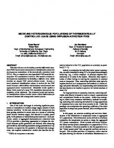
Figure 2.5: Comparison of CCCV and modified reference governor (MRG) charging. The MRG regulates ηs near its limit, thereby achieving 95% SOC in 14.9min vs. 35.5min for CCCV by allowing voltage to safely exceed 4.2V.

2.4

Numerical Results

MRG Simulations We consider the case when the constrained output variables, y, are measurable, as shown in Fig. 2.4. In practice, one needs to estimate these variables from measurements of current and voltage, as done in [30]. This chapter section analyzes performance under the hypothetical situation of output variable feedback. Prediction horizon Ts = 5 sec is used in all simulations. In the following, we apply the MRG to the scenarios described in Chapter 2.2. Figure 2.2 displays the current I(t), reference current I r (t), and side reaction overpotential ηs (L− , t) for a 10sec 3C pulse charging scenario. Note how the MRG attenuates the current to satisfy ηs > 0. Similarly, Fig. 2.3 displays the system responses for a 10sec 7C pulse discharging scenario. Again, I(t) is attenuated such that lithium is not depleted in the electrolyte. Next we demonstrate the benefits of utilizing a MRG for charging. Figure 2.5 compares the standard charging protocol, constant charging-constant voltage (CCCV), to a reference

CHAPTER 2. ENHANCED PERFORMANCE OF LI-ION BATTERIES VIA MODIFIED REFERENCE GOVERNORS & ELECTROCHEMICAL MODELS Current [C−rate]

0 −1

19

MRG, I (t) LMRG, I (t) I r (t)

−2


−3

MRG ηs (L− , t) LMRG ηs (L− , t)

0.2 0.15 0.1 0.05 0 −0.05 0

20

40

60 Time [sec]

80

100

120

Figure 2.6: Comparison of MRG and LMRG. Signals include current I(t), reference current I r (t), and side reaction overpotential ηs (L− , t) for a 10sec 3C pulse charging scenario. The LMRG does not reach the constraint, due to linearization modeling errors.

governor-based charging. In both cases, we consider a constant 1C charging current. The CCCV protocol applies 1C charging until the terminal voltage reaches a “maximum safe voltage level,” 4.2V in this case. This occurs near the 7.5 min. mark. Then CCCV regulates terminal voltage at the maximum value, 4.2V, while the current diminishes toward zero. The 4.2V limit is selected such that lithium plating does not occur due to overcharging. Indeed, the side reaction overpotential remains positive. However, this approach is conservative. Specifically, the side reaction overpotential can be regulated closer to its limit. The MRG applies 1C charging subject to the constraint ηs (L− , t) ≥ 0. In Fig. 2.5 the MRG maintains ηs ≥ 0 despite voltage exceeding 4.2V. Moreover, the cell attains 95% SOC in 14.9min using the MRG vs 35.5min for CCCV. Also note that CCCV reaches an equilibrium SOC of 96%, whereas the MRG achieves 100% SOC. Consequently, 60%-95% charging time is decreased by 58% and charge capacity is increased by 4%. Linear-MRG Simulations Next we evaluate simulations of the linear MRG (LMRG) to ascertain the trade off between computational efficiency and constraint satisfaction. Figure 2.6 compares the LMRG to the nonlinear MRG, for the 10sec 3C pulse charging scenario. In the LMRG, ηs (L− , t) does not reach the constraint, due to linearization modeling errors. This produces a conservative response that is within the constraint. The opposite is portrayed in Fig. 2.7, for the 10sec 7C pulse discharging scenario, where ce (0+ , t) violates the constraint over several time pe-


20

Electrolyte Concentraiton [kmol/m3]

Current [C−rate]

8 6 4 MRG, I (t) LMRG, I (t) I r (t)

2 0 1

MRG ce (0+ , t) LMRG ce (0+ , t)

0.8 0.6 0.4 0.2 0 0

20

40

60 Time [sec]

80

100

120

Figure 2.7: Comparison of MRG and LMRG. Signals include current I(t), reference current I r (t), and electrolyte concentration ce (0+ , t) for a 10sec 7C pulse discharging scenario. The LMRG violates the constraint, due to linearization modeling errors.

riods. One might interpret the constraint over/undershoot as follows. All the constraints can be categorized into “soft constraints” (small violations are allowable but undesirable, e.g. SEI film growth) and “hard constraints” (small violations are not allowable, e.g. electrolyte depletion). For hard constraints, the limits can be selected more conservatively to avoid overshoots. Nonetheless, the constraint violation magnitude is relatively small and the LMRG would be effective at mitigating degradation and prolonging battery life. The critical advantage of the LMRG, however, is the increased computational efficiency. That is, the LMRG computes β via the explicit expressions (2.33)-(2.37), whereas the nonlinear MRG requires nonlinear simulations and optimization. We consider the CPU time for each MRG as one measure of computational efficiency. The data provided in Table 2.1 indicates that the linear MRG reduces CPU time by over four-fold on a 2.9 GHz dual-core laptop with 16GB of RAM. Further improvements are possible via code optimization. Table 2.1: CPU Time per Simulated Time for Nonlinear and Linear MRGs. Scenario 10sec 3C charging 10sec 7C discharging

MRG 1.48 sec/sec (100%) 2.16 sec/sec (100%)

Linear MRG 0.34 sec/sec (23%) 0.39 sec/sec (18%)

Current [C−rate]

10

I r (t) I(t)

5 0

0.2 0.1

3.5 3

First voltage regulation

ηs (L−, t)

0 −0.1

V (t)

4

21

0.3

ce (0+, t)

3

Electr conc. [kmol/m3]

Voltage [V]

−5

Side Rxn Overpot. [V]


ce (0−, t) 2 1

2.5 0 1

0.8

θ(L− , t)

0.4

θ

SOC

θ(0− , t)

SOC (t)

0.6

0.5

0.2 0

320

1

310 300

θ

Temperature [K]

0

290

T(t)

0.8 θ(0+ , t)

0.6

θ(L+ t)

280 0

5

10

15

20

25

0.4

0

5

10

Time [min]

15

20

25

Time [min]

Figure 2.8: US06x3 1.4I VO: Left: Reference Current I r (t) and Current I(t), Voltage V (t), State of Charge SOC(t), Temperature T (t). Right: Side Reaction Overpotential ηs (L− , t), Electrolyte Concentration ce (0+ , t), ce (0− , t), Surface Concentrations θ(0− , t), θ(L− , t), θ(0+ , t), θ(L+ , t).

Remark 2 (Current Limits & Power Capacity) The LMRG also provides real-time estimates of the max/min safe current and power capacity. The limiting current is given by Ilim (t) = I r (t) · min {Hi | i = 1, 2, ..., Nc } ,

(2.38)

and the corresponding instantaneous power capacity is Pcap (t) = Ilim (t)V (t).

(2.39)

These variables are useful for feedback to higher-level supervisory control systems [17,18,30].

Comparative Analysis We evaluate the operational, power and energy capacity benefits of the MRG versus an industry standard Voltage-Only (VO) controller on electric vehicle-like charge/discharge cycles. For comparison purposes, we choose operational voltage limits of 2.8V and 3.9V for the VO controller. Various automotive-relevant charge/discharge cycles cases were tested. To explore


β

5

Side Rxn Overpot. [V]

Voltage [V]

0.5

0 −5 4 3.5 3

V (t)

2.5 1 SOC (t)

0.8

SOC

1

I r (t) I(t)

β(t)

0 0.4 0.2 0

Electr conc. [kmol/m3]

Current [C−rate]

10

22

ηs (L−, t)

3

ce (0+, t)

2

ce (0−, t)

1 0 1

θ(0− , t)

0.6

θ

0.4

θ(L− , t)

0.5 0

310

1 T(t)

300

θ

Temperature [K]

0.2 320

290

First variable regulation

θ(0+ , t)

0.6

θ(L+ t)

280 0

0.8

5

10

15

Time [min]

20

25

0.4

0

5

10

15

20

25

Time [min]

Figure 2.9: US06x3 (1.4I) MRG. Left: Reference Current I r (t) and Current I(t), Voltage V (t), State of Charge SOC(t), Temperature T (t). Right: β(t), Side Reaction Overpotential ηs (L− , t), Electrolyte Concentration ce (0+ , t), ce (0− , t), Surface Concentrations θ(0− , t), θ(L− , t), θ(0+ , t), θ(L+ , t).

state constraint management, reference current was scaled by factors of ×1.0, ×1.2, ×1.4 (1.0I, 1.2I, 1.4I). The MRG constraints from (2.13) - (2.16) chosen for this analysis are the: Surface Concentrations θ(0− , t), θ(L− , t), θ(0+ , t), θ(L+ , t), Electrolyte Concentration ce (0+ , t), ce (0− , t), Temperature T (t), and Side Reaction Overpotential ηs (L− , t). The constraint regions represent critical locations where the variable is most likely to be largest and smallest, respectively, for upper and lower bounds. It is assumed that that Us = 0 for the Side Reaction Overpotential ηs (L− , t), and hence are constraining Li plating from occurring. Due to space constraints, we only provide detailed examples with three concatenated US06 drive cycles (US06x3). Figure 2.8 shows simulation results for the US06x3 profile whose current is scaled up by 40% (1.4I), applied to the VO controller. The upper voltage limit is first regulated before the 1 min mark, while the electrochemical variables are still away from their limits. One could operate the battery safely beyond this maximum voltage. Additionally, electrolyte concentration at the cathode/current collector interface ce (0+ , t) falls below its lower limit near 10 min, which induces Li plating. Figure 2.9 shows the simulation results for the US06x3 profile whose current is scaled


23

320

Temp [K]

315 310 305 300 295 320

MRG VO

Expanded operating range (a)

MRG VO

Expanded operating range (b)

MRG VO

Expanded operating range (c)

Temp [K]

315 310 305 300 295 320

Temp [K]

315 310 305 300 295

3

3.2

3.4

3.6

3.8

4

4.2

Volt [V]

Figure 2.10: Temperature vs. Voltage operating points for (a) 1.0I, (b) 1.2I, and (c) 1.4I over US06x3 cycle.

up by 40% (1.4I), applied to the MRG controller. Note that the maximum Li concentration at the cathode/separator interface θ(L+ , t) limit is first regulated around the 9 min mark, yet the voltage exceeds the VO upper voltage limit before 9 min. All other constrained electrochemical states are maintained within safe limits. This expands the operating regime, safely. Expanded Operating Regime Figure 2.10 depicts the Temperature vs. Voltage operational points for the MRG vs. VO controllers for the US06x3 1.0I, 1.2I, and 1.4I current profiles. The upper voltage limit on the VO controller becomes more constrictive as the current magnitude is scaled up. The MRG safely exceeds the VO voltage limits under all conditions, as previously noted. In

CHAPTER 2. ENHANCED PERFORMANCE OF LI-ION BATTERIES VIA MODIFIED REFERENCE GOVERNORS & ELECTROCHEMICAL MODELS 4000

Power[W]

3000

MRG (a) VO

24

1000 0

2000

−1000 18

1000

19

20

21

22

23

20

21

22

23

20

21

22

23

0 −1000 4000

Power[W]

3000

MRG (b) VO

1000 0

2000

−1000 18

1000

19

0 −1000 4000

Power[W]

3000

MRG (c) VO

1000 0

2000

−1000 18

1000

19

0 −1000 0

5

10

15

20

25

Time[min]

Figure 2.11: US06x3 power responses for (a) 1.0I, (b) 1.2I, and (c) 1.4I.

automotive applications, this ultimately means the MRG is able to recuperate more energy (i.e. from regenerate braking) than the VO controller. Increased Power Capacity Figure 2.11 exemplifies how the MRG allows increased power capacity. It provides power responses for the MRG vs. VO controller for US06x3 1.0I, 1.2I, and 1.4I current profiles. As current is increased, the VO attenuates power to respect the voltage limits, whereas the MRG allows for increased power. Figure 2.12 displays the distribution of cell power for the MRG vs. VO controller. This distribution elucidates how the MRG allows for greater charge power (negative power) than the VO controller. Table 2.2 presents the mean power (discharge and charge) benefit percentage results from using the MRG over the VO controller for the US06x3 drive cycle as well as five other


25

400 MRG VO

Frequency

300 200

Expanded operating range

100 (a) 0 400 MRG VO

Frequency

300 200


100 (b) 0 400 MRG VO

Frequency

300 200


100 (c) 0 −1000

−500

0

500

1000

1500

Power [W]

Figure 2.12: US06x3 Power Histogram for (a) 1.0I, (b) 1.2I, and (c) 1.4I.

automotive drive cycles (UDDSx2, SC04x4, LA92x2, DC1, DC2) from [25]. In the most aggressive drive cycle (US06x3) the MRG achieves 11.03% and 150.61% more discharge and charge power, respectively, over the VO controller in the 1.4I case. Across all six simulated drive cycles, the MRG achieves average increases in discharge and charge power of 4.92% and 57.15%, with a standard deviation of 4.02% and 43.19%, respectively, in the 1.4I case. Increased Energy Capacity Table 2.3 presents the net energy benefits for six drive cycles (US06x3, UDDSx2, SC04x4, LA92x2, DC1, DC2). In the most aggressive drive cycle (US06x3) the MRG achieves a 22.99% net energy increase over the VO controller for the 1.4I case. Across all six simulated drive cycles, the MRG achieves an average net energy increase of 10.04% with a standard deviation of 6.05% in the 1.4I case.


26

Table 2.2: Mean power benefits of using MRG vs. VO. Drive Cycle DC1 DC2 LA92x2 SC04x4 UDDSx2 US06x3 Average Std. Dev.

Mode Discharge Charge Discharge Charge Discharge Charge Discharge Charge Discharge Charge Discharge Charge Discharge Charge Discharge Charge

1.0I 0.09% 6.17% 0.02% 6.50% 0.09% 16.66% 0.08% 15.71% 0.04% 6.02% 0.23% 44.56% 0.09% 15.94% 0.07% 13.56%

1.2I 0.24% 13.23% -0.21% 22.57% 1.79% 36.11% 0.18% 26.17% 0.18% 20.09% 5.60% 100.38% 1.29% 36.43% 2.03% 29.42%

1.4I 4.02% 21.21% -0.75% 40.38% 8.91% 58.07% 2.97% 39.11% 3.07% 33.49% 11.33% 150.61% 4.92% 57.15% 4.02% 43.19%

Table 2.3: Energy benefits of using MRG vs. VO. Drive Cycle DC1 DC2 LA92x2 SC04x4 UDDSx2 US06x3 Average Std. Dev.

2.5

1.0I 2.77% 1.06% 7.25% 4.29% 1.95% 15.34% 5.45% 4.84%

1.2I 5.59% 3.56% 11.95% 6.69% 5.71% 20.64% 9.02% 5.79%

1.4I 4.68% 7.64% 10.65% 7.34% 6.94% 22.99% 10.04% 6.05%

Conclusions

This chapter develops reference governor-based approaches to satisfying electrochemical state constraints in batteries. As a consequence, it enables one to enhance power capacity, en-


27

ergy capacity, and charging speed by eliminating the conservatism imposed by traditional operating constraints (e.g. voltage limits). The key ingredients to this approach are the following. First, we utilize a first principles electrochemical model to predict and constrain the evolution of physical degradation mechanisms. Second, a nonlinear modified reference governor (MRG) algorithm is developed assuming measurements of the constrained variables. Third, a linearized MRG is developed, which replaces simulations with an explicit function evaluation at the expense of possible constraint dissatisfaction or conservatism. A suite of simulations were executed to quantify the potential performance gains of MRGs over voltage-only regulators. We found 60%-95% charge times can be reduced by 58%, charge power can be increased by 57.15% on average, and energy can be increased by 10.04% on average, for the considered case studies.

28

Chapter 3 Sensitivity-Based Interval PDE Observers for Lithium-Ion Battery SOC Estimation 3.1

Introduction

This chapter develops sensitivity-based interval partial differential equation (PDE) observers for state-of-charge (SOC) estimation in batteries, using an electrochemical-based model with bounded uncertain parameters. The goal is to generate an interval estimate of battery SOC that mathematically relates parametric uncertainty to estimation uncertainty. Batteries are ubiquitous in applications ranging from smart phones to electrified transportation. In telecommunications, there are currently about 7.4 billion active mobile subscriptions around the globe [10]. In electrified transportation, the Electric Vehicles Initiative (EVI), a multi-government initiative to accelerate the adoption of electric vehicles (EVs) worldwide aims for 20 million EVs including plug in electric vehicles (PHEVs) and fuel cell electric vehicles (FCVs) by the year 2020 [11]. The pressing needs of battery technologies are apparent, based on cost and energy targets. Despite recent performance and cost innovations, additional improvements are necessary to reach the desired targets [11]. These facts provide overwhelming motivation for accurate and robust SOC estimation to maximize battery performance and lifetime. To this end, electrochemical models [7] have attracted significant attention from battery controls researchers, due to their potential for high accuracy predictions. The parameters of these models, however, are often characterized by a bounded interval of uncertainty. In this chapter, we seek to generate interval state estimates of lithium-ion concentration, given a simple PDE electrochemical model, measurements of current and voltage, and bounds on parameter values. Mathematically, we abstract this problem as an interval PDE observer design task, based upon sensitivity equations. The two relevant bodies of literature include electrochemical model-based SOC estimation and interval observers.

CHAPTER 3. SENSITIVITY-BASED INTERVAL PDE OBSERVERS FOR LITHIUM-ION BATTERY SOC ESTIMATION

29

Electrochemical battery models capture the spatio-temporal dynamics of lithium ion concentration, electrode potential, and Butler-Volmer kinetics. Most models in the battery controls literature have been derived from the Doyle-Fuller-Newman model [6], which includes PDEs, ODEs in space, ODEs in time, and nonlinear algebraic equations. This system of equations is generally too complex for state observer design. Consequently, researchers have combined various model reduction and estimation techniques to perform SOC estimation. These include residue grouping/Kalman filters [18], electrode averaging/extended Kalman filters [31], output error injection [32], and adaptive PDE observers [30]. The underlying electrochemical models, however, are characterized by parametric uncertainty [33]. The sensitivity of state estimates to parametric uncertainty has not been addressed in the literature. Parallel to battery SOC estimation is the theory of interval observers. In state estimation and filtering schemes, process and measurement noises are often assumed to be Gaussian. For example, the venerable Kalman filter assumes zero mean Gaussian process and measurement noise, rendering a Gaussian distribution for the state estimate [34]. That is, the Kalman filter maps additive stochastic process/measurement noise to a Gaussian distribution on the state estimate. In contrast, interval or bounding observers assume process and measurement disturbances are unknown but bounded [35, 36]. These algorithms have been studied in the context of wastewater treatment [37], biochemical processes [38], robotics [39], and bioreactors [40]. We develop a similar yet different approach that assumes specified model parameters are unknown but bounded. The approach is based upon sensitivity analysis [41] and developed within the context of PDE state observers [42], yielding a new type of interval observer. This chapter connects the aforementioned bodies of literature by developing novel interval observers based upon sensitivity equations. As such, the results provide two key contributions. First, two sensitivity-based interval observers are proposed that relate parametric uncertainty to an interval state estimate, for battery SOC estimation. Second, the sensitivity equations provide a metric for ranking parameter sensitivity, as illustrated in Chapter 3.6. A parameter sweep study tests the effectiveness of the sensitivity-based interval observers. We develop these results within the context of an electrochemical PDE model of lithium-ion batteries. This chapter extends our previous work [43] with: (i) the derivation of an analytical bound interval observer, (ii) the comparison of the analytical bound interval observer and the heuristic bound interval observer (proposed in [43]), and (iii) a numerical study of the sensitivity-based interval observers for the range of uncertain parameters. This chapter is organized as follows: The single particle model and corresponding backstepping observer have been designed in [30, 44], but are provided in Chapter 3.2 and 3.3, respectively, for completeness. Chapters 3.4 and 3.5 develop the observer sensitivity equations and formulate the interval observers. Finally, Chapters 3.6 and 3.7 provide simulation results and a summary of the key contributions.

CHAPTER 3. SENSITIVITY-BASED INTERVAL PDE OBSERVERS FOR LITHIUM-ION BATTERY SOC ESTIMATION Anode

30

Cathode

Separator Solid Electrolyte

Li +

V(t) ---Single Particle Model---

I(t)

Li+ cs

-(r,t)

I(t)

cs

+(r,t)

Li+ r

r Rs-

Rs+

V(t) = h(cs-(Rs-,t), cs+(Rs+,t), I(t))

Figure 3.1: Each electrode is idealized as a single porous spherical particle. This model results from assuming the electrolyte concentration is constant in space and time [7].

3.2

Electrochemical Model Development

The sensitivity-based interval PDE observer is based upon an observer-oriented electrochemical model and backstepping observer designed in [30, 44]. For completeness and context, we summarize the model development here.

Single Particle Model We consider the simplest of electrochemical battery models, known as the “single particle model” (SPM) [45]. This model is derived from the complete Doyle-Fuller-Newman model [6] by assuming the electrolyte Li concentration is constant in space and time [7]. This approximation is reasonably valid for low C-rates (i.e. low current magnitudes). As shown in Fig. 3.1 the model consists of two diffusion PDEs in spherical coordinates governing Li concentration dynamics in the solid phase of the negative (c− s (r, t)) and positive + (cs (r, t)) electrodes. 2 ∂c− ∂c− s s (r, t) = Ds− (r, t) + ∂t r ∂r " + ∂c+ s + 2 ∂cs (r, t) = Ds (r, t) + ∂t r ∂r "

∂ 2 c− s (r, t) , 2 ∂r # ∂ 2 c+ s (r, t) , ∂r2 #

(3.1) (3.2)

CHAPTER 3. SENSITIVITY-BASED INTERVAL PDE OBSERVERS FOR LITHIUM-ION BATTERY SOC ESTIMATION ∂c− s (0, t) = 0, ∂r ∂c+ s (0, t) = 0, ∂r

I(t) ∂c− s (Rs− , t) = − − − , ∂r Ds F a AL + ∂cs + I(t) (Rs , t) = − + + + . ∂r Ds F a AL

31 (3.3) (3.4)

The Neumann boundary conditions at r = Rs+ and r = Rs− signify the flux entering the electrode is proportional to the input current I(t). The Neumann boundary conditions at r = 0 are spherical symmetry conditions and required for well-posedness. The measured terminal voltage is governed by a combination of electric overpotential, electrode thermodynamics, and Butler-Volmer kinetics. The end result is !

−I(t) RT sinh−1 V (t) = + + + α F 2a AL+ i+ 0 (css (t)) ! RT I(t) −1 − − sinh − α F 2a− AL− i− 0 (css (t)) − − +U + (c+ ss (t)) − U (css (t)) + Rf I(t),

(3.5)

where the exchange current density ij0 and solid-electrolyte surface concentration cjss are, respectively ij0 (cjss ) cjss (t)

q

= k c0e cjss (t)(cjs,max − cjss (t)), = cjs (Rsj , t), j ∈ {+, −}. j

(3.6) (3.7)

Functions U + (·) and U − (·) in (3.5) are the open circuit potentials of each electrode material, given the surface concentration. Mathematically, these are strictly monotonically decreasing functions. This fact implies the inverse of their derivatives is finite, a property that is required in Chapter section 3.2. Further details on the electrochemical principles used to derive these equations can be found in [6, 7]. The SPM parameter definitions can be found in [44]. Note that the bulk anode SOC is defined as the normalized volume sum SOC(t) =

Z Rs− 3 r 2 c− s (r, t)dr. − )3 0 c− (R s,max s

(3.8)

This model contains the property that the total number of lithium ions is conserved [32]. Mathematically, dtd (nLi ) = 0, where nLi

Z Rs+ + + sL A 4πr2 c+ =4 s (r, t)dr + )3 0 π(R s 3

+

Z Rs− − − sL A 4πr2 c− s (r, t)dr. 4 − 3 π(R ) 0 s 3

(3.9)

This property is important, as it relates the total concentration of lithium in the cathode and anode. In previous work [30,44], we have leveraged this fact to perform model reduction for the state estimation problem.


32

Observability & Model Reduction As previously demonstrated [30, 44], the SPM is not completely observable from measurements of voltage and current only. Consequently, the SPM is reduced by approximating the cathode diffusion dynamics (3.2) by its equilibrium. This renders a completely observable model. The reduced SPM has a PDE given by (3.1), boundary conditions given by (3.3), and output equation !

−I(t) RT sinh−1 V (t) = + + + − α F 2a AL i+ 0 (αcss (t) + β) ! I(t) RT −1 − − sinh − α F 2a− AL− i− 0 (css (t)) − − +U + (αc− ss (t) + β) − U (css (t)) − Rf I(t).

(3.10)

− Note that c+ ss (t) has been replaced by αcss (t) + β. This is the critical detail of the reduced + SPM. The equilibrium of the cathode states (i.e., c+ s (r, t) = css (t)) is computed from the conservation of Li property in (3.9) to produce the relationship

c+ ss (t) = −

−

where α = − s+ LL+ and β = s

h i 1 − − − n − L Ac (t) , Li s ss + + sL A

(3.11)

nLi + . + s L A

Output Function Inversion The reduced SPM contains linear dynamics and a nonlinear output function. In general, an output injection-based estimator would be nonlinear for this class of systems. However, a linear estimator is implemented in this chapter by injecting the boundary state error as in [30, 44]. This requires the boundary state to be calculated from the measured voltage as shown by the block diagram in Fig. 3.2. The output function is invertible w.r.t. the boundary state c− ss , uniformly in the input current I(t). We show this by defining h : R × R → R, such that V (t) = h(c− ss (t), I(t)). The horizontal line test can be used to show that h is a one to one function w.r.t. c− ss (t), uniformly in I(t). As a result it is possible to determine the inverse function ϕ where c− ss (t) = ϕ(V (t), I(t)).

Normalization and State Transformation Next we perform normalization and state transformation to simplify the observer structure as done in [30, 44]. First scale the radial r and time t coordinates as follows r¯ =

r , Rs−

Ds− t¯ = t. (Rs− )2

(3.12)


33

Diffusion PDE

Diffusion PDE Copy + Output Inj. Sensitivity PDEs

Interval Estimator

Figure 3.2: Block diagram of estimation scheme where the boundary state error is injected into the estimator. The use of the boundary state c− ss is determined by ϕ(V, I), which inverts the nonlinear output w.r.t. the state, uniformly in the input current. The double spatial derivative estimates cˆ− srr (r, t) along with input current I(t) and output inversion ϕ(V, I) are fed into the sensitivity PDEs. The sensitivity estimates S1 (r, t), S2 (r, t), S3 (r, t), S4 (r, t), spatial derivatives of the sensitivity estimates S1r (r, t), S2r (r, t), S3r (r, t), S4r (r, t), and the ˆ− c− concentration estimates cˆ− s are used to calculate the interval estimates ˆ s (r, t)H,A , cs (r, t)H,A . Henceforth we will drop the bars over the space and time coordinates to simplify notation. Next we perform a state transformation to eliminate the first spatial derivative in the spherical diffusion equation (3.1). Namely, let c(r, t) = rc− s (r, t).

(3.13)

This normalization and state transformation produces the following PDE with Dirichlet and Robin boundary conditions ∂ 2c ∂c (r, t) = ε 2 (r, t), ∂t ∂r c(0, t) = 0, ∂c (1, t) − c(1, t) = −qρI(t). ∂r

(3.14) (3.15) (3.16)

and nonlinear output map given by (3.10) where c+ ss = αc(1, t) + β (see (3.11)), and − − − − c− = c(1, t). The parameter ρ = R /(D F a AL ) groups electrochemical parameters ss s s


34

together. The parameters ε and q are nominally equal to one. Respectively, they represent uncertainty in the diffusion and boundary input coefficients. This uncertainty could arise from concentration-dependent diffusivity and unequal particle sizes. In the following chapter sections, we derive interval observers that map uncertainty in these parameters to bounds on the state estimates.

3.3

Backstepping PDE Observer Design

The sensitivity-based interval PDE observers are based upon the backstepping design reported in [30, 44]. We summarize the observer design here. The state estimator structure consists of a copy of the plant (3.14)-(3.16) plus boundary state error injection, as follows ∂ 2 cˆ ∂ˆ c (r, t) = ε 2 (r, t) + p1 (r)˜ c(1, t), ∂t ∂r cˆ(0, t) = 0, ∂ˆ c (1, t) − cˆ(1, t) = −qρI(t) + p10 c˜(1, t), ∂r

(3.17) (3.18) (3.19)

where the boundary state error is given by c˜(1, t) = γϕ(V (t), I(t)) − cˆ(1, t).

(3.20)

Function ϕ(V (t), I(t)) generates the boundary state from measured voltage and current by inverting the output function, as demonstrated visually by the block diagram in Fig. 3.2, as explained in Chapter section 3.2. The parameter γ represents the uncertainty in the output inversion, and is nominally equal to one. The backstepping approach [42] is applied to design the output injection gains p1 (r) and p10 , resulting in "

#

q 2λ −λr p1 (r) = I1 (x) − I2 (x) , where x = λ(r2 − 1), 2x x 3−λ p10 = , x

(3.21) (3.22)

where λ is an observer design parameter that governs the estimation error system dynamics. Functions I1 (x) and I2 (x) are, respectively, the first and second order modified Bessel functions of the first kind. This concludes the background information for deriving the proposed sensitivity-based interval observers for electrochemical PDE models.

3.4

Observer Sensitivity Equations

The main contribution of this chapter is two interval observers based upon the aforementioned backstepping observer, and the following sensitivity equations. Consider the param-


35

eterized PDE backstepping SPM observer ∂ˆ c ∂ 2 cˆ (r, t) = ε 2 (r, t) + p1 (r) [γϕ(V (t), I(t)) − cˆ(1, t)] , ∂t ∂r cˆ(r, t0 ) = δˆ c0 (r), cˆ(0, t) = 0, ∂ˆ c (1, t) − cˆ(1, t) = −qρI(t) + p10 [γϕ(V (t), I(t)) − cˆ(1, t)] , ∂r

(3.23)

(3.24) (3.25) (3.26)

where θ = [ε, q, γ, δ]T represents the uncertain parameters, whose values are nominally given by θ0 = [ε0 , q0 , γ0 , δ0 ]T = [1, 1, 1, 1]T . The parameter δ represents uncertainty in the initial condition of the observer. Suppose the nominal observer has a unique solution denoted cˆ(r, t; θ0 ). We seek to study variations of this solution due to variations in θ. In the following, we derive sensitivity equations w.r.t. ε using the procedure outlined by Khalil in Chapter 3 of [41]. The remaining sensitivity equations w.r.t. q, γ, and δ follow an identical process. Let us re-write the PDE (3.23) in partial integro-differential equation (PIDE) form cˆ(r, t) = δˆ c0 (r) +

Z t t0

[εˆ crr (r, s; θ) + p1 (r)(γϕ(V (t), I(t)) − cˆ(1, s; θ))]ds,

cˆ(r, t0 ) = δˆ c0 (r), cˆ(0, t) = 0, cˆr (1, t) − cˆ(1, t) = −qρI(t) + p10 [γϕ(V (t), I(t)) − cˆ(1, t)] ,

(3.27)

(3.28) (3.29) (3.30)

where cˆrr = ∂ 2 cˆ/∂r2 . Taking partial derivatives of both sides w.r.t. ε yields Z t ∂ˆ crr ∂ˆ c ∂ˆ c (r, t) = [ε (r, s; θ) + cˆrr (r, s; θ) − p1 (r) (1, s; θ)]ds, ∂ε ∂ε ∂ε t0

∂ˆ c ∂ˆ c (r, t0 ) = (0, t) = 0, ∂ε ∂ε ∂ˆ cr ∂ˆ c ∂ˆ c (1, t) − (1, t) = −p10 , ∂ε ∂ε ∂ε

(3.31)

(3.32) (3.33)

where cˆr = ∂ˆ c/∂r, and since c0 (r) is independent of ε. We denote cˆε = ∂ˆ c/∂ε, and change the order of differentiation in the first term on the RHS of (3.31) ∂ 2 cˆε cˆε (r, t) = [ε 2 (r, s; θ) + cˆrr (r, s; θ) − p1 (r)ˆ cε (1, s; θ)]ds, ∂r t0 Z t

(3.34)


36

cˆε (r, t0 ) = cˆε (0, t) = 0,

(3.35)

∂ˆ cε (1, t) − cˆε (1, t) = −p10 cˆε (1, t). ∂r

(3.36)

Differentiating w.r.t. time, we find that cˆε (r, t) verifies the PDE ∂ ∂2 cε (r, t) = ε 2 cˆε (r, t; θ) + cˆrr (r, t; θ) − p1 (r)ˆ cε (1, t; θ), ∂t ∂r cˆε (r, t0 ) = cˆε (0, t) = 0, ∂ˆ cε (1, t) − cˆε (1, t) = −p10 cˆε (1, t). ∂r

(3.37)

(3.38) (3.39)

When θ = θ0 , then the RHS of (3.37) depends only on the nominal solution cˆ(r, t; θ0 ). Let S1 (r, t) = cˆε (r, t; θ0 ) be the sensitivity function. Then S1 (r, t) is the solution of the “Sensitivity PDE”: S1t (r, t) = ε0 S1rr (r, t; θ0 ) + cˆrr (r, t; θ0 ) − p1 (r)S1 (1, t; θ0 ),

(3.40)

S1 (r, t0 ) = S1 (0, t) = 0, S1r (1, t) − S1 (1, t) = −p10 S1 (1, t).

(3.41) (3.42)

Note that the sensitivity PDE is a linear diffusion-reaction equation in S1 (r, t) and driven by exogenous signal cˆrr (r, t; θ0 ) in (3.40). Similarly, the sensitivity equations w.r.t. q are computed as S2t (r, t) = ε0 S2rr (r, t; θ0 ) − p1 (r)S2 (1, t),

(3.43)

S2 (r, t0 ) = S2 (0, t) = 0, S2r (1, t) − S2 (1, t) = −ρI(t) − p10 S2 (1, t),

(3.44) (3.45)

where S2 (r, t) = cˆq (r, t; θ0 ). The sensitivity PDE is a linear diffusion-reaction equation in S2 (r, t) and driven by exogenous signal I(t) in (3.45). The sensitivity equations w.r.t. γ are computed as S3t (r, t) = ε0 S3rr (r, t; θ0 ) + p1 (r)ϕ(V (t), I(t)) − p1 (r)S3 (1, t),

(3.46)

S3 (r, t0 ) = S3 (0, t) = 0, S3r (1, t) − S3 (1, t) = p10 ϕ(V (t), I(t)) − p10 S3 (1, t),

(3.47) (3.48)


37

where S3 (r, t) = cˆγ (r, t; θ0 ). The sensitivity PDE is a linear diffusion-reaction equation in S3 (r, t) and driven by exogenous signal ϕ(V (t), I(t)) in (3.46) and (3.48). Lastly, the sensitivity equations w.r.t. δ are computed as S4t (r, t) = ε0 S4rr (r, t; θ0 ) − p1 (r)S4 (1, t),

(3.49)

S4 (r, t0 ) = cˆ0 (r), S4 (0, t) = 0, S4r (1, t) − S4 (1, t) = −p10 S4 (1, t),

(3.50) (3.51) (3.52)

where S4 (r, t) = cˆδ (r, t; θ0 ). The sensitivity PDE is a linear diffusion-reaction equation in S4 (r, t), and is autonomous. Note that Si (r, t), i ∈ {1, 2, 3, 4} quantify the sensitivity of the estimated states to variations in the uncertain parameter values. We exploit this property to also perform a sensitivity analysis in Section 3.6. Consequently, when θ is close to the nominal value θ0 , we can approximate the solution cˆ(r, t; θ) around the nominal solution cˆ(r, t; θ0 ) to first-order accuracy by, cˆ(r, t; θ) := cˆ(r, t; θ0 ) + S1 (r, t)(ε − ε0 ) + S2 (r, t)(q − q0 ) +S3 (r, t)(γ − γ0 ) + S4 (r, t)(δ − δ0 ) +O((θ − θ0 )T (θ − θ0 )).

3.5

(3.53)

Sensitivity-based Interval Observers

We are now positioned to formulate the interval observers based upon the sensitivity equations derived in the previous section of this chapter. Two interval observers are constructed and presented in this chapter section. First, we assume the parameters θ = [ε, q, γ, δ]T are unknown but bounded as follows ε ≤ ε ≤ ε,

q ≤ q ≤ q,

γ ≤ γ ≤ γ,

δ ≤ δ ≤ δ,

(3.54)

where the bounds ε, q, γ, δ, ε, q, γ, δ are known. The nominal state estimate cˆ(r, t; θ0 ) is generated from the PDE backstepping observer. Now we formulate two interval observer designs that trade-off provable bounds and conservatism.

Heuristic Bound Interval Observer A Heuristic bound interval observer with interval estimates ˆc(r, t)H , ˆc(r, t)H is computed as ˆc(r, t)H = min{ˆ c(r, t) ± S1 (r, t)(ε − ε0 ) ± S2 (r, t)(q − q0 ) ±S3 (r, t)(γ − γ0 ) ± S4 (r, t)(δ − δ0 )}, ˆc(r, t)H = max{ˆ c(r, t) ± S1 (r, t)(ε − ε0 ) ± S2 (r, t)(q − q0 ) ±S3 (r, t)(γ − γ0 ) ± S4 (r, t)(δ − δ0 )},

(3.55) (3.56)


38

where we consider all combinations of the + and − operators. Functions S1 (r, t), S2 (r, t), S3 (r, t), S4 (r, t) are solutions to the sensitivity PDEs (3.40)-(3.52). These interval estimates consider all possible cases where S1 (r, t), S2 (r, t), S3 (r, t), S4 (r, t) are positive or negative. This allows for the absolute min/max to be used as the interval estimates, which are then ˆ ˆ used to find the Heuristic interval estimates of bulk SOC SOC(t) H , SOC(t)H and voltage

Vˆ (t)H , Vˆ (t)H .

We coin this design as “heuristic,” since we have not proven that ˆc(r, t)H ≤ cˆ(r, t, ; θ) ≤ ˆc(r, t)H ∀ θ given by (3.54). However, the simulations in the following chapter section demonstrate this to be true for all cases we considered.

Analytical Bound Interval Observer Next we derive bounds ˆc(r, t)A , ˆc(r, t)A that satisfy ˆc(r, t)A ≤ cˆ(r, t, ; θ) ≤ ˆc(r, t)A ∀ θ,

(3.57)

given by (3.54). This Analytical bound interval observer is computed with L2 -spatial norms, the Triangle inequality, and Agmon’s inequality. Define the first order-accurate deviation of the estimate cˆ(r, t; θ) from the nominal solution cˆ(r, t; θ0 ) as ∆ˆ c(r, t) := cˆ(r, t; θ) − cˆ(r, t; θ0 ), ∆ˆ c(r, t) := S1 (r, t)(ε − ε0 ) + S2 (r, t)(q − q0 ) +S3 (r, t)(γ − γ0 ) + S4 (r, t)(δ − δ0 ).

(3.58) (3.59)

and assume the higher order terms are negligible. Taking the L2 -spatial norm of both sides yields k∆ˆ c(r, t)k = kS1 (r, t)(ε − ε0 ) + S2 (r, t)(q − q0 ) +S3 (r, t)(γ − γ0 ) + S4 (r, t)(δ − δ0 )k.

(3.60)

Since (ε − ε0 ),(q − q0 ),(γ − γ0 ),(δ − δ0 ) are scalar, applying the Triangle inequality gives k∆ˆ c(r, t)k ≤ kS1 (t)k · |ε − ε0 | + kS2 (t)k · |q − q0 | +kS3 (t)k · |γ − γ0 | + kS4 (t)k · |δ − δ0 |.

(3.61)

We define the following based on the bounds of the uncertain parameters ∆εmax = max {|ε − ε0 |, |ε − ε0 |} , n

o

∆qmax = max |q − q0 |, |q − q0 | , n

o

∆γmax = max |γ − γ0 |, |γ − γ0 | , n

o

∆δmax = max |δ − δ0 |, |δ − δ0 | .

(3.62) (3.63) (3.64) (3.65)


39

Applying these bounds, we can now define upper bounds on k∆ˆ c(t)k as k∆ˆ c(r, t)k ≤ kS1 (t)k · ∆εmax + kS2 (t)k · ∆qmax +kS3 (t)k · ∆γmax + kS4 (t)k · ∆δmax .

(3.66)

Similarly, we define upper bounds on k∆ˆ cr (r, t)k as k∆ˆ cr (r, t)k ≤ kS1r (t)k · ∆εmax + kS2r (t)k · ∆qmax +kS3r (t)k · ∆γmax + kS4r (t)k · ∆δmax .

(3.67)

This positions us to apply Agmon’s inequality, max |∆ˆ c(r, t)|2 ≤ 2k∆ˆ c(r, t)k · k∆ˆ cr (r, t)k.

r∈(0,1)

(3.68)

Consequently, we define an upper bound on |∆ˆ c(r, t)| as |∆ˆ c(t)|max := {2 [kS1 (t)k · ∆εmax + kS2 (t)k · ∆qmax +kS3 (t)k · ∆γmax + kS4 (t)k · ∆δmax ] · [kS1r (t)k · ∆εmax + kS2r (t)k · ∆qmax

(3.69)

+kS3r (t)k · ∆γmax + kS4r (t)k · ∆δmax ]}1/2 . We can now compute the Analytical bound interval estimates ˆc(r, t)A , ˆc(r, t)A as ˆc(r, t)A = cˆ(r, t) − |∆ˆ c(t)|max , ˆc(r, t)A = cˆ(r, t) + |∆ˆ c(t)|max .

(3.70) (3.71)

Note these definitions of ˆc(r, t)A , ˆc(r, t)A satisfy (3.57). These interval estimates are then ˆ ˆ used to find the Analytical interval estimates of bulk SOC SOC(t) A , SOC(t)A and voltage

Vˆ (t)A , Vˆ (t)A using (3.8) and (3.10), respectively.

3.6

Simulations

In this chapter section we present simulation examples of the interval PDE observers for various charge/discharge cycles, along with a sensitivity analysis and a parameter sweep study to test the effectiveness of the interval observers. We apply the observer to the reduced SPM, apply the sensitivity equations to the observer, whose results are then used in the interval observers. We work in the normalized (r, t) coordinates but retain the original state realization. The model parameters originate from [33] for a commercial LiFePO4 cell. Estimation gain parameter λ = −5 from (3.21)-(3.22), as in [44]. The uncertain parameters for the interval observers are set at θ = [0.9, 0.9, 0.9, 0.6]T and θ = [1.1, 1.1, 1.1, 1.4]T which represents a ±10% deviation from the nominal parameters ε0 , q0 , γ0 and a reasonable

0 (a)

−5 5

10

15 S1 (1, t) S2 (1, t) S3 (1, t) S4 (1, t)

1 0

Bulk SOC

1

(b)

0 0.6 0.4 0.2

0.5

0

Voltage

0 3.5 3.4

5

0

2

3.43 3.42 3.41 3.4 3.39

10 SOC(t) ˆ SOC(t) 4

15SOC(t) ˆ

ˆ SOC(t) H

A

3.5 4 4.5 5 5.5

V (t) Vˆ (t)

15

Vˆ (t)H

Vˆ (t)H Vˆ (t)A Vˆ (t) A

3.3 3.2 (d)

3.1 0

0.6

5

10 Time [min]

15

Figure 3.3: Pulse Charge/Discharge Cycle (a) Input current. (b) Sensitivity. (c) Bulk SOC. (d) Output Voltage.

20

30

10

0.6 0.5 0.4 0

20

40

2

30

4

0.4 0.2 0

10

10

50 S1 (1, t) S2 (1, t) S3 (1, t) S4 (1, t) (b)

(c)

5

(a)

1

0 0.8

H

ˆ SOC(t) A ˆ SOC(t)

6 4 2 0 −2 −4 0x 104 2

40

0

Bulk SOC

Sensitivity

0x 10 2

Sensitivity

4

Current [C−rate]

5

0 3.5 Voltage

Current [C−rate]


3.4

3.27 3.26 10 3.25 3.24 3.23 3.7

40

50

SOC(t) ˆ SOC(t)

ˆ SOC(t) H ˆ SOC(t) A

ˆ SOC(t) H

ˆ SOC(t) A (c)

20

3.8

30

3.9

40

50

V (t) Vˆ (t)

Vˆ (t)H Vˆ (t)A

Vˆ (t)H

Vˆ (t)A

3.3 3.2 0

(d)

10

20

30 Time [min]

40

50

Figure 3.4: UDDSx2 Charge/Discharge Cycle (a) Input current. (b) Sensitivity. (c) Bulk SOC. (d) Output Voltage.

range of physically meaningful observer initial conditions for the nominal parameter δ0 . All PDE models are implemented using the finite central difference method. The SPM plant and observer states are initialized at different values to demonstrate uncertainty in initial conditions. Zero mean normally distributed noise with a standard deviation of 2mV is added to the voltage measurement.

Charge/Discharge Cycles First, a pulse current charge/discharge cycle is applied. Figure 3.3(a) shows the applied current in terms of C-rate (normalized current against charge capacity), where positive values indicate discharge rates. Figure 3.3(b) shows the resulting sensitivities of surface concentration, where S3 has the largest time average, followed by S2 , S1 , and S4 . This indicates that the observer system is most sensitive to perturbations in γ, followed by q, then ε, and finally δ. More specifically, the observer system is most sensitive to the output


41

inversion ϕ as γ represents its uncertainty. Figure 3.3(c) shows the true and estimated bulk SOC along with the upper and lower interval (Heuristic and Analytical) estimates. We see that the estimate converges to within 1% of the the true value at t=4.13min. We also see that the Heuristic interval estimates encapsulate the true SOC within reasonable bounds after t=0.82min, while the Analytical interval estimates do so from the beginning. Figure 3.3(d) shows the plant output voltage with noise and estimated voltage along with the upper and lower interval estimates. At t=1.19min the voltage error between the estimated and true voltage with noise is less than 3mV. Note that both the Heuristic and Analytical interval estimates bound the estimated state ˆ SOC(t), even though we have only mathematically proven this property for the Analytic interval observer. The Analytical interval estimates are more conservative than the Heuristic estimates, due to the various majorizations performed in the previous chapter section. Consequently, the two observers trade-off provable bounds with conservatism. Next, an electric vehicle-like charge/discharge cycle consisting of two concatenated urban dynamometer driving schedules (UDDS) is applied. Figure 3.4(a) shows the applied current in terms of C-rate. Figure 3.4(b) shows the resulting sensitivities, where S3 has the largest time average, followed by S2 , S1 , and S4 . Note that this is the same observation as seen with the pulse current profile. Figure 3.4(c) shows the true and estimated bulk SOC along with the upper and lower interval (Heuristic and Analytical) estimates. We see that the estimate converges to within 1% of the the true value at t=4.25min. We also see that the Heuristic interval estimates encapsulate the true SOC within reasonable bounds after t=0.91min, while the Analytical interval estimates do so from the beginning. Figure 3.4(d) shows the plant output voltage with noise and estimated voltage along with the upper and lower interval estimates. At t=1.17min the voltage error between the estimated and true voltage with noise is less than 3mV. Similar to the pulsed current case, the Heuristic and Analytical interval estimates bound ˆ the estimated state SOC(t). Again, we see a trade-off between mathematically provable bounds and conservatism.

Sensitivity Analysis A set of electric vehicle-like charge/discharge cycles (US06x3, SC04x4, LA92x2, DC1, DC2) [25] are applied to further understand the effects of parameter uncertainty through sensitivity analysis on the observer system. We rank the parameters based on the integrated absolute value of each sensitivity normalized by time, Sranki

1ZT |Si (s)|ds, = T 0

(3.72)

where i ∈ [1, 2, 3, 4], and T is the total time. Figure 3.5 shows that estimated SOC is most sensitive to perturbations in γ, followed by q, ε, and finally δ. Consequently, accurate output inversion is most important for accurate SOC estimation.


42

Figure 3.5: Normalized parameter sensitivity ranking (average in blue, standard deviation in red) across various electric vehicle-like charge/discharge cycles (UDDSx2, US06x3, SC04x4, LA92x2, DC1, DC2).

Parameter Sweep We now explore if the proposal interval observers bound the family of state trajectories produces as we sweep the parameter values. The Heuristic and Analytical interval observer bounds from the pulse current charge/discharge cycle in Fig. 3.3 are evaluated by individually sweeping the uncertain parameters (ε,q,γ,δ) of the nominal observer from their lower to upper bounds. Figure 3.6-3.7, 3.8-3.9, 3.10-3.11, 3.12-3.13 shows the effectiveness of the Heuristic and Analytical interval observer bounds when generating a family of observer estimate trajectories of each uncertain parameter (ε,q,γ,δ) for SOC and V , respectively. We see that both interval observer bounds encapsulate the family of observer trajectories for all cases when ε ∈ [0.9, 1.1], q ∈ [0.9, 1.1], γ ∈ [0.9, 1.1], δ ∈ [0.6, 1.4], respectively. Note that the Heuristic interval observer bounds all the state trajectories for the cases considered here, although this has not been proven analytically. If one desires provable bounds, then the Analytical interval observer can be used in exchange for added conservatism. Additionally, these results verify the sensitivity analysis findings (γ having the largest effect on observer estimates) in the previous section. This is due to the fact that uncertainty in the output inversion (via uncertain parameter γ) will result in uncertainty in the observer estimates. Finally, these results also demonstrate that the observer is robust to the other uncertainties presented in this chapter, such as measurement noise and the first-order approximation in (3.53).

CHAPTER 3. SENSITIVITY-BASED INTERVAL PDE OBSERVERS FOR LITHIUM-ION BATTERY SOC ESTIMATION 0.65

SOC(t) ˆ SOC(t) −10%

0.6

ˆ SOC(t) −5% ˆ SOC(t)

3.7

0.55

ˆ SOC(t) +5% ˆ SOC(t) +10% ˆ SOC(t) H

3.6

1

0.45

0.8

5.25

5.3

5.35

5.4

0.6

ˆ SOC(t) H ˆ SOC(t) A ˆ SOC(t)

V (t) Vˆ (t)−10%

3.42

Vˆ (t)−5% Vˆ (t)

3.415 3.41

Vˆ (t)+5% Vˆ (t)+10%

3.405 3.5 Voltage

Bulk SOC

0.5

43

3.4 4.9

4.95

5

5.05

3.4

Vˆ (t)H Vˆ (t) H

Vˆ (t)A Vˆ (t) A

A

3.3

0.4 0.2

3.2

0 5

Time [min]10

15

0

Figure 3.6: Pulse Charge/Discharge Cycle SOC Trajectories for ε = {0.9, 0.95, 1.0, 1.05, 1.1}.


0.45

0.4

Bulk SOC

0.35 1 8.98

9

9.02

3.7

ˆ SOC(t) +5% ˆ SOC(t) +10%

3.6

ˆ SOC(t) H ˆ SOC(t)

3.5

0.6

ˆ SOC(t) A ˆ SOC(t)

Time [min]10

15

V (t) Vˆ (t)−10% Vˆ (t)−5%

3.42


H

0.8

5

Figure 3.7: Pulse Charge/Discharge Cycle Voltage Trajectories for ε = {0.9, 0.95, 1.0, 1.05, 1.1}.

3.415

Vˆ (t) Vˆ (t)+5% Vˆ (t)+10%

3.41 3.405

Voltage

0

4.95

5

5.05

Vˆ (t)H Vˆ (t) H

Vˆ (t) Vˆ (t)

3.4

A

A

3.3

0.4 0.2

3.2

0 0

5

Time [min]10

15

Figure 3.8: Pulse Charge/Discharge Cycle SOC Trajectories for q = {0.9, 0.95, 1.0, 1.05, 1.1}.

0

5

Time [min]10

15

Figure 3.9: Pulse Charge/Discharge Cycle Voltage Trajectories for q = {0.9, 0.95, 1.0, 1.05, 1.1}.


0.5

Bulk SOC

0.45 0.4

0.8

10

12

14

16

18

0.6


3.7


3.6

ˆ SOC(t) H ˆ SOC(t) A ˆ SOC(t)

V (t) Vˆ (t)−10%

3.315

Vˆ (t)−5% Vˆ (t)

3.31

3.5 Voltage

0.55

1

3.32


0.6

Vˆ (t)+5% Vˆ (t)+10%

3.305 3.3 13

44

13.5

14

14.5

15

Vˆ (t)H Vˆ (t) H

Vˆ (t)A Vˆ (t)

3.4

A

A

3.3

0.4 0.2

3.2

0 5

Time [min]10

Figure 3.10: Pulse Charge/Discharge Cycle SOC Trajectories for γ = {0.9, 0.95, 1.0, 1.05, 1.1}.

0.4

Bulk SOC

0.2 1 0

1

2

3

Time [min]10

15

3.35

V (t) Vˆ (t)−40%


3.7

3.3

Vˆ (t)−10% Vˆ (t)


3.6

3.25

Vˆ (t)+10% Vˆ (t)+40%

3.5

3.2

ˆ SOC(t) H ˆ SOC(t) A

0

0.5

1

1.5

Vˆ (t)H Vˆ (t) H

Vˆ (t)A Vˆ (t)

3.4

ˆ SOC(t) A

0.6

A

3.3

0.4 0.2 0 0

5

Figure 3.11: Pulse Charge/Discharge Cycle Voltage Trajectories for γ = {0.9, 0.95, 1.0, 1.05, 1.1}.


0.6

0.8

0

15

Voltage

0

3.2 5

Time [min]10

15

Figure 3.12: Pulse Charge/Discharge Cycle SOC Trajectories for δ = {0.6, 0.9, 1.0, 1.1, 1.4}.

0

5

Time [min]10

15

Figure 3.13: Pulse Charge/Discharge Cycle Voltage Trajectories for δ = {0.6, 0.9, 1.0, 1.1, 1.4}.


3.7

45

Conclusions

This chapter examines the sensitivity of a previously developed backstepping PDE estimator [30, 44] to perturbations in the nominal uncertain parameters. It then combines the resulting sensitivities with the observer estimates to generate upper and lower interval estimates, for a given deviation in the nominal uncertain parameters. The sensitivity results are also used to rank parameter sensitivity to understand which parameters have the greatest effect on the observer estimates. This is important for prioritizing which parameters to identify in a system identification process. The two proposed interval estimation algorithms compromise analytically provable bounds with tightness. We explore this trade off in simulation, and demonstrate the effectiveness via a parameter sweep analysis. Ultimately, the interval estimates can be integrated into a feedback control application to ensure robustness to parameter uncertainty.

46

Chapter 4 Optimal Charging of Li-Ion Batteries via a Single Particle Model with Electrolyte and Thermal Dynamics 4.1

Introduction

This chapter develops an approach to solve for optimal charge control schemes using an electrochemical based model with thermal dynamics. The goal is to systematically obtain optimal charge schemes that result in the lowest charge times, while understanding their nature to gain an insight on battery design optimization for fast charging. Batteries are widely utilized in mobile handsets, electric vehicles (EVs), and power grid energy storage [30, 46]. They are an enabling technology for diversifying and securing our future energy supplies. In contrast to simple and rapid refueling of gasoline or diesel, battery recharge requires meticulous control and management, owing to complex electrochemical reactions, immeasurable internal states, and serious safety concerns [47]. Fast charging is a thriving area of research, as it increases the practicality and consumer acceptance of batterypowered devices (e.g., EVs). Nevertheless, it can also impair battery longevity depending on the charging method used, particularly due to heating. It is thus crucial to systematically study the effects of electrochemical and thermal states on charging time, which is the focus of this chapter. The traditional charging protocol for Li-ion batteries is constant-current/constant-voltage (CC-CV) [23]. In the CC stage, the charging current is constant until a pre-specified voltage threshold is reached, and in the CV stage the voltage threshold is maintained until the current relaxes below a pre-specified threshold value. This technique is simple and easily implemented. The current rate and voltage threshold are, however, almost universally selected in an ad-hoc manner. In the literature, various methods have been proposed to reduce charge times, such as multi-stage CC (high CC followed by low CC) plus CV (CC-CC-CV) [48], boost charging

CHAPTER 4. OPTIMAL CHARGING OF LI-ION BATTERIES VIA A SINGLE PARTICLE MODEL WITH ELECTROLYTE AND THERMAL DYNAMICS

47

(CV-CC-CV) [49], constant power-constant voltage (CP-CV) [24], fuzzy logic [50,51], neural networks [52], grey system theory [53], and ant colony system algorithm [54]. Alternative protocols were reported to prolong the battery lifetime as well, such as MCC-CV (low CC followed by high CC plus CV) [24] and CC-CV with negative pulse (CC-CV-NP) [55]. This literature provides enormous insight on rapid charging, but all the protocols are – at some level – heuristic. That is, they employ basic knowledge, empirical observations, and experience of the battery’s electrical properties to devise a charging strategy. Their implementation and performance are subject to cumbersome meta-parameter tuning. Furthermore, there are no mathematical guarantees for fast charge optimality, nor constraint satisfaction. Recently, some researchers have given first insights into model-based optimal charge control [56–61]. A significant challenge for model-based charge control is numerically solving a multi-state nonlinear calculus of variations optimal control problem. These previous studies side-step this difficulty using linear-quadratic formulations [56], state independent electrical parameters [57], piecewise constant time discretization [58], linear input-output models [59], a one-step model predictive control formulation [60], or a reference governor formulation [61]. To directly face the nonlinear variational calculus problem, orthogonal collocation enabled pseudo-spectral methods were employed in [62] to optimize charging time and efficiency of lithium-ion batteries. This work was extended in [63] to consider aging and coupled electrical-thermal dynamics via equivalent circuit type models. However, all of the foregoing studies do not explore coupled and fully constrained electrochemical-thermal dynamics for fast charge applications. Moreover, previous model based techniques do not give insight on what parameters a battery cell designer can optimize for enabling faster charge times. This chapter pursues a different approach to developing optimal fast charging protocols using electrochemical-thermal models. Mathematically, we formulate a minimum time optimal control problem via a coupled Single Particle Model with Electrolyte and Thermal Dynamics (SPMeT). In the coupled model, two PDE single particle subsystems capture both anode and cathode solid concentration dynamics, a three-PDE electrolyte subsystem captures the electrolyte concentration dynamics in three domains (anode, separator, cathode) which all feed into the nonlinear voltage output function (4.10). The nonlinear voltage output and bulk solid concentrations are then fed into the two-state thermal subsystem (4.14), whose temperature feeds back into the nonlinear voltage output and solid/electrolyte dynamics. Due to the coupled electrochemical-thermal dynamics, the optimization problem is highly nonlinear. Consequently, there are no analytic solutions and numerical solutions have been considered extremely difficult. We challenge this entrenched mindset by leveraging the Legendre-Gauss-Radau (LGR) pseudo-spectral method with adaptive multi-mesh-interval collocation. It is also worth emphasizing that incorporating a two-state temperature model in lieu of the commonly-used single lumped temperature yields more accurate predictions and safer charging protocols. This chapter extends our previous work [64] with: (i) the incorporation of temperature dependent electrochemical model parameters and a two state thermal model, (ii) an experimental validation of the electrochemical-thermal model dynamics for charging, (iii) analysis of optimal charge protocols using the validated electrochemicalthermal model, and (iv) experimental comparison and tradeoff analysis of capacity fade and


48

V(t) Anode

Cathode

Separator

Cell

Solid

Tc(t) Ts(t)

Electrolyte

Li+

Li+ cs-(r,t) Solid

I(t)

Li+ r

r Rs-

Electrolyte

I(t)

cs+(r,t)

ce(x,t)

I(t)

I(t) Li+

0-

Rs+

Li+

Li+

L- 0sepLsep L+

0+

x

𝑠𝑒𝑝

𝑉(𝑡) = ℎ(𝑐𝑠− (𝑅𝑠− , 𝑡), 𝑐𝑠+ (𝑅𝑠+ , 𝑡), 𝑐𝑒− (𝑥, 𝑡), 𝑐𝑒 (𝑥, 𝑡), 𝑐𝑒+ (𝑥, 𝑡), 𝑇𝑎𝑣𝑔 (𝑡), 𝐼(𝑡))

Figure 4.1: Each electrode is idealized as a single porous spherical particle whose dynamics evolve in the r dimension. The electrolyte concentration dynamics evolve in all regions in the x dimension. charging time for an electrochemical-thermal model based optimal charge protocol, and a traditional CC-CV charge protocol. The remainder of this chapter is structured as follows. In Chapter 4.2, the Single Particle Model with Electrolyte and Thermal Dynamics is described. In Chapter 4.3, the minimum time optimal charge control problem is formulated, and the LGR pseudo-spectral method is briefly introduced. Optimization results are discussed in Chapter 4.4, followed by experimental results in Chapter 4.5. Finally, Chapter 4.6 concludes with a summary of the key findings.

4.2

Single Particle Model with Electrolyte and Thermal Dynamics

The Single Particle Model with Electrolyte and Thermal Dynamics (SPMeT) is summarized in this section. The Single Particle Model with Electrolyte Dynamics (SPMe) used here is most similar to [65–67] and achieves a higher prediction accuracy than the Single Particle Model without electrolyte dynamics. Complete details on the derivation and model properties of the SPMe are presented in [68]. The Thermal Model from [8, 9] is coupled to the SPMe to form the SPMeT (see Fig. 4.1).

CHAPTER 4. OPTIMAL CHARGING OF LI-ION BATTERIES VIA A SINGLE PARTICLE MODEL WITH ELECTROLYTE AND THERMAL DYNAMICS + (𝑡) 𝑐𝑠𝑠

𝑐𝑠+ (𝑟, 𝑡) 𝑐𝑠− (𝑟, 𝑡)

𝑐𝑠+ (𝑟, 𝑡)

Cathode Bulk

𝑐𝑠− (𝑟, 𝑡) − (𝑡) 𝑐𝑠𝑠

Anode Bulk

49

𝑐𝑠+ (𝑡) 𝑐𝑠− (𝑡)

𝐼(𝑡) 𝑐𝑒+ (𝑥, 𝑡) 𝑠𝑒𝑝 𝑐𝑒 (𝑥, 𝑡)

𝑐𝑒− (𝑥, 𝑡)

𝑐𝑒+ (𝑥, 𝑡)

Output

𝑉(𝑡)

𝑠𝑒𝑝

𝑐𝑒 (𝑥, 𝑡) 𝑐𝑒− (𝑥, 𝑡)

Temperature

𝑇𝑐 (𝑡) 𝑇𝑠 (𝑡) 𝑇𝑎𝑣𝑔 (𝑡)

− Figure 4.2: Block diagram of SPMeT. Note that the c+ s , cs , ce subsystems are independent of one another. However, all subsystems are coupled through temperature since it feeds back − into the nonlinear voltage output and c+ s , cs , ce subsystems.

SPMeT Model The SPMeT model consists of: (i) two linear spherical diffusion PDEs modeling each electrode’s solid concentration dynamics, (ii) a quasilinear diffusion equation (across three domains) modeling the electrolyte concentration dynamics, (iii) a nonlinear output function mapping boundary values of solid concentration, electrolyte concentration, and current to terminal voltage, and (iv) two ODEs modeling the core and surface temperature of the cell. The average temperature then feeds back into the nonlinear output function, and the solid and electrolyte dynamics (see Fig. 4.2). We now introduce the SPMeT equations. The solid diffusion equations (4.1) with boundary conditions (4.2) are ± ∂c± 1 ∂ s ± 2 ∂cs (r, t) = 2 Ds (Tavg )r (r, t) , ∂t r ∂r ∂r ∂c± ∂c± 1 s s (0, t) = 0, (Rs± , t) = ∓ ± I(t). ∂r ∂r Ds (Tavg )F a± AL±

"

#

(4.1) (4.2)

The Neumann boundary conditions at r = Rs± signify the flux entering the electrode is proportional to the input current I(t) (positive for charge). The Neumann boundary conditions at r = 0 are spherical symmetry conditions and required for well-posedness. Next, the


50

electrolyte diffusion equations (4.3)-(4.5) with boundary conditions (4.6)-(4.9) are ∂c− e ε− (x, t) e

∂ ∂c− (1 − t0c ) e = Deef f (c− , T ) (x, t) − I(t), avg e ∂t ∂x ∂x F AL− " # sep ∂csep ∂ e ef f sep sep ∂ce (x, t) = De (ce , Tavg ) (x, t) , εe ∂t ∂x ∂x " # + ∂ ∂c+ (1 − t0c ) e + ∂ce ef f + εe (x, t) = De (ce , Tavg ) (x, t) + I(t), ∂t ∂x ∂x F AL+ "

#

∂c− ∂c+ e (0− , t) = e (0+ , t) = 0, ∂x ∂x − ∂csep ∂c e − ef f sep ef f − (L , t) = De (0 , Tavg ) e (0sep , t), De (L , Tavg ) ∂x ∂x + sep ∂c ∂c Deef f (Lsep , Tavg ) e (Lsep , t) = Deef f (L+ , Tavg ) e (L+ , t), ∂x ∂x ce (L− , t) = ce (0sep , t), ce (Lsep , t) = ce (L+ , t).

(4.3) (4.4) (4.5)

(4.6) (4.7) (4.8) (4.9)

The nonlinear output function for terminal voltage is governed by a combination of electric overpotential, electrode thermodynamics, Butler-Volmer kinetics, and electrolyte potential as !

RTavg (t) I(t) V (t) = sinh−1 + αF 2a AL+¯i+ 0 (t) ! RTavg (t) −I(t) −1 − sinh αF 2a− AL−¯i− 0 (t) − − + U + (c+ ss (t)) − U (css (t))

Rf+ Rf− Rce (Tavg (t)) + + ++ − −+ I(t) a AL a AL A ! L+ + 2Lsep + L− + I(t) 2Aκef f (Tavg ) !

h

i

+ kconc (t) ln ce (0+ , t) − ln ce (0− , t) ,

(4.10)

± ± where c± ss (t) = cs (Rs , t) is the surface concentration in the solid, kconc = ± and ¯i0 (t) is the spatially averaged exchange current density

h

i αc h

± ± i± 0 (t) = k (Tavg ) css (t)

2RTavg (t) (1−t0c )k¯f (t), F

iαa

± ± c± e (x, t) cs,max − css (t)

.

(4.11)

The temperature dependent electrochemical parameters follow an Arrhenius law EaP P (Tavg ) = Pref exp R

1 Tref

−

1 Tavg

!!

.

(4.12)


51

The core and surface temperature dynamics of the cylindrical cell are governed by dTc (t) Ts (t) − Tc (t) Q(t) = + , dt Rc Cc Cc dTs (t) Tf (t) − Ts (t) Ts (t) − Tc (t) = − dt Ru Cs R c Cs

(4.13) (4.14)

− − where Q(t) = I(t)|V (t) − (U + (¯ c+ cs (t)))| is the heat generation including joule s (t)) − U (¯ heating and energy dissipated by electrode over-potentials and c¯± s (t) is the bulk concentration in the anode/cathode ± 3 Z Rs 2 ± ± (4.15) r cs (r, t)dr. c¯s (t) = (Rs± )3 0 The heat conduction resistance, convection resistance, core heat capacity, and surface heat capacity are represented by Rc , Ru , Cc , and Cs , respectively. The two states are the core Tc and surface Ts temperatures. We assume that the coolant flow rate is constant (which translates to a constant Ru ), and the ambient temperature Tf is nearly constant as done in [8, 9]. The average cell temperature is

Tavg (t) =

Tc (t) + Ts (t) , 2

(4.16)

which is approximately equal to the radial average temperature [69] for the cell considered in this study. The thermal parameters have been identified in previous work [8, 9]. We determine Ru using our experimental setup as described in Chapter 4.5. We define the cell SOC from the bulk anode SOC and the stoichiometric difference in the anode as c¯− s (t) . (4.17) SOC(t) = − cs,max |x100% − x0% | This summarizes the SPMeT which maintains accuracy at higher C-rates than that of an SPM with thermal dynamics alone [68]. The model parameters used in this study originate from [9, 22, 65, 70–72] and correspond to a lithium iron phosphate cathode / graphite anode chemistry A123 26650 2.3Ah cell. We determine some parameters based on our experimental setup and validate the effectiveness of the electrochemical-thermal model for various charging cases in Chapter 4.5. Comparison to existing SPMe Models The models in [65–67] are most similar to the SPMe presented here with a few critical differences. In [65], bulk solid concentration is used in the voltage output function instead of the surface concentration we use here (see (26) in [65]). In the case of [66], volume averaging is performed in the electrolyte phase which partially obscures electrolyte polarization. In [67], the authors use an approximation of the solid state diffusion equation instead of retaining the PDE version we use in (4.1)-(4.2) (see Section 2 of [67]). Moreover, we include a temperature submodel, as does [65].


4.3

52

Optimal Charge Control Formulation

Next we formulate a minimum-time/safe optimal charge control problem. The objective function J is given by Z min

I(t),x(t),tf

tf

1 · dt,

(4.18)

t0

where (tf − t0 ) is the charge time to reach a desired target SOC (SOCf ). The optimization variables are the input current I(t) and final time tf , with state variables x(t) = − + sep − T [c+ s (r, t), cs (r, t), ce (x, t), ce (x, t), ce (x, t), Tc (t), Ts (t)] . The constraints include the model dynamics and boundary conditions (4.1) - (4.9), input, state, event, and time constraints below: Imin ≤ I(t) ≤ Imax , c± (r, t) ± ± ≤ θmax , θmin ≤ s cs,max ce,min ≤ cle (x, t) ≤ ce,max , l ∈ {−, sep, +} Tmin ≤ Tm (t) ≤ Tmax , m ∈ {c, s} t0 ≤ tf ≤ tmax , ± c± s (r, t0 ) = cs,0 ,

cle (x, t0 ) = cle,0 ,

l ∈ {−, sep, +}

SOC(tf ) = SOCf , SOC(t0 ) = SOC0 , Tm (t0 ) = T0 , m ∈ {c, s}.

(4.19) (4.20) (4.21) (4.22) (4.23) (4.24) (4.25) (4.26)

Constraints (4.20) - (4.21) protect the solid active material and electrolyte from lithium depletion/oversaturation. Constraint (4.22) protects against excessively cold or hot temperatures that accelerate cell aging. The PDE system (4.1)-(4.9) is discretized in space using a second-order accurate finite central difference method that conserves lithium [73], resulting in a nonlinear differential algebraic equation system. Due to this complex mathematical structure, it is difficult to use conventional optimization techniques, e.g., dynamic programming, Pontryagin’s minimum principle, and indirect methods, due to intractable computational burden or accuracy. Instead, we pursue pseudo-spectral methods to transcribe this infinite-dimensional optimal control problem into a finite-dimensional optimization problem with algebraic constraints at the discretized nodes. Then, the optimization variables at such nodes are solved by off-theshelf nonlinear programming (NLP) solvers, like SNOPT or IPOPT [74]. Note that convexity is not guaranteed, and therefore these solvers yield locally optimal solutions. Pseudo-spectral methods are an effective tool for complex nonlinear optimal control problems and have been extensively applied to real-world optimization problems in engineering, including aerospace and autonomous flight systems [75], road vehicle systems [76], energy storage [62, 63], etc. There are a myriad of approaches for discretizing integral and differential equations, leading to a spectrum of pseudo-spectral variants. In this study, we use the Legendre-Gauss-Radau (LGR) pseudo-spectral method with adaptive multi-mesh-interval collocation, featured by

SOC

0

0

0.5

1

1.5

3.8 3.7 3.6 3.5

2.5

3

V (t)8.5C

1 0.8 0.6 0.4 0.2 0 325

0.5

1

1.5

2

0.5

1

1.5

3

2

2.5

3

Ts (t)8.5C 0

0.5

1

1.5

4

3.5

2

2.5 3 Time (min)

3.5

4

5

4.5

5

4

4.5

5

Tc (t)6C

Ts (t)7.25C

0.6

θ −(t)8.5C θ −(t)7.25C θ −(t)6C

0.4 0.2 1.5

SOC(t)6C

Tc(t)7.25C

3.5

4.5

V (t)6C

SOC(t)7.25C

Tc (t)8.5C

305 295

3.5

V (t)7.25C

2.5

SOC(t)8.5C

315

285

2

0

1

2

3

4

− c− e (0 ,t)8.5C − ,t) c− (0 7.25C e − c− (0 ,t)6C e

1

0.5

0.3 0.2 0.1

5

θ +(t)8.5C θ +(t)7.25C θ +(t)6C

0.4

3

0

1

4.5

5

0

0

1

2 3 Time (min)

4

5

2

3

4

5

2.5 2 1.5

+ c+ e (0 ,t)8.5C + ce (0+ ,t)7.25C + c+ e (0 ,t)6C

1

Ts (t)6C 4

53

0.5 0.8

Normalized Surf. Conc.

I (t)6C

4

0

Temperature (K)

I (t)7.25C

Elec. Conc. (kmol/m3)

I (t)8.5C

8


12


Voltage (V) Current (C−Rate)


0.5

0

1

2 3 Time (min)

4

5

Figure 4.3: Minimum time charge results with Imax = {8.5C, 7.25C, 6C}. Left: Current I(t), Voltage V (t), State of Charge SOC(t), Temperatures Tc (t), Ts (t). Right: Surface Concen− + + trations θ− (t), θ+ (t), Electrolyte Concentrations c− e (0 , t), ce (0 , t). the general purpose optimal control software (GPOPS-II) [74]. This software incorporates an orthogonal collocation method to generate the LGR points. Rather than a traditional fixed global mesh, an adaptive mesh refinement algorithm is employed to iteratively adjust the number of mesh intervals, the width of each interval, and the polynomial degree (the number of LGR points). Theoretical and algorithmic properties of this method are elaborated in [77, 78] and in the Appendix.

4.4

Results and Discussion

This section presents optimization results for minimum-time charge and examines solution sensitivity to perturbations in model parameters.

Minimum Time Charge The optimal charge trajectories are shown in Fig. 4.3 for Imax = {8.5C, 7.25C, 6C}. It takes 4.48min to achieve a target SOC of 75% (SOCf = 0.75) from an initial SOC of 25% (SOC0 = 0.25) when Imax = 8.5C. The charge process follows a constant-current/constantelectrolyte-concentration/constant-surface-concentration (CC-CCe-CCss) protocol. To minimize charging time, the maximum C-rate is applied initially, causing the minimum electrolyte concentration constraint to become active at the anode current collector. The surface concentration at the anode increases until it reaches its maximum value, which becomes the dominant inequality constraint. A similar behavior is observed when Imax = 7.25C, with a

0.5

0.5

1

1.5

2

2.5

3

3.5

4

V (t)6C

4.5

5

V (t)6C,CCCV

3.6 3.5 0 1 0.8 0.6 0.4 0.2 0 325

0.5

1

1.5

2

2.5

3

3.5

SOC(t)6C

0.5

1

1.5

2

315

2.5

3

4

4.5

3.5

4

4.5

5

Tc(t)6C

Tc (t)6C,CCCV

Ts (t)6C

Ts (t)6C,CCCV

305 295 285 0

0.5

1

1.5

2

2.5 3 Time (min)

3.5

4

4.5

0.6 0.4

5

θ −(t)6C θ −(t)6C,CCCV

0.2

5 1.2

SOC(t)6C,CCCV


0 0 3.8 3.7

I (t)6C,CCCV

I(t)6C

2

0.8

0

1

2

3

4

1 0.8 0.6 0.4 0.2

0

1

2 3 Time (min)

4

5

54

θ +(t)6C θ +(t)6C,CCCV

0.4 0.3 0.2 0.1 0

5

− c− e (0 ,t)6C − ,t) c− (0 6C,CCCV e

3 Elec. Conc. (kmol/m3)

4


6


Temperature (K)

SOC

Voltage (V)

Current (C−Rate)


0

1

2

3

4

5

2.5 2 1.5 + c+ e (0 ,t)6C + ,t) c+ (0 6C,CCCV e

1 0.5

0

1

2 3 Time (min)

4

5

Figure 4.4: Optimized charge vs. CC-CV charge trajectories with Imax = 6C. Left: Current I(t), Voltage V (t), State of Charge SOC(t), Temperatures Tc (t), Ts (t). Right: Surface − + + Concentrations θ− (t), θ+ (t), Electrolyte Concentrations c− e (0 , t), ce (0 , t). longer initial current at the maximum C-rate. It takes 4.62min to achieve the target SOC in this case, which is slightly more than the previous case. Note that once the the minimum electrolyte concentration constraint becomes active at the anode current collector, the protocol follows almost the same trajectory as the previous case. A slightly different behavior is observed when Imax = 6C, which just has 2 steps. It takes 5.20min to achieve the target SOC in this case, which is longer in time than the previous cases. This protocol follows a constant-current/constant-surface-concentration (CC-CCss) protocol. The maximum Crate is applied initially, until the maximum surface concentration at the anode constraint becomes active. Heuristically, the first two protocols where Imax = {8.5C, 7.25C} are similar in nature to the CC-CC-CV charge protocol [48] which involves an initial high constant current period, followed by a lower constant current period, and then by a constant voltage period. The last protocol where Imax = 6C is similar in nature to the well known CC-CV protocol [23]. A comparison of the optimized charge protocol vs. the well known CC-CV protocol is presented in Fig. 4.4 for Imax = 6C. We make two observations. (i) It takes the CCCV protocol 5.27min to achieve the target SOC, a 0.07min (1.37%) increase w.r.t. the optimized charge protocol at Imax = 6C. (ii) The optimized protocol allows safe excursions beyond the 3.6V upper limit in CC-CV by ensuring the electrochemical state constraints are satisfied. Although the optimized protocol is not significantly faster than the CC-CV protocol here, it allows for safe charging since the CC-CV protocol violates the surface concentration constraints at the anode and cathode chosen in this study.

4 0

0

SOC

0.5

1

1.5

2

V (t)8.5C,+2.5%

3.8

2.5

3

V (t)8.5C

3.5

4

4.5

V (t)8.5C,−2.5%

3.7 3.6

0.5 0.8 0.6 0.4

θ −(t)8.5C,+2.5% θ −(t)8.5C θ −(t)8.5C,−2.5%

0.2

3.5 0.5

1

1 SOC(t)8.5C,+2.5% 0.8 0.6 0.4 0.2 0 0.5 1 325 315

1.5

2

2.5

3

SOC(t)8.5C

1.5

2

2.5

3.5

4

4.5

SOC(t)8.5C,−2.5%

3

3.5

4

4.5

Tc(t)8.5C,+2.5%

Tc(t)8.5C

Tc (t)8.5C,−2.5%

Ts (t)8.5C,+2.5%

Ts (t)8.5C

Ts (t)8.5C,−2.5%

305 295 285

0

0.5

1

1.5

2 2.5 Time (min)

3

3.5

4

4.5

1.5

0

1

2

3

0.5

0

0

1

2 3 Time (min)

55

θ +(t)8.5C,+2.5% θ +(t)8.5C θ +(t)8.5C,−2.5%

0.4 0.3 0.2 0.1

4

− c− e (0 ,t)8.5C,+2.5% − ,t) c− (0 8.5C e − − ce (0 ,t)8.5C,−2.5%

1


8

0

Temperature (K)

I (t)8.5C,−2.5%

I(t)8.5C

0

1

2

3

4

3 Elec. Conc. (kmol/m3)

I(t)8.5C,+2.5%


12


Voltage (V) Current (C−Rate)


4

2.5 2 1.5

+ c+ e (0 ,t)8.5C,+2.5% + ce (0+ ,t)8.5C + c+ e (0 ,t)8.5C,−2.5%

1 0.5

0

1

2 3 Time (min)

4

Figure 4.5: Influence of a ±2.5% deviation in De (ce , Tavg ) on optimization results for minimum time charge with Imax = 8.5C. Left: Current I(t), Voltage V (t), State of Charge SOC(t), Temperatures Tc (t), Ts (t). Right: Surface Concentrations θ− (t), θ+ (t), Electrolyte − + + Concentrations c− e (0 , t), ce (0 , t).

Sensitivity Based Battery Design for Fast Charging Next we examine the solution sensitivity to perturbations in model parameters for fast charging. In previous results, we noted that the first electrochemical constraint to become active was the electrolyte concentration at the anode current collector when Imax = {8.5C, 7.25C}. This observation motivates exploring how alterations to the electrolyte dynamics impact minimum charge time. We also explore how changes in other model parameters affect the minimum charge time. Electrolyte Diffusivity De (ce , Tavg ) A comparison between the optimized charge protocol for a ±2.5% deviation in De (ce , Tavg ) and the solution with nominal parameters is shown in Fig. 4.5 for Imax = 8.5C. The optimized charge protocol with a +2.5% deviation requires 4.40min to achieve the target SOC. The cell with greater electrolyte diffusivity requires 0.08min (1.83%) less charge time. Consequently, increasing De (ce , Tavg ) is favorable to obtaining a faster charge time. The optimized charge protocol with a −2.5% deviation requires 4.57min to achieve the target SOC. The cell with lower electrolyte diffusivity requires 0.09min (1.87%) more charge time. Consequently, decreasing De (ce , Tavg ) is not favorable to obtaining a faster charge time. Note that the trajectories are similar to that of the unperturbed solution. The difference is seen in the electrolyte concentration dynamics which become faster or slower depending on the increase or decrease in De (ce , Tavg ), respectively.


56

Other Parameters t0c , Ds+ (Tavg ), Rs+ , Ru Similarly, we examine the impact of the transference number t0c , solid diffusivity of the cathode Ds+ (Tavg ), solid particle radius of the cathode Rs+ , and cooling convection coefficient Ru on the minimum charge time. The results are summarized in Table 4.1. Note that an increase in the transference number t0c , solid diffusivity of the cathode Ds+ (Tavg ), and cooling convection coefficient Ru is favorable to obtaining a faster charge time. However, an increase in the solid particle radius of the cathode Rs+ is not favorable to obtaining a faster charge time. An increase in the transference number t0c effectively scales down the input current to the electrolyte diffusion dynamics which translates to a higher current allowed for fast charging before the constraint is reached. Increasing the solid diffusivity of the cathode Ds+ (Tavg ) speeds up the solid diffusion dynamics, and scales down the input current at the boundary which allows for a higher current when fast charging before the constraint is reached. Furthermore, increasing the cooling convection coefficient Ru means there is less cooling of the battery which translates to higher overall temperatures that is favorable for fast charging (since the dynamics of the solid and electrolyte speed up, and overall resistance of the cell goes down). Table 4.1: Minimum Charge Times for Perturbed Solutions. Parameter t0c + Ds (Tavg ) Rs+ Ru

4.5

Chg. Time (+2.5%) 4.43min 4.48min 4.58min 4.47min

Chg. Time (-2.5%) 4.53min 4.53min 4.48min 4.49min

Experimental Results and Discussion

Various experiments were conducted to validate the electrochemical-thermal model constructed in this chapter using parameters from [9, 22, 65, 70–72] for a 2.3Ah A123 26650 LiFePO4 battery in our test facility. The cell was placed on an Arbin High Current Cylindrical Cell Holder inside of an ESPEC BTL-433 environmental chamber to regulate the ambient temperature at 25o C (298.15K). A K-type thermocouple was placed on the surface of the battery to measure Ts . First, the cell was cycled using a C/20 CC-CV test to identify open circuit voltage (and open circuit potentials) using a PEC SBT2050 cycler that controls the input current to the battery. Then a 5C CC-CV charge test was performed to identify some electrochemical-thermal parameters for our experimental setup. The resulting SPMeT optimal charge protocols with Imax = {8.5C, 7.25C, 6C} from the optimization results (using the newly determined open circuit potentials and electrochemical-thermal parameters) are then applied to the battery for validation of the output voltage and surface temperature of

Anode OCP [V]

Cathode OCP [V] Open Circuit Voltage [V]


57

4 3.5 3

(U + (θ + ) − U −(θ −))Est (U + (θ + ) − U −(θ −))Exp

2.5 2

0

0.1

0.2

0.3

3.7

0.4

0.5 0.6 Cell SOC

0.7

0.8

0.9

1

U + (θ + )

3.6 3.5 3.4

0.1

0.2

1.5

0.3 0.4 0.5 Normalized Concentration

0.6

0.7

U − (θ − )

1 0.5 0

0

0.1

0.2

0.3 0.4 0.5 Normalized Concentration

0.6

0.7

Figure 4.6: Experimental Determination of Open Circuit Potentials from Open Circuit Voltage: Estimated Open Circuit Voltage (U + (θ+ ) − (U − (θ− ))Est , Experimental Open Circuit Voltage (U + (θ+ ) − U − (θ− ))Exp , Cathode Open Circuit Potential U + (θ+ ), and Anode Open Circuit Potential U − (θ− ).

the electrochemical-thermal model. We experimentally compare the SPMeT optimal charge protocol with Imax = 6C against a 5C CC-CV charge protocol (C-rate chosen based on higher charge time) on two cells. The two cells undergo several hundred cycles to determine the changes in capacity fade and charge time.

Electrochemical-Thermal Model Validation The open circuit voltage is determined from a C/20 CC-CV cycling test (with voltage limits of 3.6V and 2.0V) by taking the average of the charge and discharge voltage curves, and is used to determine the open circuit potentials of the cathode and anode (shown in Fig. 4.6). Some electrochemical-thermal parameters were determined from a 5C CC-CV charge protocol applied to a battery at 25% SOC and 25o C (298.15K). The final conditions of the applied 5C CC-CV charge protocol are 75% SOC and 31.45o C (304.6K). The current for the SPMeT optimal charge optimization results with Imax = {8.5C, 7.25C, 6C} are then applied (open loop) to validate the voltage and surface temperature of the electrochemical-thermal model, as shown in Fig. 4.7-4.9 which achieves a Voltage RMSE of {25.9mV, 23.9mV, 16.3mV} and a Surface Temperature RMSE of {0.16K, 0.17K, 0.37K}, respectively.

Current (C−rate)

CHAPTER 4. OPTIMAL CHARGING OF LI-ION BATTERIES VIA A SINGLE PARTICLE MODEL WITH ELECTROLYTE AND THERMAL DYNAMICS 10

58

I (t)

7.5 5 2.5 0

0

0.5

1

1.5

2

2.5

3

3.5

4

Temperature (K)

Voltage (V)

3.7 3.6 3.5

V (t)S PM eT

3.4

V (t)Exp

3.3 3.2 0 320

0.5

1

1.5

2

Tc (t)S PM eT

315

2.5

3

3.5

Ts (t)SP M eT

4

Ts (t)Exp

310 305 300 295

0

0.5

1

1.5

2 2.5 Time (min)

3

3.5

4

Current (C−rate)

Figure 4.7: Experimental Validation of Electrochemical-Thermal Model via SPMeT Optimal Charge Protocol when Imax = 8.5C: Current I(t), Model Voltage V (t)SP M eT , Experimental Voltage V (t)Exp , Model Temperatures Tc (t)SP M eT , Ts (t)SP M eT , and Experimental Temperature Ts (t)Exp .

10

5 2.5 0

Voltage (V)

3.7

Temperature (K)

I (t)

7.5

0

0.5

1

1.5

2

2.5

3

3.5

4

4.5

3.6 3.5

V (t)S PM eT

3.4

V (t)Exp

3.3 3.2 0 320

0.5

1

1.5

Tc (t)S PM eT

315

2

2.5

3

3.5

Ts (t)SP M eT

4

4.5

Ts (t)Exp

310 305 300 295 0

0.5

1

1.5

2 2.5 Time (min)

3

3.5

4

4.5

Figure 4.8: Experimental Validation of Electrochemical-Thermal Model via SPMeT Optimal Charge Protocol when Imax = 7.25C: Current I(t), Model Voltage V (t)SP M eT , Experimental Voltage V (t)Exp , Model Temperatures Tc (t)SP M eT , Ts (t)SP M eT , and Experimental Temperature Ts (t)Exp .

Temperature (K)

Voltage (V)

Current (C−rate)


59

10

I (t)

7.5 5 2.5 0 0 3.7

0.5

1

1.5

2

2.5

3

3.5

4

4.5

5

3.6 3.5

V (t)S PM eT

3.4

V (t)Exp

3.3 3.2 0 320

0.5

1

1.5

2

Tc (t)S PM eT

315

2.5

3

3.5

4

Ts (t)SP M eT

4.5

5

Ts (t)Exp

310 305 300 295 0

0.5

1

1.5

2

2.5 3 Time (min)

3.5

4

4.5

5

Figure 4.9: Experimental Validation of Electrochemical-Thermal Model via SPMeT Optimal Charge Protocol when Imax = 6C: Current I(t), Model Voltage V (t)SP M eT , Experimental Voltage V (t)Exp , Model Temperatures Tc (t)SP M eT , Ts (t)SP M eT , and Experimental Temperature Ts (t)Exp .

Charge Protocol Aging Two cells were used to determine the tradeoffs between capacity fade and charge time for a fixed 1.15Ah charge throughput (using the SPMeT optimal charge protocol with Imax = 6C and 5C CC-CV charge protocols). Both cells are discharged with a 1C CC-CV protocol to the open circuit voltage corresponding to 25% SOC. The charge and discharge protocol of each cell is then repeated for hundreds of cycles. The current from the SPMeT optimal charge protocol with Imax = 6C is applied to the first battery cell (open loop). The 5C CC-CV charge protocol is applied to the second battery cell (closed loop), using the builtin controller of the battery cycler to maintain the 3.6V limit under the 5C CC-CV charge operation. That is, the same current is applied each time for the SPMeT optimal charge protocol with Imax = 6C (regardless of what voltage is measured) while the current for the CC-CV protocol is adjusted in real-time once the voltage constraint becomes active. The discharge capacity is determined using a 1C CC-CV cycling test at cycles {0, 10, 60, 110, 160, 210} and is shown (normalized against initial capacity) in the first subplot of Fig. 4.10. The normalized capacity of the SPMeT optimal charge protocol with Imax = 6C is 81.18% while that of the 5C CC-CV charge protocol is 97.67% at cycle 210. The higher capacity fade experienced by the SPMeT optimal charge protocol with Imax = 6C is expected since it is applied in a pure open loop fashion and has a faster charge time than that of the 5C CC-CV protocol. The charge time of the SPMeT optimal charge protocol with Imax = 6C stays the same each time while that of the 5C CC-CV protocol increases as shown in the bottom

60

100

Charge Time [min]

Normalized Capacity [%]

CHAPTER 4. OPTIMAL CHARGING OF LI-ION BATTERIES VIA A SINGLE PARTICLE MODEL WITH ELECTROLYTE AND THERMAL DYNAMICS 90 80 5C CCCV SPMeT Optimal Charge Imax = 6C

70 60 0

50

100 Cycle Number

150

200

50

100 Cycle Number

150

200

7 6.5 6 5.5 5

0

Figure 4.10: SPMeT Optimal Charge with Imax = 6C (Open Loop) and 5C CC-CV Charge Protocol (Closed Loop) Aging: Capacity Fade, and Charge Time.

subplot of Fig. 4.10. The charge time of the SPMeT optimal charge protocol with Imax = 6C is 5.20 minutes while that of the 5C CC-CV charge protocol is initially 6.01 minutes. The charge time of the 5C CC-CV charge protocol increases to 6.23 minutes at cycle 210. There is a clear tradeoff between degradation and charge time between the SPMeT optimal charge protocol with Imax = 6C and 5C CC-CV charge protocol. These results provide motivation and justification for closed loop control to alleviate aging that occurs with time.

4.6

Conclusions

An optimal control framework for a PDE system has been developed to explore modelbased fast-safe charging protocols. In this framework, a coupled Single Particle Model with Electrolyte and Thermal Dynamics is incorporated to account for solid and electrolyte phase concentration constraints, as well as thermal constraints. The Legendre-Gauss-Radau (LGR) pseudo-spectral method with adaptive multi-mesh-interval collocation is leveraged to solve the infinite dimensional nonlinear optimal control problem. Charge time is examined subject to both electrochemical and thermal constraints. The resulting minimum time charge regimes with varying input current limits are analyzed in detail, with the following key findings: (i) The protocol is constant-current/constant-electrolyte-concentration/constantsurface-concentration (CC-CCe-CCss) when Imax = {8.5C, 7.25C}, requiring 4.48 minutes and 4.62 minutes to charge the battery from 25% to 75% SOC, respectively. This optimized protocol is similar to the heuristic high constant current-low constant currentconstant voltage (CC-CC-CV) protocol. (ii) The protocol is constant-current/constantsurface-concentration (CC-CCss) when Imax = 6C, requiring 5.20 minutes to charge the


61

battery and is similar to the well known constant-current/constant-voltage (CC-CV) protocol. (iii) The protocol solutions yield physical insight on which battery design parameters to optimize for fast charging applications. Increasing electrolyte diffusivity coefficient De (ce ), transference number t0c , solid diffusivity of the cathode Ds+ (Tavg ) and cooling convection coefficient Ru results in faster charge time when Imax = 8.5C. However, an increase in the solid particle radius of the cathode Rs+ results in slower charge time when Imax = 8.5C. Finally, experimental validation results of the SPMeT optimal charge protocol with Imax = 6C (open loop) versus a 5C CC-CV charge protocol (closed loop) are presented with respect to capacity fade and charge time.

62

Chapter 5 Optimal Charging of Li-Ion Batteries with Coupled Electro-Thermal-Aging Dynamics 5.1

Introduction

This chapter develops an approach to solve for optimal charge control schemes using an equivalent circuit based model with thermal dynamics. The goal is to systematically obtain optimal charge schemes that result in minimum-time/health-conscious protocols, while understanding their nature to gain an insight on battery system optimization for optimal charging. Batteries are widely used in mobile handsets, electric vehicles (EVs), and electric grid energy storage [46, 79]. They are an enabling technology for diversifying and securing our future energy supplies. In contrast to simple and rapid refueling of gasoline or diesel, battery recharge requires meticulous control and management, owing to complex electrochemical reactions, immeasurable internal states, and serious safety concerns [47]. Fast charging is a thriving area of research, as it increases the practicality and consumer acceptance of batterypowered devices (e.g., EVs). Nevertheless, it can also impair battery longevity depending on the charging method used, particularly due to heating. It is thus crucial to systematically study the tradeoffs between charging time and health degradation, which is the focus of this chapter. The traditional charging protocol for Li-ion batteries is constant-current/constant-voltage (CCCV) [23]. In the CC stage, the charging current is constant until a pre-specified voltage threshold is reached; in the CV stage the voltage threshold is maintained until the current relaxes below a pre-specified threshold value. This technique is simple and easily implemented. The current rate and voltage threshold are, however, almost universally selected in an ad-hoc manner. Various methods were proposed to reduce charge times. Examples include multi-stage CC

CHAPTER 5. OPTIMAL CHARGING OF LI-ION BATTERIES WITH COUPLED ELECTRO-THERMAL-AGING DYNAMICS

63

(high CC followed by low CC) plus CV (MCC-CV) [48], fuzzy logic [50, 51], neural networks [52], grey system theory [53], and an ant colony system algorithm [54]. Alternative protocols were reported to prolong the battery lifetime as well, such as MCC-CV (low CC followed by high CC plus CV) [24] and CCCV with negative pulse (CCCV-NP) [55]. These protocols are almost always heuristic. That is, they employ basic knowledge or empirical observations of electrical properties of batteries to devise a charging strategy. Their implementation and performance are subject to cumbersome meta-parameter tuning. Furthermore, there are no mathematical guarantees for fast charge optimality or safe constraint satisfaction. Recently, some researchers have given first insights into model-based optimal charge control [56–61]. A significant challenge for model-based charge control is numerically solving a multi-state nonlinear calculus of variations optimal control problem. These previous studies side-step this difficulty using linear-quadratic formulations [56], state-independent electrical parameters [57], piecewise constant time discretization [58], linear input-output models [59], a one-step model predictive control formulation [60], or a reference governor formulation [61]. To directly face the nonlinear variational calculus problem, orthogonal collocation enabled pseudo-spectral methods were employed in [62] to optimize charging time and efficiency of lithium-ion batteries. However, all of the foregoing studies merely consider the electrical behavior of batteries, without simultaneously accounting for thermal and aging dynamics. Consequently, the optimized protocols may markedly deviate from reality, as batteries invariably work at varying thermal and aging conditions. Moreover, one cannot explore aging minimization and temperature-related safety considerations (e.g., thermal runaway). This chapter pursues a different approach to developing optimally health-conscious fastsafe charging protocols. Mathematically, we formulate a multi-objective optimal control problem via a coupled electro-thermal-aging model. In the full model, a two-state thermal subsystem captures both core and surface temperature dynamics. The core temperature feeds into parameters within the electrical and aging subsystems [9]. Due to the bi-directional coupling between subsystems, the optimization problem is highly nonlinear. Consequently, there are no analytic solutions and numerical solutions have been previously considered intractable. We challenge this entrenched mindset by leveraging the Legendre-Gauss-Radau (LGR) pseudo-spectral method with adaptive multi-mesh-interval collocation. To the best of our knowledge, it is the first multi-objective optimization framework for optimally trading off charging time and battery capacity fade, subject to both electrical and thermal limits. It is also worth highlighting that incorporating a two-state temperature model in lieu of the commonly-used single lumped temperature yields more accurate predictions and safer charging protocols. This article extends our previous work [63] with: (i) an experimental validation of the electro-thermal model dynamics for charging, (ii) analysis of optimal charge protocols using the aging model coupled to the validated electro-thermal model, and (iii) experimental comparison and tradeoff analysis of capacity fade and charging time for a balanced charge and traditional CCCV protocol. The remainder of this chapter is structured as follows. In Chapter 5.2, the coupled electro-thermal-aging model is described. In Chapter 5.3, the multi-objective optimal control problem is formulated, and the LGR pseudo-spectral method is briefly introduced. Opti-

CHAPTER 5. OPTIMAL CHARGING OF LI-ION BATTERIES WITH COUPLED ELECTRO-THERMAL-AGING DYNAMICS R1

C1 V1

Voc

R2

C2 V2

R0

64

+ Vt -

Figure 5.1: Schematic of the Electrical Model.

mization results are discussed in Chapter 5.4, followed by experimental results in Chapter 5.5. Finally, Chapter 5.6 summarizes the key findings.

5.2

Coupled Electro-Thermal-Aging Model

In this section, a coupled electro-thermal-aging model is described for cylindrical lithiumiron-phosphate batteries (A123 ANR26650M1). It consists of a second-order equivalent circuit model for emulating voltage behavior, a two-state thermal model for predicting the core and surface temperatures, and a semi-empirical capacity-fade model. The electrical parameters depend upon core temperature, SOC, and current direction. The thermal parameters are constant. The parameters of the aging model depend upon current rate and core temperature. None of the individual subsystem models are new, yet their integration into optimal charging control is novel.

Electrical Model The electrical model in Fig. 5.1 comprises an open-circuit voltage (OCV, Voc ), two resistorcapacitor (RC) pairs (R1 , C1 , R2 , C2 ), and an ohmic resistor (R0 ). The state-space model is given by: dSOC (t) dt dV1 (t) dt dV2 (t) dt Vt (t)

I(t) , Cbat V1 (t) I(t) = − + , R1 C1 C1 V2 (t) I(t) = − + , R2 C2 C2 = Voc (SOC) + V1 (t) + V2 (t) + R0 I(t), =

(5.1) (5.2) (5.3) (5.4)

where Cbat is the nominal capacity, I(t) is the current (positive for charge), and Vt (t) denotes the terminal voltage. The three states include SOC and voltages (V1 , V2 ) across the two RC pairs. Through proper experimental design, the electrical parameters have been successfully

CHAPTER 5. OPTIMAL CHARGING OF LI-ION BATTERIES WITH COUPLED ELECTRO-THERMAL-AGING DYNAMICS 0.02 R0 [Ohm]

(a)

3 2

0

4000

0.5 SOC

1

C1 [F]

0.5 SOC

1 5°C

(d)

15°C 25°C 35°C

0 x 10

0.5 SOC

0

1

45°C 0

0.08

(e)

0.5 SOC

1

0.5 SOC

1

(f)

0.06

R2 [Ohm]

C2 [F]

0

0.02

10

0.04

5 0

0.005

0.04

4

15

0.01

0.06

(c)

2000 0

(b)

0.015

R1 [Ohm]

Voc [V]

4

65

0.02

0

0.5 SOC

1

0

0

Figure 5.2: Electrical Parameters for Charge identified in [8, 9]: (a) Voc , (b) R0 , (c) C1 , (d) R1 , (e) C2 , and (f) R2 . identified in [8, 9], and those for charge are displayed in Fig. 5.2. We determine Voc using our experimental setup as described in Chapter 5.5.

Thermal Model The thermal model sketched in Fig. 5.3 describes the radial heat transfer dynamics of a cylindrical battery by considering core and surface temperatures Tc and Ts as follows: dTc (t) Ts (t) − Tc (t) Q(t) = + , dt Rc Cc Cc dTs (t) Tf (t) − Ts (t) Ts (t) − Tc (t) = − , dt Ru Cs R c Cs

(5.5) (5.6)

where Q(t) = |I(Voc −Vt )| is heat generation including joule heating and energy dissipated by electrode over-potentials. The heat conduction resistance, convection resistance, core heat capacity, and surface heat capacity are represented by Rc , Ru , Cc , and Cs , respectively. The two states are the core Tc and surface Ts temperatures. As treated in [8,9], we herein assume that the coolant flow rate is constant, and the ambient temperature Tf is nearly constant. The thermal parameters have been calibrated in previous work and are summarized in Table 5.1 [8, 9]. We determine Ru using our experimental setup as described in Chapter 5.5. We remark that the electro-thermal model has been validated over a broad range of loading conditions covering a maximum current rate up to 22C. More details are furnished in [9] regarding the model topology, parameterization, experimental design for identification,


66

Q Core

Surface

Tc

Rc

Ts

Ru

Tf Coolant Convection

Figure 5.3: Schematic of the Thermal Model (adopted from [9]).

Table 5.1: Thermal Parameters. Rc (KW −1 ) 1.94

Ru (KW −1 ) 3.08

Cc (JK −1 ) 62.7

Cs (JK −1 ) 4.5

and validations. We validate the effectiveness of the electro-thermal model for a charging case in Chapter 5.5.

Aging Model We adopt an aging model from [80] that is based upon a matrix of cycling tests. This matrix spans different C-rates1 (C/2 to 10C), temperatures (-30◦ C to +60◦ C), and depthsof-discharge (10% to 90%) for lithium iron phosphate cells (A123 ANR26650M1) in [80]. The experimental data demonstrates that capacity fade depends strongly on C-rate and temperature in these cells, whereas the sensitivity to depth-of-discharge is negligible. A correlation between the capacity loss and the discharged ampere-hour (Ah) throughput has been calibrated by the following semi-empirical model: !

−Ea (c) ∆Qb = M (c) exp A(c)z , RTc

(5.7)

where ∆Qb is the percentage of capacity loss in [%], c is the C-rate, and M (c) is the preexponential factor as a function of the C-rate, as shown in Table 5.2 (from Table 3 of [80]). Symbol R is the ideal gas constant and A is the discharged Ah throughput depending on C-rate. The activation energy Ea in [Jmol−1 ] and the power-law factor z are given by Ea (c) = 31700 − 370.3c,

z = 0.55.

(5.8)

1 C-rate is a normalized measure of electric current, defined as the ratio of current I(t) in Amperes, to a cell’s nominal capacity Cbat in Ampere-hours.


67

4

EOL cycle

3

x 10

15°C 25°C 35°C 45°C

(a)

2 1 0

0

2

4

2

4

6

8

10

6

8

10

SOH decay rate

−6

6

x 10 (b)

4 2 0

0

C−rate

Figure 5.4: Battery SOH Model: (a) EOL Cycle N (c, Tc ), and (b) SOH Decay Rate as Functions of C-rate.

A capacity loss of 20% (∆Qb = 20%) is often indicative of the end-of-life (EOL) for an automotive battery, and the corresponding total discharged Ah throughput Atol and number of cycles until EOL, N are algebraically calculated from (5.7) as 

Atol (c, Tc ) = N (c, Tc ) =



1 z

20 M (c) exp

−Ea (c) RTc



,

3600Atol (c, Tc ) , Cbat

(5.9) (5.10)

where each cycle corresponds to 2Cbat charge throughput. Note that Atol is the discharged Ah throughput used by the aging model in [80], and thus the total throughput should be 2Atol including both charged and discharged Ah. Based on (5.9) and (5.10), the battery State-of-Health (SOH) can be defined below: Rt

SOH(t) = SOH(t0 ) −

|I(τ )|dτ , 2N (c, Tc )Cbat t0

(5.11)

where t0 denotes the initial time. Consequently, SOH = 1 corresponds to a fresh battery and SOH = 0 corresponds to 20% capacity loss. The time derivative of (5.11) yields the battery aging model dSOH |I(t)| (t) = − . (5.12) dt 2N (c, Tc )Cbat The EOL cycle and SOH decay rate, as a function of the C-rate and core temperature, are visualized in Fig. 5.4. As the C-rate or core temperature increases, the SOH decay rate


68

Table 5.2: Pre-Exponential Factor as a Function of the C-Rate. C-rate c M

0.5 31630

2 21681

6 12934

10 15512

increases. It is worth pointing out that more EOL cycles can be sustained by the battery at medium C-rates (2-5C) than at low C-rates, as the aging model includes calendar-life effects as well (one cycle at a very low C-rate has a dramatically increased duration). The aging model validated in [80] has been similarly applied to health-conscious component sizing and energy management in hybrid electric vehicles [81, 82].

Full Model Combining the above three sub-models produces the coupled electro-thermal-aging model (block diagram in Fig. 5.5) used for the subsequent charging protocol optimization. The model dynamics are summarized in (5.13)-(5.18), with output equation (5.4). dSOC (t) dt dV1 (t) dt dV2 (t) dt dTc (t) dt

= = = =

dTs (t) = dt dSOH (t) = dt

5.3

I(t) , Cbat V1 (t) I(t) − + , R1 C1 C1 V2 (t) I(t) − + , R2 C2 C2 Ts (t) − Tc (t) Rc Cc I(t)(V1 (t) + V2 (t) + R0 I(t)) + , Cc Tf (t) − Ts (t) Ts (t) − Tc (t) − , R u Cs Rc Cs |I(t)| − . 2N (c, Tc )Cbat

(5.13) (5.14) (5.15) (5.16)

(5.17) (5.18)

Formulation of Optimal Charge Control

The objective function J combines charge time with capacity loss (i.e. SOH decay) as follows: min

I(t),x(t),tf

J =β·

tf − t0 + (1 − β) · (SOH(t0 ) − SOH(tf )), tmax − t0

(5.19)


69

Tf (t)

I(t) Vt (t) Electrical Model

Aging Model

Q(t)

Ts (t)

Thermal Model

Tc (t)

SOH(t)

Figure 5.5: Electro-Thermal-Aging Model Coupling. where tf is the final time of charge and 0 ≤ β ≤ 1 weights the relative importance between the two objectives. The optimization variables are the input current I(t), state variables x(t) = [SOC(t), V1 (t), V2 (t), Tc (t), Ts (t), SOH(t)]T , and final time tf . The constraints include the model dynamics (5.13)-(5.18) and the electrical, thermal, health, and time limits below: SOCmin ≤ SOC ≤ SOCmax , SOC(t0 ) = SOC0 , SOC(tf ) = SOCf , SOHmin ≤ SOH ≤ SOHmax , Tc (t0 ) = Tc,0 , Ts (t0 ) = Ts,0 ,

Imin ≤ I ≤ Imax , Vt,min ≤ Vt ≤ Vt,max , Tc,min ≤ Tc ≤ Tc,max , SOH(t0 ) = SOH0 , t0 ≤ t ≤ tmax .

(5.20) (5.21) (5.22) (5.23) (5.24)

Since the optimal control problem has six states and is highly nonlinear, it is difficult to use conventional optimization techniques, e.g., dynamic programming, Pontryagin’s minimum principle, and indirect methods, due to intractable computational burden or complexity. Instead, we pursue pseudo-spectral methods to transcribe this infinite-dimensional optimal control problem into a finite-dimensional optimization problem with algebraic constraints at the discretized nodes. Then, the optimization variables at such nodes are solved by existing nonlinear programming (NLP) solvers, like SNOPT or IPOPT [74]. Note that convexity is not guaranteed, and therefore these solvers yield locally optimal solutions. Pseudo-spectral methods are an effective tool for complex nonlinear optimal control problems and have been extensively applied to real-world optimization problems in engineering. Examples include aerospace and autonomous flight systems [75], road vehicle systems [76], energy storage [62], etc. There are a myriad of approaches for discretizing integral and differential equations, leading to a spectrum of pseudo-spectral variants. In this study, we use the Legendre-Gauss-Radau (LGR) pseudo-spectral method with adaptive multi-mesh-interval collocation, featured by the general purpose optimal control software (GPOPS-II) [74]. This software incorporates an orthogonal collocation method to generate the LGR points. Rather than a traditional fixed global mesh, an adaptive mesh refinement algorithm is employed to


70

iteratively adjust the number of mesh intervals, the width of each interval, and the polynomial degree (the number of LGR points). More theoretical and algorithmic properties of this method and GPOPS-II are elaborated in [77, 78] and in the Appendix.

5.4

Optimization Results and Discussion

This section presents optimization results for three illustrative charge paradigms: minimumtime charge, minimum-aging charge, and balanced charge. The physical bounds in (5.20)(5.24) and ambient temperature Tf are specified as follows: SOCmin Imin Vt,min Tc,min Tc,0 SOHmin t0

= SOC0 = 0.25, = 0A = 0C, = 2V, = 5◦ C, = Tf,0 = 25◦ C, = 0, = 0sec,

SOCmax = SOCf = 0.75, Imax = 46A = 20C, Vt,max = 3.6V, Tc,max = 45◦ C, Tf (t) = 25◦ C, ∀t ≥ t0 , SOHmax = SOH0 = 1, tmax = 36000sec.

(5.25) (5.26) (5.27) (5.28) (5.29) (5.30) (5.31)

Here, the voltage limits are selected according to the manufacturer’s specification sheet, and the temperature and current limits are chosen based on the validated range in [9].

Minimum-Time Charge By setting β = 1, the optimization produces a minimum-time charge protocol. The optimal trajectories are shown in Fig. 5.6. It takes 5.20 minutes to achieve the target SOC. Heuristically, the charge process follows a constant-voltage (CV) protocol. To minimize charging time, the maximum C-rate is applied initially, causing the maximum voltage constraint to become active instantaneously. The core temperature increases but does not reach its maximum value. A comparison is made with CCCV charges with varying C-rates (see Fig. 5.7). It is clear that 5C and 10C CCCV are sub-optimal with respect to minimum time charging. The 5C CCCV case yields a 6.04 minute charge time, while the 10C CCCV case yields a 5.24 minute charge time. We note that the 15C CCCV case is exactly the optimal solution. In other words, this analysis yields the insight that CCCV with 15C is optimal in the sense of minimizing charge time.

Minimum-Aging Charge By setting β = 0, we can investigate the other extreme – a minimum aging charge protocol. The optimization result is illustrated in Fig. 5.8. Interestingly, the protocol is pulse-like, while maintaining relatively low core temperature. The resulting SOH decay is approximately

CHAPTER 5. OPTIMAL CHARGING OF LI-ION BATTERIES WITH COUPLED ELECTRO-THERMAL-AGING DYNAMICS (a)

10

3.595

5

2 4 Time [min]

40

6

Core Surface

3.585 0 75

(c)

30 25 0

2 4 Time [min]

2 4 Time [min]

6 100 (d)

SOC [%]

35

3.59

50

25 0

6

SOH [%]

0 0

Temperature [oC]

(b)

3.6 Voltage [V]

Current [C−Rate]

15

71

99.982 6

2 4 Time [min]

SOC [%]

Temperature [oC]

Current [C−Rate]

Figure 5.6: Optimization Result for the Minimum-Time Charge: (a) C-rate, (b) Terminal Voltage, (c) Core and Surface Temperatures, and (d) SOC/SOH. 15

(a)

10

5C CCCV 10C CCCV 15C CCCV Minimum Time

5.5 5 4.5 4.5

5

5.5

6

5 0 40 35

1

2

3 4 Time [min]

60

36.6 36.4 36.2 1

2

3 4 Time [min]

7

5

5

6

5.2

7

(c)

75

40 20 0

6

(b)

30 25 0 80

5

74 1

2

3 4 Time [min]

5

5.2

5.25 6

7

Figure 5.7: Comparison with CCCV Charge: (a) C-rate, (b) Core Temperature, and (c) SOC. 0.0027%, one order of magnitude less than the SOH decay from minimum-time charging (SOH decay of approximately 0.0180%). As shown in Fig. 5.9, a comparison is performed with a C/10 CCCV charge that is widely perceived as a minimum-aging choice. Under the models considered here, the relatively slow C/10 CCCV charge is in fact non-optimal, since the long charge duration significantly contributes to calendar-life decay.

CHAPTER 5. OPTIMAL CHARGING OF LI-ION BATTERIES WITH COUPLED ELECTRO-THERMAL-AGING DYNAMICS 3 2 1

30

10 Time [min] Core Surface

29

3.4 3.3 3.2 0

20

(b)

3.5

75

10 Time [min]

(c)

20 100 (d)

SOC [%]

28 27

SOH [%]

0 0

Temperature [oC]

3.6

(a)

Voltage [V]

Current [C−Rate]

4

72

50

26 25 0

10 Time [min]

20

25 0

10 Time [min]

99.9973 20

Figure 5.8: Optimization Result for the Minimum-Aging Charge: (a) C-rate, (b) Terminal Voltage, (c) Core and Surface Temperatures, and (d) SOC/SOH.

100 C/10 CCCV Minimum Aging

99.9995

SOH [%]

99.999 99.9985 99.998 99.9975 99.997 99.9965 0

50

100

150 Time [min]

200

250

300

Figure 5.9: SOH Trajectories of the Minimum-Aging Charge and C/10 CCCV Charge.

Balanced Charge By sweeping β values between 0 and 1, we compute a Pareto frontier of balanced charge protocols, i.e., the optimal tradeoffs between fast charge time and SOH decay displayed in Fig. 5.10. Not surprisingly, the two objectives conflict. Consider the region between the left two data labels in Fig. 5.10. Battery SOH decay can be substantially mitigated with a negligible increase in charge time. Therefore, one may sacrifice a trivial amount of fast

CHAPTER 5. OPTIMAL CHARGING OF LI-ION BATTERIES WITH COUPLED ELECTRO-THERMAL-AGING DYNAMICS 0.02

73

β=1 Time=5.20 min SOH Decay=0.0180%

0.018 0.016

β=0.94 Time=5.23 min SOH Decay=0.0075%

SOH Decay [%]

0.014 0.012


0.01 0.008


0.006

β=0 Time=15.27 min SOH Decay=0.0027%

0.004 0.002 0 4

6

8

10 12 Charge Time [min]

14

16

Figure 5.10: Pareto Curve, Charge Time Versus SOH Decay.

charge time to circumvent rapid SOH decay. A “balanced” protocol (β = 0.34) is exemplified in Fig. 5.11, which can be interpreted as the smallest-aging solution in the case of 5.42-minute charge duration. Note the highly non-intuitive nature of this charging protocol. The current is carefully regulated to limit the increase of core temperature (a dominant accelerating factor of capacity fade). That is, the current reduces in the first minute to slow down the temperature rise until the voltage constraint becomes active. Next the current decreases at a lower rate since the resistance has decreased (see Fig. 5.12), and then increases as the resistance continues to decrease in the vicinity of the smallest resistance (due to the increase in temperature). Ultimately the current reduces with the growing resistance towards the higher SOC region. The optimal solution exploits nonlinear model dependencies between resistance and SOC to improve charge time and SOH decay.

Sensitivity of Pareto Curve Next we examine solution sensitivity to perturbations in the constraint parameters. Upper Voltage Bound Vt,max The impact of the upper voltage bound Vt,max on the Pareto curve is shown in Fig. 5.13. As Vt,max decreases, the Pareto curve moves to the upper-right and shrinks, resulting in reduced control flexibility. Diminishing Vt,max is therefore unfavorable to the control objective of charge time reduction. For example, compared to Vt,max = 3.6V , the minimum charge time increases to 5.86 minutes (12.73% increase) and 6.69 minutes (28.55% increase) in the cases


5.5 5

40 35

2 4 Time [min] Core Surface

(c)

2 4 Time [min]

3.3

75

30

25 0

3.4

3.2 0

6

6

(b)

3.5

2 4 Time [min] (d)

50

25 0

6 100

SOH [%]

Voltage [V]

6

4.5 0

Temperature [oC]

3.6

(a)

SOC [%]

Current [C−Rate]

7 6.5

74

2 4 Time [min]

99.9955 6

Figure 5.11: Optimization Result for the Balanced Charge (β = 0.34): (a) C-rate, (b) Terminal Voltage, (c) Core and Surface Temperatures, and (d) SOC/SOH. 0.034

Resistance [Ohm]

0.033

0.032

0.031

0.03

0.029

0.028 0

1

2

3 Time [min]

4

5

6

Figure 5.12: Trajectory of the Total Equivalent Resistance (R0 + R1 + R2 ) for Balanced Charge (β = 0.34).

of Vt,max = 3.575V and Vt,max = 3.55V , respectively. Not surprisingly, decreasing Vt,max does lead to toward reduced aging.

CHAPTER 5. OPTIMAL CHARGING OF LI-ION BATTERIES WITH COUPLED ELECTRO-THERMAL-AGING DYNAMICS Vt,max=3.6V

0.02

β=1

0.018

Vt,max=3.575V Vt,max=3.55V

−3

x 10 0.016

SOH Decay [%]

75

9

0.014

8

0.012

7

0.01

6 5

0.008

4

0.006

3 5.5

0.004

6

6.5

7

β=0

7.5

0.002 0 4

6

8

10

12

14

16

18

20

22

Charge Time [min]

Figure 5.13: Influence of Vt,max on Pareto Curve. 0.07

Tf=35oC Tf=25oC

SOH Decay [%]

0.06

Tf=15oC

0.05

0.02

0.04

0.015 0.01

0.03

β=1 0.005

0.02 0 5

0.01

0

4

6

8

6

10

7

12

8

14

β=0

16

18

20

22

Charge Time [min]

Figure 5.14: Influence of Tf on Pareto Curve.

Ambient Temperature Tf The impact of the ambient temperature Tf is shown in Fig. 5.14. At low ambient temperature (Tf = 15◦ C), the battery SOH decays slower, whereas the minimum charge time increases due to greater internal resistance. That is, the maximum voltage is reached sooner, because of higher ohmic overpotential. At high ambient temperature (Tf = 35◦ C), the battery SOH decays faster, and the minimum charge time decreases because the resistance is decreased due to the higher temperature which allows for higher currents to be applied, compared to

CHAPTER 5. OPTIMAL CHARGING OF LI-ION BATTERIES WITH COUPLED ELECTRO-THERMAL-AGING DYNAMICS 0.02

β=1

Ru=12.00 KW−1 Ru=3.08 KW−1

0.018

SOH Decay [%]

0.016

76

Ru=1.20 KW−1 0.02

0.014 0.012 0.01

0.015 0.01

0.008 0.005 0.006 5.2

0.004

5.3

5.4

5.5

β=0

5.6

0.002 0 4

6

8

10

12

14

16

18

20

22

Charge Time [min]

Figure 5.15: Influence of Ru on Pareto Curve. the ambient temperature. To summarize, higher ambient temperature favors charging time but also accelerates aging. Cooling Convection Resistance Ru The impact of cooling convection resistance Ru is shown in Fig. 5.15. Given a relatively large Ru (representing natural convection), the battery SOH decays faster, and the minimum charge time decreases due to decreased resistance at higher temperature, thus allowing for higher currents. In the case of Ru = 1.20KW −1 (forced convection), the battery SOH decay is alleviated, but the minimum charge time increases because internal resistance increases as the core temperature decreases, compared to the case of Ru = 3.08KW −1 . Therefore, we find that increasing the cooling convection resistance decelerates aging yet increases charge time. These sensitivity analyses demonstrate that optimal charging protocols critically depend on the coupled temperature-aging dynamics.

Further Discussion The influence of battery aging on the electrical parameters is not addressed in this work, as it has a substantially longer time scale than the SOC and thermal dynamics. While a fresh battery (SOH0 = 1) is herein considered before charge, the proposed optimization framework applies to different aging levels, provided that the associated SOH0 and electrical parameters are available via recalibration or estimation [83, 84].


Voltage [V]

3.6

3.4

3.2 0 45 Temperature [oC]

(a)

3.64 3.62 3.6 3.58 3.56

3.5

3.3

40

77

Model Experiment 1

1 2

3 Time [min]

32 Core−Model 31.8 Surface−Model Surface−Experiment 31.6

35

1.5 4

2

2.5 5

6 (b)

4.8

5

30 25 0

1

2

3 Time [min]

4

5

6

Figure 5.16: Experimental Validation of Electro-Thermal Model via Balanced Charge Protocol: (a) Terminal Voltage, and (b) Temperature.

5.5

Experimental Results and Discussion

Various experiments were conducted to validate the electro-thermal model from [9] for a 2.3Ah A123 26650 LiFePO4 battery in our test facility. The cell was placed on an Arbin High Current Cylindrical Cell Holder inside of an ESPEC BTL-433 environmental chamber to regulate the ambient temperature at 25◦ C. A K-type thermocouple was placed on the surface of the battery to measure Ts . First, the cell was cycled using a C/20 CCCV test to identify Voc using a PEC SBT2050 cycler that controls the input current to the battery. Then a scaled US06 drive cycle [25] test was performed to identify the convection resistance Ru for our experimental setup. The resulting balanced charge protocol from the optimization results (using the newly determined Voc and Ru ) is then applied to the battery for validation of the electro-thermal model. We experimentally compare the optimal model-based balanced protocol against a 5C CCCV charge protocol (C-rate chosen based on higher charge time and lower SOH decay than the balanced protocol) on two cells. The two cells undergo several hundred cycles to determine the changes in capacity fade and charge time.

Electro-Thermal Model Validation The open circuit voltage Voc is determined from a C/20 CCCV cycling test (with voltage limits of 3.6V and 2.0V) by taking the average of the charge and discharge voltage curves. The convection resistance Ru is determined from a scaled US06 drive cycle applied to a battery at 90% SOC and 25◦ C. The final conditions of the drive cycle test are 25% SOC and 32.6◦ C with a maximum C-rate of 13.61C. The current for the balanced charge optimization

Normalized Capacity [%]

CHAPTER 5. OPTIMAL CHARGING OF LI-ION BATTERIES WITH COUPLED ELECTRO-THERMAL-AGING DYNAMICS 100 90 80

(a)

70

5C CCCV Balanced Charge

60 0

50

100

7 Charge Time [min]

78

150 200 Cycle Number

250

300

350

6.5 6

(b)

5.5 5 0

50

100

150 200 Cycle Number

250

300

350

Figure 5.17: Balanced and 5C CCCV Charge Protocol Aging: (a) Capacity Fade, and (b) Charge Time.

result is then applied (open loop) to validate the electro-thermal model, as shown in Fig. 5.16 which achieves a Voltage RMSE of 23.6mV and a Surface Temperature RMSE of 0.3204◦ C.

Charge Protocol Aging Two cells were used to determine the tradeoffs between capacity fade and charge time for a fixed 1.15Ah charge throughput (using the Balanced and 5C CCCV charge protocols). Both cells are discharged with a 1C CCCV protocol to the open circuit voltage Voc corresponding to 25% SOC. The charge and discharge protocol of each cell is then repeated for hundreds of cycles. The current from the balanced charge protocol is applied to the first battery cell (open loop). The 5C CCCV charge protocol is applied to the second battery cell (closed loop), using the built-in controller of the battery cycler to maintain the 3.6V limit under the 5C CCCV charge operation. That is, the same current is applied each time for the balanced charge protocol (regardless of what voltage is measured) while the current for the CCCV protocol is adjusted in real-time once the voltage constraint becomes active. The discharge capacity is determined using a 1C CCCV cycling test at cycles {0, 10, 60, 110, 160, 210, 260, 310, 360} and is shown (normalized against initial capacity) in the first subplot of Fig. 5.17. The normalized capacity of the balanced charge protocol is 81.64% while that of the 5C CCCV charge protocol is 97.1% at cycle 360. The higher capacity fade experienced by the balanced charge protocol is expected since it is applied in a pure open loop fashion. The charge time of the balanced charge protocol stays the same each time while that of the 5C CCCV protocol increases as shown in the bottom subplot of Fig. 5.17. The charge time of the balanced charge protocol is 5.42 minutes while that of the 5C CCCV


79

charge protocol is initially 6.01 minutes. The charge time of the 5C CCCV charge protocol increases to 6.38 minutes at cycle 360. There is a clear tradeoff between degradation and charge time between the balanced and 5C CCCV charge protocols. These results provide motivation and justification for closed loop control to alleviate aging that occurs with time.

5.6

Conclusions

A multi-objective optimal control framework has been developed to explore model-based fast-safe charging protocols. In this framework, a coupled electro-thermal-aging model is incorporated to account for thermal constraints and aging effects. The Legendre-GaussRadau (LGR) pseudo-spectral method with adaptive multi-mesh-interval collocation is leveraged to solve the infinite dimensional nonlinear optimal control problem. Charge time and battery capacity fade is optimally traded off, subject to both electrical and thermal constraints, a first to our knowledge. Three charging regimes are analyzed in detail, with the following key findings: (i) Minimum-time charge: the protocol is exactly 15C constantcurrent/constant-voltage (CCCV), requiring 5.20 minutes to replenish the SOC from 25% to 75%. (ii) Minimum-aging charge: the protocol is pulse-like rather than a slow constant current charge such as C/10 CCCV. The associated SOH decay is 0.0027%, one order of magnitude smaller than that in the minimum-time case. (iii) Balanced charge: the Pareto chart demonstrates that a fundamental tradeoff exists between charge time and SOH decay. A slight (even negligible) time increase, relative to the minimum-time case, can significantly alleviate SOH decay. We examine solution sensitivity to variations in several constraint parameters, including maximum voltage, ambient temperature, and cooling convection resistance. This analysis exposes the importance of considering both temperature and aging dynamics for optimal charging. Finally, experimental validation results of the balanced charge protocol (open loop) versus a 5C CCCV charge protocol (closed loop) are presented with respect to capacity fade and charge time.

80

Chapter 6 Conclusion This dissertation presents model based control techniques for lithium-ion batteries using electrochemical and equivalent circuit models. It also presents model based estimation techniques for mapping parametric uncertainty of electrochemical battery models to intervals of state estimates. The main contributions of this dissertation and opportunities for future work are discussed in this chapter.

6.1

Contributions

Chapter 2 This chapter presented the design of optimal control schemes for full order electrochemical battery models, and the demonstration of the potential performance enhancements of electrochemical model-based control schemes over traditional battery control methods.

Chapter 3 This chapter presented the mapping of parametric uncertainty in reduced order electrochemical battery models to interval estimates of model states using sensitivity analysis, a ranking of the uncertain parameters for model identification purposes, and a verification of the effectiveness of the interval estimates.

Chapter 4 This chapter presented the framework for obtaining optimal battery charge control schemes that result in lowest charge times using reduced order electrochemical-thermal models, an insight on battery design optimization for fast charging, an experimental validation of the reduced order electrochemical-thermal model, and an experimental aging verification of the fast charge protocol derived.

CHAPTER 6. CONCLUSION

81

Chapter 5 This chapter presented the framework for obtaining optimal battery charge control schemes that result in minimum-time and health-conscious protocols using equivalent circuit-thermalaging models, the tradeoffs between charge time and battery health degradation, an insight on battery system optimization, an experimental validation of the electrical-thermal model, and an experimental aging verification of the balanced charge protocol derived.

6.2

Future Work Opportunities

This dissertation has demonstrated the possible benefits of using model based control techniques versus traditional control techniques in an open loop fashion assuming full state measurements, and known parameters (Chapter 2) or experimentally identified parameters (Chapter 4 and 5). It has also derived techniques to map parametric uncertainty of electrochemical models to intervals of the estimated states assuming known parameters (Chapter 3). A summary of future work to further advance this research is divided into two areas: 1. electrochemical model based control, and 2. equivalent circuit model based control. The following subsections include an overview of the steps required to integrate and demonstrate closed loop control systems for both model based control techniques which: 1) guard against harmful operating regimes, 2) increase energy capacity, power capacity, and charging speed, and 3) monitor state-of-charge, all from measurements of voltage, current, and temperature.

Electrochemical Model Based Control - Closed Loop The electrochemical and thermal sub-models [8, 9, 68] have been re-identified using our battery in the loop test system. The optimal charge protocol obtained in Chapter 4 has been tested in an open loop fashion along with a traditional CCCV protocol with respect to their performance in charge time and capacity fade (over multiple cycles). To advance this research, the following step is to apply the optimal charge protocol as the reference signal for a modified RG [21,61] combined with the Single Particle Model with Electrolyte and Thermal Dynamics and a sensitivity based interval observer (as illustrated in Fig. 6.1) for quantifying the benefits of this control scheme in a closed loop fashion using the battery in the loop test system. Various drive cycles should also be applied as the reference signal to quantify the power, energy, and life benefits of this model based control scheme under electric vehicle type operation. Once the cell reaches an end of life capacity as in Chapter 4, a postmortem analysis should be performed to understand the degradation mechanisms occur.

Equivalent Circuit Model Based Control - Closed Loop The electrical and thermal sub-models [8, 9] have been re-identified using our battery in the loop test system. The optimal charge protocol obtained in Chapter 5 has been tested in an open loop fashion along with a traditional CCCV protocol to compare their performance with

CHAPTER 6. CONCLUSION

82

respect to charge time and capacity fade (over multiple cycles). To advance this research, the following step is to apply the optimal charge protocol as the reference signal for a modified RG [21, 61] combined with the electro-thermal-aging model and an observer (as illustrated in Fig. 6.2) for quantifying the benefits of this control scheme in a closed loop fashion using the battery in the loop test system. Various drive cycles should also be applied as the reference signal to quantify the power, energy, and life benefits of this model based control scheme under electric vehicle type operation. Once the cell reaches an end of life capacity as in Chapter 5, a postmortem analysis should be performed to understand the degradation mechanisms occur.

EChem-based Reference Governor

EChem-based PDE Observer

Figure 6.1: Electrochemical Model Based Control Diagram - Closed Loop

ECM-based Reference Governor

ECM-based ODE Observer

Figure 6.2: Equivalent Circuit Model Based Control Diagram - Closed Loop

83

Bibliography [1] L. Grabet, “My natel caught fire in my pocket,” May 2013. [2] D. A. Hersman, “Investigative update of battery fire japan airlines b-787 - jan 7, 2013,” January 2013. [3] “A123 systems: Lithium ion cells.” [4] B. Sorokanich, “2016 chevy malibu hybrid promises better than 45 mpg combined,” March 2015. [5] K. A. Smith, “Electrochemical control of lithium-ion batteries,” IEEE Control Systems Magazine, pp. 18–25, April 2010. [6] K. Thomas, J. Newman, and R. Darling, Advances in Lithium-Ion Batteries, ch. 12: Mathematical modeling of lithium batteries, pp. 345–392. New York, NY USA: Kluwer Academic/Plenum Publishers, 2002. [7] N. A. Chaturvedi, R. Klein, J. Christensen, J. Ahmed, and A. Kojic, “Algorithms for advanced battery-management systems,” IEEE Control Systems Magazine, vol. 30, no. 3, pp. 49 – 68, 2010. [8] H. E. Perez, J. B. Siegel, X. Lin, A. G. Stefanopoulou, Y. Ding, and M. P. Castanier, “Parameterization and validation of an integrated electro-thermal cylindrical lfp battery model,” in ASME 2012 5th Annual Dynamic Systems and Control Conference, (Fort Lauderdale, Florida, USA), pp. 41–50, Dynamic Systems and Control Division, ASME, October 2012. [9] X. Lin, H. E. Perez, S. Mohan, J. B. Siegel, A. G. Stefanopoulou, Y. Ding, and M. P. Castanier, “A lumped-parameter electro-thermal model for cylindrical batteries,” Journal of Power Sources, vol. 257, no. 0, pp. 1 – 11, 2014. [10] “Ericsson mobility report,” June 2016. [11] “Global ev outlook 2016 beyond one million electric cars,” 2016.

BIBLIOGRAPHY

84

[12] E. Gilbert, I. Kolmanovsky, and K. Tan, “Discrete-time reference governors and the nonlinear control of systems with state and control constraints,” International Journal of Robust and Nonlinear Control, vol. 5, no. 5, pp. 487–504, 1995. [13] A. Bemporad, “Reference governor for constrained nonlinear systems,” IEEE Transactions on Automatic Control, vol. 43, no. 3, pp. 415–419, 1998. [14] I. Kolmanovsky, E. Garone, and S. Di Cairano, “Reference and command governors: A tutorial on their theory and automotive applications,” in American Control Conference (ACC), 2014, pp. 226–241, June 2014. [15] J. Sun and I. V. Kolmanovsky, “Load governor for fuel cell oxygen starvation protection: A robust nonlinear reference governor approach,” IEEE Transactions on Control Systems Technology, vol. 13, no. 6, pp. 911 – 920, 2005. [16] A. Vahidi, I. Kolmanovsky, and A. Stefanopoulou, “Constraint handling in a fuel cell system: A fast reference governor approach,” IEEE Transaction on Control Systems Technology, vol. 15, no. 1, pp. 86–98, 2007. [17] G. Plett, “High-performance battery-pack power estimation using a dynamic cell model,” IEEE Transactions on Vehicular Technology, vol. 53, pp. 1586 – 1593, Sept. 2004. [18] K. A. Smith, C. D. Rahn, and C.-Y. Wang, “Model-based electrochemical estimation and constraint management for pulse operation of lithium ion batteries,” IEEE Transactions on Control Systems Technology, vol. 18, no. 3, pp. 654 – 663, 2010. [19] R. Klein, N. A. Chaturvedi, J. Christensen, J. Ahmed, R. Findeisen, and A. Kojic, “Optimal charging strategies in lithium-ion battery,” in American Control Conference, (San Francisco, CA, United states), pp. 382 – 387, 2011. [20] X. Hu, S. Li, H. Peng, and F. Sun, “Charging time and loss optimization for linmc and lifepo4 batteries based on equivalent circuit models,” Journal of Power Sources, vol. 239, no. 0, pp. 449 – 457, 2013. [21] S. Moura, N. Chaturvedi, and M. Krstic, “Constraint management in Li-ion batteries: A modified reference governor approach,” in American Control Conference (ACC), 2013, pp. 5332–5337, IEEE, 2013. [22] J. Newman, “Fortran programs for the simulation of electrochemical systems,” 2008. [23] S. Zhang, K. Xu, and T. Jow, “Study of the charging process of a LiCoO2-based Li-ion battery,” Journal of Power Sources, vol. 160, no. 2, pp. 1349 – 1354, 2006. [24] S. S. Zhang, “The effect of the charging protocol on the cycle life of a Li-ion battery,” Journal of Power Sources, vol. 161, no. 2, pp. 1385 – 1391, 2006.

BIBLIOGRAPHY

85

[25] S. Moura, J. Stein, and H. Fathy, “Battery-Health Conscious Power Management in Plug-In Hybrid Electric Vehicles via Electrochemical Modeling and Stochastic Control,” Control Systems Technology, IEEE Transactions on, vol. 21, no. 3, pp. 679–694, 2013. [26] P. Ramadass, B. Haran, P. Gomadam, R. White, and B. Popov, “Development of first principles capacity fade model for Li-ion cells,” Journal of the Electrochemical Society, vol. 151, no. 2, pp. 196 – 203, 2004. [27] A. Randall, R. Perkins, X. Zhang, and G. Plett, “Controls oriented reduced order modeling of solid-electrolyte interphase layer growth,” Journal of Power Sources, vol. 209, p. 282ĺC 288, 2012. [28] C. D. Rahn and C.-Y. Wang, Battery systems engineering. John Wiley & Sons, 2012. [29] J. C. Forman, S. Bashash, J. L. Stein, and H. K. Fathy, “Reduction of an electrochemistry-based li-ion battery model via quasi-linearization and pade approximation,” Journal of the Electrochemical Society, vol. 158, no. 2, pp. A93 – A101, 2011. [30] S. J. Moura, N. Chaturvedi, and M. Krstic, “Adaptive PDE Observer for Battery SOC/SOH Estimation via an Electrochemical Model,” ASME Journal of Dynamic Systems, Measurement, and Control, vol. 136, pp. 011015–011026, Oct 2014. [31] D. D. Domenico, A. Stefanopoulou, and G. Fiengo, “Lithium-Ion Battery State of Charge and Critical Surface Charge Estimation Using an Electrochemical Model-Based Extended Kalman Filter,” Journal of Dynamic Systems, Measurement, and Control, vol. 132, no. 6, p. 061302, 2010. [32] R. Klein, N. A. Chaturvedi, J. Christensen, J. Ahmed, R. Findeisen, and A. Kojic, “Electrochemical Model Based Observer Design for a Lithium-Ion Battery,” IEEE Transactions on Control Systems Technology, vol. 21, pp. 289–301, March 2013. [33] J. C. Forman, S. J. Moura, J. L. Stein, and H. K. Fathy, “Genetic identification and Fisher identifiability analysis of the Doyle-Fuller-Newman model from experimental cycling of a LiFePO4 cells,” Journal of Power, vol. 210, pp. 263–275, 2012. [34] R. E. Kalman, “A new approach to linear filtering and prediction problems,” Journal of Basic Engineering, vol. 82, no. 1, pp. 35–45, 1960. [35] C. Combastel, “A state bounding observer for uncertain non-linear continuous-time systems based on zonotopes,” in Decision and Control, 2005 and 2005 European Control Conference. CDC-ECC ’05. 44th IEEE Conference on, pp. 7228–7234, Dec 2005. [36] T. Raissi, D. Efimov, and A. Zolghadri, “Interval state estimation for a class of nonlinear systems,” Automatic Control, IEEE Transactions on, vol. 57, pp. 260–265, Jan 2012.

BIBLIOGRAPHY

86

[37] M. Hadj-Sadok and J. Gouzé, “Estimation of uncertain models of activated sludge processes with interval observers,” Journal of Process Control, vol. 11, no. 3, pp. 299 – 310, 2001. [38] A. Rapaport and D. Dochain, “Interval observers for biochemical processes with uncertain kinetics and inputs,” Mathematical Biosciences, vol. 193, no. 2, pp. 235 – 253, 2005. [39] V. Puig, A. Stancu, T. Escobet, F. Nejjari, J. Quevedo, and R. Patton, “Passive robust fault detection using interval observers: Application to the {DAMADICS} benchmark problem,” Control Engineering Practice, vol. 14, no. 6, pp. 621 – 633, 2006. [40] M. Moisan, O. Bernard, and J.-L. Gouzé, “Near optimal interval observers bundle for uncertain bioreactors,” Automatica, vol. 45, no. 1, pp. 291 – 295, 2009. [41] H. K. Khalil, Nonlinear Systems. Prentice Hall, 3 ed., 2002. [42] M. Krstic and A. Smyshlyaev, Boundary Control of PDEs: A Course on Backstepping Designs. Philadelphia, PA: Society for Industrial and Applied Mathematics, 2008. [43] H. Perez and S. Moura, “Sensitivity-based interval pde observer for battery soc estimation,” in American Control Conference (ACC), 2015, pp. 323–328, July 2015. [44] S. J. Moura, N. Chaturvedi, and M. Krstic, “PDE Estimation Techniques for Advanced Battery Management Systems - Part I: SOC Estimation,” in Proceedings of the 2012 American Control Conference, (Montreal, Canada), June 2012. [45] S. Santhanagopalan and R. E. White, “Online estimation of the state of charge of a lithium ion cell,” Journal of Power Sources, vol. 161, no. 2, pp. 1346 – 1355, 2006. [46] X. Hu, N. Murgovski, L. Johannesson, and B. Egardt, “Comparison of Three Electrochemical Energy Buffers Applied to a Hybrid Bus Powertrain With Simultaneous Optimal Sizing and Energy Management,” IEEE Transactions on Intelligent Transportation Systems, vol. 15, pp. 1193–1205, June 2014. [47] M. Yilmaz and P. Krein, “Review of Battery Charger Topologies, Charging Power Levels, and Infrastructure for Plug-In Electric and Hybrid Vehicles,” IEEE Transactions on Power Electronics, vol. 28, pp. 2151–2169, May 2013. [48] D. Ansean, M. Gonzalez, J. Viera, V. Garcia, C. Blanco, and M. Valledor, “Fast charging technique for high power lithium iron phosphate batteries: A cycle life analysis,” Journal of Power Sources, vol. 239, no. 0, pp. 9 – 15, 2013. [49] P. Notten, J. O. het Veld, and J. van Beek, “Boostcharging Li-ion batteries: A challenging new charging concept,” Journal of Power Sources, vol. 145, no. 1, pp. 89 – 94, 2005.

BIBLIOGRAPHY

87

[50] H. Surmann, “Genetic optimization of a fuzzy system for charging batteries,” IEEE Transactions on Industrial Electronics, vol. 43, pp. 541–548, Oct 1996. [51] Y.-H. Liu and Y.-F. Luo, “Search for an optimal rapid-charging pattern for li-ion batteries using the taguchi approach,” IEEE Transactions on Industrial Electronics, vol. 57, pp. 3963–3971, Dec 2010. [52] Z. Ullah, B. Burford, and S. Dillip, “Fast intelligent battery charging: neural-fuzzy approach,” IEEE Aerospace and Electronic Systems Magazine, vol. 11, pp. 26–34, Jun 1996. [53] L.-R. Chen, R. Hsu, and C.-S. Liu, “A design of a grey-predicted li-ion battery charge system,” IEEE Transactions on Industrial Electronics, vol. 55, pp. 3692–3701, Oct 2008. [54] Y.-H. Liu, J.-H. Teng, and Y.-C. Lin, “Search for an optimal rapid charging pattern for lithium-ion batteries using ant colony system algorithm,” IEEE Transactions on Industrial Electronics, vol. 52, pp. 1328–1336, Oct 2005. [55] M. A. Monem, K. Trad, N. Omar, O. Hegazy, B. Mantels, G. Mulder, P. V. den Bossche, and J. V. Mierlo, “Lithium-ion batteries: Evaluation study of different charging methodologies based on aging process,” Applied Energy, vol. 152, no. 0, pp. 143 – 155, 2015. [56] Y. Parvini and A. Vahidi, “Maximizing Charging Efficiency of Lithium-Ion and LeadAcid Batteries Using Optimal Control Theory,” in 2015 American Control Conference, (Chicago, IL USA), July 1-3 2015. [57] A. Abdollahi, N. Raghunathan, X. Han, G. V. Avvari, B. Balasingam, K. R. Pattipati, and Y. Bar-Shalom, “Battery Charging Optimization for OCV-Resistance Equivalent Circuit Model,” in 2015 American Control Conference, (Chicago, IL USA), 2015. [58] R. Methekar, V. Ramadesigan, R. D. Braatz, and V. R. Subramanian, “Optimum charging profile for lithium-ion batteries to maximize energy storage and utilization,” ECS Transactions, vol. 25, no. 35, pp. 139–146, 2010. [59] M. Torchio, N. A. Wolff, D. M. Raimondo, L. Magni, U. Krewer, R. B. Gopaluni, J. A. Paulson, and R. D. Braatz, “Real-time Model Predictive Control for the Optimal Charging of a Lithium-ion Battery,” in 2015 American Control Conference, (Chicago, IL USA), 2015. [60] R. Klein, N. Chaturvedi, J. Christensen, J. Ahmed, R. Findeisen, and A. Kojic, “Optimal charging strategies in lithium-ion battery,” in American Control Conference (ACC), 2011, pp. 382–387, June 2011.

BIBLIOGRAPHY

88

[61] H. Perez, N. Shahmohammadhamedani, and S. Moura, “Enhanced performance of li-ion batteries via modified reference governors and electrochemical models,” IEEE/ASME Transactions on Mechatronics, vol. 20, pp. 1511–1520, Aug 2015. [62] X. Hu, S. Li, H. Peng, and F. Sun, “Charging time and loss optimization for LiNMC and LiFePO4 batteries based on equivalent circuit models,” Journal of Power Sources, vol. 239, no. 0, pp. 449 – 457, 2013. [63] X. Hu, H. E. Perez, and S. J. Moura, “Battery charge control with an electro-thermalaging coupling,” in ASME 2015 Dynamic Systems and Control Conference, (Columbus, Ohio, USA), Dynamic Systems and Control Division, ASME, October 2015. [64] H. Perez, X. Hu, and S. Moura, “Optimal charging of batteries via a single particle model with electrolyte and thermal dynamics,” in American Control Conference (ACC), 2016, 2016. [65] E. Prada, D. D. Domenico, a. J. B. Y. Creff, V. Sauvant-Moynot, and F. Huet, “Simplified electrochemical and thermal model of LiFePO4-graphite li-ion batteries for fast charge applications,” Journal of The Electrochemical Society, vol. 159, no. 9, pp. A1508– A1519, 2012. [66] P. Kemper and D. Kum, “Extended Single Particle Model of Li-Ion Batteries Towards High Current Applications,” in 2013 IEEE Vehicle Power and Propulsion Conference (VPPC), pp. 1–6, Oct 2013. [67] X. Han, M. Ouyang, L. Lu, and J. Li, “Simplification of physics-based electrochemical model for lithium ion battery on electric vehicle. Part I: Diffusion simplification and single particle model,” Journal of Power Sources, vol. 278, pp. 802 – 813, 2015. [68] S. J. Moura, F. B. Argomedo, R. Klein, A. Mirtabatabaei, and M. Krstic, “Battery state estimation for a single particle model with electrolyte dynamics,” IEEE Transactions on Control Systems Technology, vol. PP, no. 99, pp. 1–16, 2016. [69] Y. Kim, S. Mohan, J. B. Siegel, A. G. Stefanopoulou, and Y. Ding, “The estimation of temperature distribution in cylindrical battery cells under unknown cooling conditions,” IEEE Transactions on Control Systems Technology, vol. 22, pp. 2277–2286, Nov 2014. [70] J. Marcicki, M. Canova, A. T. Conlisk, and G. Rizzoni, “Design and parametrization analysis of a reduced-order electrochemical model of graphite/lifepo4 cells for soc/soh estimation,” Journal of Power Sources, vol. 237, pp. 310 – 324, 2013. [71] L. Zhang, C. Lyu, G. Hinds, L. Wang, W. Luo, J. Zheng, and K. Ma, “Parameter sensitivity analysis of cylindrical lifepo4 battery performance using multi-physics modeling,” Journal of The Electrochemical Society, vol. 161, no. 5, pp. A762–A776, 2014.

BIBLIOGRAPHY

89

[72] M. Safari and C. Delacourt, “Modeling of a commercial graphite/lifepo4 cell,” Journal of The Electrochemical Society, vol. 158, no. 5, pp. A562–A571, 2011. [73] J. Strikwerda, Finite difference schemes and partial differential equations. Society for Industrial and Applied Mathematics, 2007. [74] M. A. Patterson and A. V. Rao, “GPOPS-II: A MATLAB software for solving multiplephase optimal control problems using hp-adaptive gaussian quadrature collocation methods and sparse nonlinear programming,” ACM Trans. on Mathematical Software (TOMS), vol. 41, no. 1, 2014. [75] I. M. Ross and M. Karpenko, “A review of pseudospectral optimal control: From theory to flight,” Annual Reviews in Control, vol. 36, no. 2, pp. 182 – 197, 2012. [76] D. Limebeer, G. Perantoni, and A. Rao, “Optimal control of formula one car energy recovery systems,” International Journal of Control, vol. 87, no. 10, pp. 2065–2080, 2014. [77] C. L. Darby, W. W. Hager, and A. V. Rao, “An hp-adaptive pseudospectral method for solving optimal control problems,” Optimal Control Applications and Methods, vol. 32, no. 4, pp. 476–502, 2011. [78] D. Garg, W. W. Hager, and A. V. Rao, “Pseudospectral methods for solving infinitehorizon optimal control problems,” Automatica, vol. 47, no. 4, pp. 829 – 837, 2011. [79] S. Moura, N. Chaturvedi, and M. Krstic, “PDE estimation techniques for advanced battery management systems - Part I: SOC estimation,” in American Control Conference (ACC), 2012, pp. 559–565, June 2012. [80] J. Wang, P. Liu, J. Hicks-Garner, E. Sherman, S. Soukiazian, M. Verbrugge, H. Tataria, J. Musser, and P. Finamore, “Cycle-life model for graphite-lifepo4 cells,” Journal of Power Sources, vol. 196, no. 8, pp. 3942 – 3948, 2011. [81] S. Ebbesen, P. Elbert, and L. Guzzella, “Battery state-of-health perceptive energy management for hybrid electric vehicles,” IEEE Trans. on Vehicular Technology, vol. 61, pp. 2893–2900, Sept 2012. [82] X. Hu, L. Johannesson, N. Murgovski, and B. Egardt, “Longevity-conscious dimensioning and power management of the hybrid energy storage system in a fuel cell hybrid electric bus,” Applied Energy, vol. 137, no. 0, pp. 913 – 924, 2015. [83] S. J. Moura, N. A. Chaturvedi, and M. Krstic, “Adaptive Partial Differential Equation Observer for Battery State-of-Charge/State-of-Health Estimation Via an Electrochemical Model,” ASME Journal of Dynamic Systems, Measurement, and Control, vol. 136, no. 1, pp. 011015–011015–11, 2014.

BIBLIOGRAPHY

90

[84] X. Hu, S. E. Li, Z. Jia, and B. Egardt, “Enhanced sample entropy-based health management of li-ion battery for electrified vehicles,” Energy, vol. 64, no. 0, pp. 953 – 960, 2014. [85] D. Garg, M. Patterson, C. Francolin, C. Darby, G. Huntington, W. Hager, and A. Rao, “Direct trajectory optimization and costate estimation of a finite-horizon and infinitehorizon optimal control problems using a radau pseudospectral method,” Computational Optimization and Applications, vol. 49, no. 2, pp. 335–358, 2011. [86] D. Garg, M. Patterson, W. W. Hager, A. V. Rao, D. A. Benson, and G. T. Huntington, “A unified framework for the numerical solution of optimal control problems using pseudospectral methods,” Automatica, vol. 46, no. 11, pp. 1843 – 1851, 2010.

91

Appendix A Nomenclature

APPENDIX A. NOMENCLATURE

Table A.1: Nomenclature: Chapter 2

L± Lsep Rs± e ± s brug as Ds± De σ± t0c F R αa αc Rf± k± c± s,max fc/a cp hcell Tamb

Description [unit] Thickness of Cathode/Anode [m] Thickness of Separator [m] Radius of Solid Particles in Cathode/Anode [m] Volume Fraction of Electrolyte Volume Fraction of Solid in Cathode/Anode Bruggeman Coefficient Specific Interfacial Surface Area [m2 /m3 ] Diffusion Coefficient for Solid in Cathode/Anode [m2 /s] Diffusion Coefficient for Electrolyte [m2 /s] Conductivity of Solid in Cathode/Anode [1/Ω-m] Transference Number Faraday’s Constant [C/mol] Gas Constant [J/mol-K] Charge Transfer Coefficient for Anode Charge Transfer Coefficient for Cathode Film Resistance [Ωm2 ] Reaction Rate in Cathode/Anode [(A/m2 )(mol3 /mol)(1+α) ] Max Concentration in Cathode/Anode [mol/m3 ] Mean Molar Activity Coefficient in Electrolyte Heat Capacity [J/kg-K] Heat Transfer Coefficient [W/K-m2 ] Ambient Temperature [K]

92


avg

ρ ± θmin ± θmax cemin cemax Tmin Tmax Us c± s ce c± ss U± η± ηs φ± s φe i± e jn± T I Ir β i± 0 c¯± s θ±

Description [unit] Lumped Cell Density [kg/m3 ] Minimum Normalized Concentration in Cathode/Anode Maximum Normalized Concentration in Cathode/Anode Minimum Electrolyte Concentration [mol/m3 ] Maximum Electrolyte Concentration [mol/m3 ] Minimum Bulk Cell Temperature [K] Maximum Bulk Cell Temperature [K] Side Reaction Equilibrium Potential [V] Lithium Concentration in the Solid [mol/m3 ] Lithium Concentration in the Electrolyte [mol/m3 ] Concentration at Particle Surf. in Cathode/Anode [mol/m3 ] Equilibrium Potential in Cathode/Anode [V] Overpotential [V] Side Reaction Overpotential [V] Solid Electric Potential [V] Electrolyte Electric Potential [V] Ionic Current [A/m2 ] Molar Ion Fluxes [mol/m2 -s] Bulk Cell Temperature [K] Applied Current [A/m2 ] Reference Current [A/m2 ] MRG Reference Current Scaling Factor Exchange Current Density [A/m2 ] Particle Vol. Avg. Concentration in Cathode/Anode [mol/m3 ] Normalized Concentration in Cathode/Anode

93



L± A Rs± ± s as Ds± F R α± Rf k± c± s,max

Description [unit] Thickness of Cathode/Anode [m] Electrode Area [m2 ] Radius of Solid Particles in Cathode/Anode [m] Volume Fraction of Solid in Cathode/Anode Specific Interfacial Surface Area [m2 /m3 ] Diffusion Coefficient for Solid in Cathode/Anode [m2 /s] Faraday’s Constant [C/mol] Gas Constant [J/mol-K] Charge Transfer Coefficient Film Resistance [Ωm2 ] Reaction Rate in Cathode/Anode [(A/m2 )(mol3 /mol)(1+α) ] Max Concentration in Cathode/Anode [mol/m3 ]

94


c± s ± css ±

U T I V i± 0 SOC ηLi α β cˆ± s ˆ c± s ˆ c± s ˆ SOC ˆ SOC ˆ SOC Vˆ Vˆ Vˆ S θ

Description [unit] Lithium Concentration in the Solid [mol/m3 ] Concentration at Particle Surf. in Cathode/Anode [mol/m3 ] Equilibrium Potential in Cathode/Anode [V] Cell Temperature [K] Applied Current [A/m2 ] Voltage [V] Exchange Current Density [A/m2 ] Bulk Anode State of Charge Total Number of Lithium Ions Cathode State Factor Cathode State Factor Concentration Estimate in Cathode/Anode [mol/m3 ] Upper Conc. Estimate in Cathode/Anode [mol/m3 ] Lower Conc. Estimate in Cathode/Anode [mol/m3 ] Bulk Anode State of Charge Estimate Upper Bulk Anode St. of Charge Estimate Lower Bulk Anode St. of Charge Estimate Voltage Estimate [V] Upper Voltage Estimate [V] Lower Voltage Estimate [V] Sensitivity Uncertain Parameters

95



±

L Lsep A Rs± e ± s brug as Ds± De t0c F R αa αc Rf± Rce k± c± s,max Ea

Description [unit] Thickness of Cathode/Anode [m] Thickness of Separator [m] Electrode Area [m2 ] Radius of Solid Particles in Cathode/Anode [m] Volume Fraction of Electrolyte Volume Fraction of Solid in Cathode/Anode Bruggeman Coefficient Specific Interfacial Surface Area [m2 /m3 ] Diffusion Coefficient for Solid in Cathode/Anode [m2 /s] Diffusion Coefficient for Electrolyte [m2 /s] Transference Number Faraday’s Constant [C/mol] Gas Constant [J/mol-K] Charge Transfer Coefficient for Anode Charge Transfer Coefficient for Cathode Film Resistance [Ωm2 ] Current Collector/External Resistance [Ωm2 ] Reaction Rate in Cathode/Anode [(A/m2 )(mol3 /mol)(1+α) ] Max Concentration in Cathode/Anode [mol/m3 ] Activation Energy [J/mol]

96


Q Cc Cs Rc Ru Tf Tc Ts Tavg Tref ± θmin ± θmax cemin cemax Tmin Tmax c± s ce c± ss i± 0 V I i± 0 c¯± s θ±

Description [unit] Heat Generation [W] Lumped Heat Capacity of Core [J/K] Lumped Heat Capacity of Surface [J/K] Conduction Resistance [K/W] Convection Resistance [K/W] Ambient Temperature [K] Core Temperature [K] Surface Temperature [K] Average Temperature [K] Reference Temperature [K] Minimum Normalized Concentration in Cathode/Anode Maximum Normalized Concentration in Cathode/Anode Minimum Electrolyte Concentration [mol/m3 ] Maximum Electrolyte Concentration [mol/m3 ] Minimum Cell Temperature [K] Maximum Cell Temperature [K] Lithium Concentration in the Solid [mol/m3 ] Lithium Concentration in the Electrolyte [mol/m3 ] Concentration at Particle Surf. in Cathode/Anode [mol/m3 ] Exchange Current Density [A/m2 ] Voltage [V] Applied Current [A] Exchange Current Density [A/m2 ] Particle Vol. Avg. Concentration in Cathode/Anode [mol/m3 ] Normalized Concentration in Cathode/Anode

97



SOC V1,2 C1,2 R1,2 R0 Voc Q Cc Cs Rc Ru Tf Tc Ts Ea SOH β Tc,min Tc,max

Description [unit] State of Charge Capacitor Voltage [V] Capacitor Capacitance [F] Capacitor Resistance [Ohm] Ohmic Resistance [Ohm] Open Circuit Voltage [V] Heat Generation [W] Lumped Heat Capacity of Core [J/K] Lumped Heat Capacity of Surface [J/K] Conduction Resistance [K/W] Convection Resistance [K/W] Ambient Temperature [K] Core Temperature [K] Surface Temperature [K] Activation Energy [J/mol] State of Health Objective Tradeoff Parameter Minimum Cell Temperature [K] Maximum Cell Temperature [K]

98

99

Appendix B Pseudo-Spectral Optimal Control We summarize the LGR pseudo-spectral method for solving optimal control problems [74, 78, 85, 86]. Consider a general optimal control problem formulated in Bolza form, min

x(t),u(t),p

J = φ(t0 , x(t0 ), tf , x(tf ), p) +

Z tf

(B.1)

f (t, x(t), u(t), p)dt,

to

s. to:

dx(t) − g(t, x(t), u(t), p) = 0, dt l(t, x(t), u(t), p) = 0, h(t, x(t), u(t), p) ≤ 0, lb (x(t0 ), x(tf ), u(t0 ), u(tf ), p) = 0,

(B.2) (B.3) (B.4) (B.5)

where t0 ≤ t ≤ tf is the optimization horizon. Variables t0 and tf can be fixed or free optimization variables. The vector p contains either fixed parameters, free parameters to be optimized, or both. Obtaining the numerical solution of the optimal control problem involves three steps: (1) the transcription of the optimal control problem into a nonlinear programming problem (NLP); (2) the solution of the (sparse) NLP; and (3) an examination of the solution accuracy, discretization grid refinement, and then repeating these three steps. The accuracy and efficiency of this numerical process depends on various factors within the three steps, particularly the first step. Before the three steps, the time interval t0 ≤ t ≤ tf in the original problem is normalized to −1 ≤ τ ≤ 1, by the change of variable

APPENDIX B. PSEUDO-SPECTRAL OPTIMAL CONTROL t=

tf −t0 τ 2

+

tf +t0 , 2

100

which yields min

x(τ ),u(τ ),p

J = φ(t0 , x(−1), tf , x(1), p)

tf − t0 Z 1 f (τ, x(τ ), u(τ ), p)dτ, + 2 −1 dx(t) tf − t0 s. to: − g(τ, x(τ ), u(τ ), t0 , tf , p) = 0, dτ 2 l(τ, x(τ ), u(τ ), t0 , tf , p) = 0, h(τ, x(τ ), u(τ ), t0 , tf , p) ≤ 0, lb (x(−1), x(1), u(−1), u(1), t0 , tf , p) = 0.

(B.6)

(B.7) (B.8) (B.9) (B.10)

The discretization principle of LGR pseudo-spectral method is illustrated as follows. The N-th order Legendre polynomial is 1 dN 2 (τ − 1)N . (B.11) 2N N ! dτ N The collocation points are the roots of PN (τ ) + PN −1 (τ ), denoted by τi for i = 1, 2, ..., N , and τN +1 = 1. The Lagrange interpolating polynomial is defined as PN (τ ) =

Li (τ ) =

NY +1

τ − τj . j=1,j6=i τi − τj

(B.12)

Then the state vector is approximated by x(τi ) ≈

N +1 X

Lj (τi )x(τj ),

(B.13)

j=1 +1 N +1 X dLj (τi ) dx(τi ) NX Di,j x(τj ), ≈ x(τj ) = dτ dτ j=1 j=1

(B.14)

where Di,j represents the (i, j) element of the difference matrix D ∈ RN ×(N +1) . The system dynamics (B.7) are approximated by N +1 X

Di,j x(τj ) −

j=1

tf − t0 g(τi , x(τi ), u(τi ), t0 , tf , p) = 0. 2

(B.15)

The integral term in the objective function (B.6) is approximated by Gaussian quadrature, Z 1 −1

f (τ, x(τ ), u(τ ), t0 , tf , p)dτ ≈

N X

where

ωi =

i=1 Z 1 −1

(B.16)

ωi f (τi , x(τi ), u(τi ), t0 , tf , p), Li (τ )dτ.

(B.17)

APPENDIX B. PSEUDO-SPECTRAL OPTIMAL CONTROL

101

The optimal control problem can now be transcribed into the following NLP, min

x(τi ),u(τi ),p,tf

J = φ(t0 , x(−1), tf , x(1), p) +

s. to:

N X

(B.18)

ωi f (τi , x(τi ), u(τi ), t0 , tf , p),

i=1 N +1 X

Di,j x(τj )

(B.19)

j=1

tf − t0 g(τi , x(τi ), u(τi ), t0 , tf , p) = 0, 2 l(τi , x(τi ), u(τ ), t0 , tf , p) = 0, h(τi , x(τi ), u(τi ), t0 , tf , p) ≤ 0, lb (x(−1), x(1), u(−1), u(1), t0 , tf , p) = 0, −

(B.20) (B.21) (B.22)

which can be efficiently solved by SNOPT or IPOPT (the co-state vector can also be estimated by the KKT conditions of NLP and the co-state mapping theorem [74, 78, 85, 86].) The multi-mesh-interval collocation segments the optimal control problem first, and then employs the aforementioned orthogonal collocation technique within each segment. GPOPSII uses a two-tiered (hp) adaptive grid refinement strategy that refines both the integration segmentation (h) and the orthogonal polynomial order (p). If the integration error across a particular segment is uniform, the order of polynomial collocation points may be increased. If the error at an isolated point within the segment is significantly larger than those at other points within the segment, it may be subdivided (at these large-error points). See [74, 86] for additional details.

102

Appendix C Battery in the Loop Test System The battery in the loop test system was procured, installed, setup, fully integrated, maintained, and operated throughout the years that it took to complete this dissertation. It is composed of a dSPACE MicroAutoBox II 1511 microcontroller, PEC SBT2050 battery cycler, and an ESPEC BTL-433 environmental chamber as shown in Fig. C.1. The A123 26650 M1A LFP battery cells are held in place by Arbin high current cylindrical cell holders with OMEGA Type K surface thermocouples inside of the environmental chamber as shown in Fig. C.2-C.3. A fault inducing setup with an OMEGA Heating Pad at the surface of a cylindrical cell is shown in Fig. C.4, used to induce heat generation faults for the deand validation of fault diagnostic algorithms not presented in this dissertation. Hellmanvelopment Fellows Fund PI: Scott Moura

Battery Tester Measurements: I,V,T

Li-ion Cells in Chamber

CAN bus

Microcontroller w/ Algorithms

Optimized Charge Cycle

Estimates: concentrations, overpotentials, etc.

Figure 2: Battery-in-the-loop test facility at UCB has the unique ability to test real-time closed-loop algoFigure C.1: Battery in the Loop Test System Diagram rithms in real-time. Tests will be performed in chamber (to be purchased) for safety and thermal regulation.

This system is a crucial element for the validation of the model based control techniques that are developed. It was used for the model identification, validation, open loop control

APPENDIX C. BATTERY IN THE LOOP TEST SYSTEM

103

testing, and degradation studies presented in this dissertation. It also served as a testbed for other projects in our laboratory, and is ready for real time closed loop control testing.

Figure C.2: Battery Cell Setup in Environmental Chamber


Figure C.3: Battery Cell Setup in Cell Holder

104


Figure C.4: Fault Inducing Battery Cell Setup in Cell Holder

105