Model-Based Programming and Diagnosis for Programmable Logical Controllers Karsten Lemmer, Bernhard Ober, Eckehard Schnieder Institute of Control and Automation Engineering Technical University of Braunschweig Langer Kamp 8, D - 38106 Braunschweig, Germany Tel.: *49-53 1/391-7670, Fax: *49-531/391-5197 E-Mail :
[email protected] .tu-bs.de,
[email protected]
ABSTRACT
In control engineering models of the controlled systems are the basis for controller synthesis as well as for analytxal or simulative examination of open or closed-loop behaviour. This model-based methodology is being transferred into automation engineering by means of a development environment for the programming of logical controllers. Petn net models of the controlled system allow an automatic computation of the control algorithm being specified by desired or forbidden states or state sequences. The control algorithms whch are equally represented as Petri nets are then automatically translated into code for programmable logical controllers (PLC's). The models of the controlled system and the synthesized control algorithm are used for automatically generating diagnosis data for a model-based PLC diagnosis system.
1. INTRODUCTION In control engineering a model of the controlled system is a precondition for nearly all methods for the design of controllers. The expense for modeling the controlled system, consequently referred to as plant, is made up for by the possibilities of employing one model for the comparison of different controllers and of being able to analyse the behaviour of the developed controller. The requirements to be met by the closed-loop system can be formulated concisely, e. g. by prescribing the desired stabilization factor. The model of the controlled system can be simulated and analysed without further modifications by simulators and programs for mathematical analysis. Decomposition of systems in automation engineering leads to a
Tt
connections to superior controllers connections to neighbouring controllers
structure very sirmlar to a control loop in control engineering (Fig 1) From thts smilanty the advantages of a model-based approach for controller synthesis and system simulation in automation engmeenng with separate models for controller and plant can be directly concluded Like III conventional control engmeenng procedures can be developed which allow the automatic computation of the control algonthm The computation is based on the model of the plant and smple requirements on the closed-loop system, formulated in an easily understandable way This method prevents syntactic and semantic errors in the control program, of course a sufficiently exact plant model is a precondition In the last years the model-based approach towards controller synthesis has been investigated by numerous research teams and is getting more and more popular, for a selection see [ 1, 2, 3, 7, 8, 10, 13, 141 The major differences between the methodologies found 111 literature are in the descnption languages for the models, the specification syntax for the requirements on the controlled system and the type of requirements supported by the controller synthesis algonthms As modeling and specification languages several special classes of Petri nets, various kinds of conditiodevent systems, temporal logic, boolean differential calculus or some combinations of these are employed In controller specifications mainly safety critena are used being expressed as forbidden states or forbidden state sequences The aim of such an approach normally is a maximally permissive control strategy In this work Petri nets are used The graphic notation of Petri nets allows an easy and intuitive modeling of systems, the algebraic foundation of Petri nets facilitates efficient analysis and synthesis A lot of work has been done on the comparison of hfferent discnption languages showng that Petri nets have tight hnks to most of them If a tranfomation algonthm can be given, many algonthms formulated for other discription languages can be equally applied to Petn nets For the same reason Petri nets
are probably not the only modeling language suitable for the methodology presented in this paper connections to neighbouring processes
---+
data flow (lime and vslue discrete stale signals) maler181 flow
The specifications transformed into a control program by the synthesis algonthm developed in this work consist of a sequence of states the system has to pass through In many cases the specification of an initial and a final state possibly with a cyclic behawour connecting the two states will be sufficient Apart
Fig. 1: Structure of Automation Subsystems
0-7$03-2§59-1/9§ $4.00 0 1995 IEEE
4474
from desired states also forbidden states can be specified. For the synthesis algorithm these specifications can be interpreted equally in Petri net syntax.
paper ends with a conclusion in section 6 .
The key to the modeling of complex automation systems is to split them into modules. Though not essential for applying the described algorithm working without calculating the reachability set of the system model it simplifies system design enormously. Complex models are generated by combining and adapting standard modules, the same way it is done in conventional control engineering.
All steps of the model-based methodology for controller synthesis will be explained using the model of a simplified stamping process (Fig. 3). In this process a pusher 1 moves coins from a store into a mould. Then the coin is stamped by a die and afterwards ejected by pusher 2 and blown out of the process by compressed air. The workpiece leaving the process is reported by a light barrier.
2. EXAMPLE PROCESS
The resulting models of plant and controller are finally used as input data for a model-based diagnosis system discribed in [4, 51. The diagnosis program is application independent, it works on a integrated Petri net model of the automation system consisting of the models of controller and plant. By reusing the model resulting from controller synthesis the additional engineering effort for constructing a special diagnosis system, which is also a kind of modeling the automation system, becomes unnecessary.
p compressed
Fig. 3: Example Process
3. MODELING THE PLANT
0 dla nos16
As mentioned in the introduction Petri nets are used as model description language in this project. For standard definitions of Petri nets see [6, 9, 121. The Petri nets employed in this project are placeltransition nets, use places with limited capacities and in addition to standard arcs test' and inhibitor arcs. Tokens are black or objects (workpieces). The dynamic behaviour of these workpieces is again represented by a Petri net with black tokens. For the coupling of the different objects in the model a special construct will be introduced which is a short form for a more complex standard Petri net description.
control
Fig. 2: Model-based Synthesis and Generation of Controller Software
The complete methodology for model-based programming of controllers and diagnosis systems ist presented in Fig. 2. The important steps are described in this paper in a descriptive and less formal manner. In the following section an example process is introduced that is used throughout this paper for demonstrating the method. Section 3 presents the methodology for modeling the plant and section 4 then describes the specification of controller requirements and the algorithms for controller synthesis while section 5 deals with model-based diagnosis. The
According to Fig. 1 and Fig. 2 the model of the plant represents the dynamic behaviour of the uncontrolled system. The controller is afterwards specified basing on the plant model, refer to section 4.
4475
'
Test arcs are a short form for loops between places and transitions. No tokens are removed from a place connected to a transition by a test arc when the transition is fired.
3.1 Modeling of Objects in Different Layers The model of the plant consists of 3 layers (Fig. 4). Each of these layers describes a special aspect of the plant by grouping similar objects.
Layer 1: Workpiece Model(s) The first layer represents the physical properties of the workpieces machined in the plant. Quasi, this Petri net gives a recipe how a product is being manufactured out of one or more raw pieces. It shows all intermediate states of the workpiece (places) and the corresponlng necessary transformations (transitions). Tokens in this net stand for states of processing of the workpiece. \
Are there more than one type of workpieces being processed in the same plant there are an appropriate number of nets representing the different production rules.
I
workpiece
Layer 2: Material Flow Model In the second layer the material flow in the plant is described. From this model the possible locations (places) of workpieces and the corresponding transportation processes (transitions) can be seen. Locations in which the workpiece can be machined are identified as transformation locations by an adjacent transfoxmation transition, all other locations can be interpreted as buffer places. The transformation transitions correspond to equivalent transformations of the workpiece modeled in the frst layer. A token in this part of the plant model is an object representing a workpiece which again is represented by an instance of one of the nets given in the workpiece layer. In this model all places representing locations in which the presence or a property of a workpiece can be detected or different types of workpieces can be distinguished by a sensor are characterized as sensor places. In the figures such a place is grey in contrast to the normal white places.
For the example process there are the four locations mfstore, mjlowest position in the store, mfmould and mfcontainer with
Ia y e r 3
Ia y e r 2
I
Workpiece Model(s)
Fig. 4: Three Layers of Plant Model
'U
1
stam
I
I
Fig. 5: Three Layer Model of Example Process
In the example process there is only one type of workpiece, the coin. It has the two states coin.raw and coimtamped and the transformation coin.stamp.
Start, Intermediate and Final States, Stale Transitions
I
n
I
.ayer I
the intermelate transport transitions mf fall down, mJpush in, mfthrow out The mould is a transformation location with the adjacent transformation transition mf stamp'
Layer 3: InstrumentationModel l h s h d layer covers the instrumentation of the matenal flow model The dynamic behawour of all active objects necessary for executmg the transformation and transportation steps of the matenal flow model and of all sensors with own dynamic states and state transitions is modeled Active objects are normally dlrectly controlled by the controller For that reason in this model apart from further sensor places also the coupling of controller and plant is modeled by additional control places correspondmg to potential outputs of a controller The stamping process has as active objects the two pushers, the die, the compressed air pipe and the light barrier According to Fig 3 there are additional sensor places signalling states of pusherl, the dze and the light barrier Fig 5 shows the three different parts of the plant model for the example process
3.2 Coupling of Object Models Of course the models in the three layers are not independent but strongly coupled The transformation transitions in the workpiece model cannot be executed without a corresponding transformation transition at a transformation place firing in the matenal flow model Likewise the execution of such a transition m the matenal flow model as well as the transport transitions depend on the active objects of the third layer The possible mechanisms for the coupling of the models are
Call of transitions The processing transitions in the material flow model call -~
-
mf stands for the material flow of the stamping process
4476
corresponding transformation transitions in the Petri net of the workpiece being in the processing place The call of a transition by another transition can be formalized by melting and by simultanously executing calling and called transition Both transitons have to be enabled
In the example process this coupling mechanism is applied between the transformation transition mjstamp in the material flow model and the transition com.stamp of the workpiece model A call of a transition by another transition is represented by an outgoing arrow at the calling transition labeled with the name of the called transition and an ingoing arrow at the called transition labeled with the name of the calling transition
I
, \,
store
material flow
coin
raw
Conditional Call of Transition Between instrumentation model and material flow model different coupling mechanism are necessary. A lot of transport operations in the material flow model are directly linked to a change of state in one or more active objects of the instrumentation layer. The transitions pusherl.moving right and mjpush in respectively mJthrow out and light barrier.set are pairs of transitions coupled in this way. In this case the coupled transitions do not have to fire simultaneously. In the real process the pusher can move even when there is no workpiece in the store or a workpiece can be thrown out without the light barrier being correctly reset. On the net level this corresponds to the calling transition being enabled while the called transition cannot be fired.
;
2HM
mf stamp
stamp
stamped
Fig. 7: Complete Plant Model of Stamping Process
is equivalent to the event arc defined in [ 111.
State Coupling with Test and Inhibitor Arcs The calling of transitions by other transitions corresponds to connecting event outputs of one dynamical object to event inputs of another dynamical object. The second important mechanism of coupling dynamical objects is state coupling modeling the fact that a change of state in one object depends on states in one or more other objects. In our model this is done by connecting transitions and places by test and inhibitor arcs subsequently referred to as communication arcs. An example for using this mechanism is the transition mjthrow out, which can fire only if the conditions die.high, compressed air.on, and pusher2.high are satisfied.
Coupling between Plant and Controller
--12
a-4-0
t2’
Fig. 6: Conditional Call of a Transition and Equivalent Standard Net
For modeling this behaviour the conditional call of transitions is introduced. If the called transition is enabled, both transitions fire simultaneouly, otherwise only the calling transition is fired. The conditional call of a transition by a second transition is a short form for using two transitions for coupling the two nets, one corresponding to the hsion transition standing for the unconditional call of transitions (tl* = t, A 5) and a second for the calling transition firing alone (tz* = t, A i t 2 , Fig. 6, D indicates the conditional call and distinguishes the calling from the called transition). The transition $* is only enabled when the called transition 5 is not enabled with respect to its own preconditions. For one transition calling two transitions the equivalent Petri net model would already consist of 8 transitions. If the calling and called transitions are not timed, this mechanism
The coupling between plant and controller is restricted to the third mechanism, the state coupling by communication arcs representing best the non-interacting3 exchange of signals. Furthermore this mechanism is allowed only between sensor places and controller transitions or controller outputs and transitions of active objects which are marked as controlled transitions (like sensor places controlled transitions are grey instead of white). In Fig. 7 the plant model of the stamping process is shown with all couplings between the three different models. The five places at the top of the figure represent the five output signals of a controller necessary for controlling all controllabletransitions of the plant.
’
4477
Non-interacting stands for the fact that the controller reading a sensor or the plant rsacting on an output signal does not directly change the signal
itself.
The process of modeling a complex plant can be supported and simplified by employing standard modules. This is obvious for the active objects and is equally possible for combinations of active objects with transport and transformation steps in the material flow model. Each standard module represents the dynamic behaviour of a real world object.
A module containing active objects as well as material flow objects stands for a special work station with input, output, buffer and transformation locations for workpieces together with all active objects modeling the instrumentation necessary for transportation and transformation of workpieces. Such a module can easily be reused in other systems. Modules can be integrated into one model by fusion of transport transitions forming the interfaces on the material flow level. This is the same mechanism by which buffer places and transformationplaces in the material flow model are connected. The model generated so far represents any possible behaviour of the uncontrolled plant, especially lots of undesired states and state changes. For being an efficient basis for a controller synthesis the model should be as detailled as possible because the automatically generated controller has to work afterwards with the real system without further modification.
4. CONTROLLER SYNTHESIS 4.1 Specifications Most informations used when conventionally programming a PLC are already in the model of the plant described in the previous section. The advantage of putting these mformations into a plant model instead of mixing them into a program is the clear distinction between information about the plant, about the machined workpieces, about instrumentation objects and fmally about requirements on the behaviour of the automation system formed by plant and controller. The user of the described methodology is forced to distinguish between these different types of information by the structure of the model. Expecially the information in the workpiece model is most often mixed with controller specifications.
In our case a specification is sufficient saying that OUT systems is to produce coins according to the recipe given in the workpiece model as long as there are workpieces in the store and a user or a superior control program gives a signal to start the process. An equivalent Petri net structure is shown in Fig. 8.
Eventually even simultaneous movements of these objects have to be excluded. In this case the controller would have to prevent firing transitions of these objects simultaneously in addition to preventing the forbidden state. 4.2 Synthesis Algorithm For generating a control algorithm meeting the given specifications there are at least two possibilities:
1. Occurrence graph based search: The easiest way for showing that the presented method is working is to calculate the occmence graph of the plant model and to search a shortest path from an initial marking (raw workpiece in store) to a final markmg (stamped workpiece in container) avoiding all forbidden states. The result is a sequence of transitions and all the controller has to do is to fire the controllable transitions of the plant model in the same order in which they appear in this transition sequence. The controller consists mainly of transitions "reading" the state of the plant via communication arcs to the sensor places and putting tokens on the output places of the controller linked to transitions to be fired in the following step. If there are states in the plant that cannot be distinguished using sensor information, the controller has to use intemal places to store history information. 2. Ana2ysis of net structure: The transition sequence from an initial marking to a final marking in a net can also be found by analysing the net structure of the plant model. The net consists of state machmes coupled by communication arcs and calls of transitions. As there is no exchange of tokens between the state machines the flow of tokens in the net can be easily expressed by sequences of transitions in the state machines. Due to the coupling of the state machines these sequences are not independent. An algorithm can be given for combining these sequences into one sequence of transitions that leads from the initial marking of the net to the final marking.
With the second approach the calculation of the occurrence graph of the uncontrolled system is no longer necessary. However, the synthesis of the controller is identical. If no sequence of transitions can be found that satisfies all specifications and guarantees a deterministic operation of the controlled system either the specifications are too strong or the modeled plant is not suited for the specified system behaviour. 5. MODEL-BASED DIAGNOSIS
mfstore
Fig. 8: System Specification
Additional requirements on automation systems are forbidden states. In our stamping process it is certainly not allowed that pusher2 and the die are in working position at the same time.
The model-based generation of data for the diagnosis system asserts the correct attachment of error messages to process faults and avoids the nowadays necessary additional engineering effort for a diagnosis system. In conventional diagnosis systems nor specification and modeling faults neither incomplete system design can be detected. The reason is the normally necessary explicit specification of incorrect system behaviour. To avoid this problem a different philosophy is required. Using the system
model described above, an implicit specification of faults exists. The monitoring of the diagnosis system simply distinguishes the specified correct behaviour and the complement of the correct behaviour can be defined as faulty. Additionally we get a fault space reduction which minimizes the supervisiontask. The error messages are generated automatically, the object-oriented plant description allows direct references to real world objects. The modeling of the plant objects' dynamic behaviour by Petri nets allows various fault detection strategies. Algorithms for findmg state, event and time faults are implemented. The on-line detection and localization of the errors is based on off-line computations of the Petri net occurrence graph. Furthermore the net models allow a classification of the faults and a predictive investigation of the consequences caused by a detected fault. According to the classification of the fault and its possible consequences the diagnosis system offers different strategies for fault reaction. So in most cases a restricted operation of the automation system is possible, only fatal faults with overall consequences require an immediate stop of the whole system in a safe state. After an eventual total shut-down of the system the diagnosis system analyses the actual state of the plant and the controller and supports the user in restarting the automation system. In most cases even a hlly automated recovery is possible. Again the dynamic models of the plant objects and the controller yield the information necessary for identifying the optimal point for resuming automatic control.
If in the example (Fig. 3, Fig. 7) the raw coin cannot be detected in the mould (that means by the mould sensor) and we assume all other partial process states being correct in respect to the process hstory, the diagnosis system will conclude that either pusher1 or the mould sensor did not work correctly or the coin wasn't available at the store.
6. CONCLUSION Model-based software development environments gain more and more significance. Models can not only be applied for synthesis of control programs but also as basis for analysis, optimization and simulation of automation systems. Besides they deliver the necessary informations for M s h i n g a standard diagnosis system with application specific data.
In order to avoid problems when modeling complex systems a concept was presented which supports the user creating an object-oriented model of the plant. At the Institute of Control and Automation Engineering at the Technical University of Braunschweig this concept is being implemented in a prototype programming environment for PLC's. The user is led by interactive dialogs and can apply standard components fiom a library. The models facilitate the correct and complete specification of the controller. In this context criteria like desired state sequences, forbidden states or forbidden state sequences but also optimizing aspects like machine load or maximal system
output will be used. The model-based approach towards software generation for control as well as diagnosis h c t i o n s requires no knowledge of the underlying hardware as the gap between specification and program code is closed by automatic encoding.
7. REFERENCES
I] S. Kowalewski, Synthesis of Static Controllers for Forbidden States Problems in Boolean C/E Systems Using the Boolean Differential Calculus, 1lth Intemational Conference on Analysis and Optimization of Systems DES '94, Sophia-Antipolis,France, 1994. 21 B. H. Krogh, L. E. Holloway, Synthesis of Feedback Control Logic for Discrete Manufacturing Systems, Automatica 27 (1991), pp. 641 - 651. 31 B. H. Krogh, S. Kowalewski, Boolean ConditiodEvent Systems: Computational Representation and Algorithms, Preprints IFAC World Congress Sydney 1993, Vol. 3, pp. 327 - 330 41 K. Lemmer, Diagnosis of Discrete Modeled Systems with Petri Nets (Diagnose diskret modellierter Systeme mit Petrinetzen), Dissertation, TU Braunschweig 1994 (in German). [5] K. Lemmer, E. Schnieder, Diagnosis of Automation Systems on the Base of Time- Related Petri Nets, Preprints IFAC Worldcongress Sydney 1993, Vol. 9, pp. 217 - 220. [6] T. Murata, Petri Nets: Properties, Analysis and Applications, Proceedings of the IEEE 77 (1989) 4, pp. 54 1 - 580. [7] B. Ober, E. Schnieder, Model-based programming of Programmable Logic Controllers (Modellbasierte Programmierung von Speicherprogrammierbaren Steuerungen), Proceedings 39. Intemationales Wissenschaftliches Kolloquium, Ilmenau, Germany, 1994, Vol. 1, pp. 580 - 585 (in German). [8] J. S. Ostroff, Temporal Logic for Real-Time Systems, Research Studies Press Ltd, Taunton, Somerset, England and John Wiley & Sons, New York et. al. 1989 [9] J. L. Peterson, Petri Net Theory and the Modeling of Systems, Prentice Hall, Englewood Cliffs, N. J., 1981. [ 101 P. J. Ramadge, W. M. Wonham, The Control of Discrete Event Systems, Proceedings of the IEEE 77 (1 989), pp. 8 1 - 98. [ 1I] M. Rausch, H.-M. Hanisch, Netz-Condition/Event-Systeme (Net ConditiodEvent-Systems), in: E. Schnieder (Ed.), Automatisierungssysteme. Entwurf komplexer Fachtagungsband, Institut fur Regelungs- und Automatisierungstechnik, TU Braunschweig, 1995, pp. 55 - 71 (in German). [ 121 W. Reisig, Petri Nets - A n Introduction, Springer, Berlin et al., 1985 [ 131 R. Scheuring, H. Wehlan, On the Design ofDiscrete Event Dynamic Systems by Means of the Boolean Differential Calculus, Proceedings 1st IFAC Symposium on Design Methods of Control Systems, Zurich 1991, pp. 463 - 468. [ 141 R. S. Sreenivas, B. H. Krogh, On ConditiodEvent Systems
4479
with Discrete State Realizations, Discrete Event Dynamic
Systems: Theory and Application 1 (1991), pp. 209 - 236.