Towards robustness in neural network based fault diagnosis

Int. J. Appl. Math. Comput. Sci., 2008, Vol. 18, No. 4, 443–454 DOI: 10.2478/v10006-008-0039-2

TOWARDS ROBUSTNESS IN NEURAL NETWORK BASED FAULT DIAGNOSIS K RZYSZTOF PATAN, M ARCIN WITCZAK, J ÓZEF KORBICZ Institute of Control and Computation Engineering University of Zielona Góra, ul. Podgórna 50, 65–246 Zielona Góra, Poland e-mail: {k.patan,m.witczak,j.korbicz}@issi.uz.zgora.pl

Challenging design problems arise regularly in modern fault diagnosis systems. Unfortunately, classical analytical techniques often cannot provide acceptable solutions to such difficult tasks. This explains why soft computing techniques such as neural networks become more and more popular in industrial applications of fault diagnosis. Taking into account the two crucial aspects, i.e., the nonlinear behaviour of the system being diagnosed as well as the robustness of a fault diagnosis scheme with respect to modelling uncertainty, two different neural network based schemes are described and carefully discussed. The final part of the paper presents an illustrative example regarding the modelling and fault diagnosis of a DC motor, which shows the performance of the proposed strategy. Keywords: fault diagnosis, robustness, dynamic neural network, GMDH neural network.

1. Introduction One of the most well-known approaches to residual generation is the model based concept. In the general case, this concept can be realized using different kinds of models: analytical, knowledge based and data based ones (Blanke et al., 2003; Chen and Patton, 1999; Iserman, 2006; Korbicz et al., 2004; Korbicz et al., 2007; Witczak, 2007). Unfortunately, the analytical model based approach is usually restricted to simpler systems described by linear models. When there are no mathematical models of the diagnosed system or the complexity of a dynamic system increases and the task of modelling is very difficult to solve, analytical models cannot be applied or cannot give satisfactory results. In these cases data based models, such as neural networks, fuzzy sets or their combination (neurofuzzy networks), can be considered (Rutkowski, 2004). In the framework of Fault Detection and Isolation (FDI), robustness plays an important role. Model based fault diagnosis is built on a number of idealized assumptions. One of them is that the model of the system is a faithful replica of plant dynamics. Another one is that disturbances and noise acting upon the system are known. This is, of course, not possible in engineering practice. The robustness problem in fault diagnosis can be defined as the maximization of the detectability and isolability of faults and simultaneously the minimization of uncontrolled effects such as disturbances, noise, changes in in-

puts and/or the state, etc. (Chen and Patton, 1999). In the fault diagnosis area, robustness can be achieved in two ways (Chen and Patton, 1999; Puig et al., 2006): 1. active approaches – based on generating residuals insensitive to model uncertainty and simultaneously senstitive to faults, 2. passive approaches – enhancing the robustness of the fault diagnosis system to the decision making block. Active approaches to fault diagnosis are frequently realized using, e.g., unknown input observers, robust parity equations or H∞ . However, in the case of models with uncertainty located in the parameters, perfect decoupling of residuals from uncertainties is limited by the number of available measurements (Gertler, 1998). An alternative solution is to use passive approaches, which propagate uncertainty into residuals. Robustness is then achieved through the use of adaptive thresholds. The passive approach has an advantage over the active one because it can achieve the robustness of the diagnosis procedure in spite of uncertain parameters of the model and without any approximation based on simplifications of the underlying parameter representation. A shortcoming of passive approaches is that faults producing a residual deviation smaller than model uncertainty can be missed. Unfortunately, as can be observed in the literature (Blanke et al., 2003; Chen and Patton, 1999; Is-

444 erman, 2006; Korbicz et al., 2004; Witczak, 2007; Rodrigues et al., 2007), most of the existing approaches (both passive and active) were developed for linear systems. Since most industrial systems exhibit nonlinear behaviour, this may considerably limit their practical applications. Taking into account such a situation, the main objective of this paper is to describe two neural network based passive approaches that can be used for robust fault diagnosis of nonlinear systems. The approaches presented in the literature try to obtain a neural model that is best suited to a particular data set. This may result in a model with a relatively large uncertainty. A degraded performance of fault diagnosis constitutes a direct consequence of using such models. To settle such a problem within the framework of this paper, it is proposed to use two different strategies: Model error modelling: this approach makes it possible to obtain a description of an existing neural model, which then can be used for robust fault diagnosis; Robust GMDH neural network: this approach makes it possible to obtain a model with a possibly small uncertainty as well as to estimate its uncertainty, which then can be used for robust fault diagnosis. Taking into account the above discussion, the paper is organised as follows: Section 2 presents two alternative neural network based approaches to robust fault diagnosis. Subsequently, Section 3 presents an application of the model error modelling strategy for fault diagnosis of a DC motor. Finally, the last section concludes the paper.

2. Neural network based FDI Artificial Neural Networks (ANNs) have been intensively studied during the last two decades and successfully applied to dynamic system modelling and fault diagnosis (Narendra and Parthasarathy, 1990; Frank and KöppenSeliger, 1997; Köppen-Seliger and Frank, 1999; Korbicz et al., 2004; Korbicz, 2006; Witczak, 2006; Patan, 2007c). Neural networks stand for an interesting and valuable alternative to the classical methods, because they can deal with very complex situations which are not sufficiently defined for deterministic algorithms. They are especially useful when there is no mathematical model of a process being considered. In such situations, the classical approaches, such as observers or parameter estimation methods, cannot be applied. Neural networks provide excellent mathematical tools for dealing with nonlinear problems (Haykin, 1999; Nelles, 2001; Norgard et al., 2000). They have an important property owing to which any nonlinear function can be approximated with an arbitrary accuracy using a neural network with a suitable architecture and weight parameters. For continuous mappings, one hidden layer based ANN is sufficient, but in other cases,

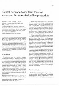
K. Patan et al. two hidden layers should be implemented. ANNs are parallel data processing tools capable of learning functional dependencies of the data. This feature is extremely useful for solving various pattern recognition problems. Another attractive property is the self-learning ability. A neural network can extract the system features from historical training data using a learning algorithm, requiring little or no a priori knowledge about the process. This makes ANNs nonlinear modelling tools of a great flexibility. Neural networks are also robust with respect to incorrect or missing data. Protective relaying based on ANNs is not affected by a change in the system operating conditions. Neural networks also have high computation rates, substantial input error tolerance and adaptive capability. These features allow applying neural networks effectively to the modelling and identification of complex nonlinear dynamic processes and fault diagnosis (Marcu et al., 1999; Patan and Parisini, 2005). 2.1. Locally recurrent neural network. Let us consider a discrete-time neural network with n inputs and m outputs. The network structure is composed of two processing layers with v1 neurons with Infinite Impulse Response (IIR) filters in the first layer and v2 neurons with Finite Impulse Response (FIR) filters in the second layer. Each neuron consists of a filter of order r. The state of such a network is represented as follows: (1a) x1 (k + 1) = A1 x1 (k) + W 1 u(k),  1 1 1 2 2 2 2 x (k + 1) = A x (k) + W σ G2 (B x (k)  +D 1 u(k) − g 11 ) + W u u(k), (1b) where x1 (k) ∈ RN1 (N1 = v1 × r) represents the states of the first layer and x2 (k) ∈ RN2 (N2 = v2 × r) represents the states of the second layer, A1 ∈ RN1 ×N1 and A1 ∈ RN2 ×N2 are the block diagonal state matrices of the first and second layers, respectively, W 1 ∈ RN1 ×n is the input weight matrix, W 2 ∈ RN2 ×v1 is the weight matrix between the first and second layers, W u ∈ RN2 ×n is the weight matrix between the input and the second layer, B 1 ∈ Rv1 ×N1 is the block diagonal matrix of feedforward filter parameters of the first layer, D 1 ∈ Rv1 ×n is the transfer matrix, g 11 denotes the vector of biases of the first layer, G12 ∈ Rv1 ×v1 is the diagonal matrix of the slope parameters of the first layer, and σ : Rv1 → Rv1 is a nonlinear vector-valued function. A detailed form of the network matrices can be found in (Patan, 2008). Neurons of the second layer receive excitation not only from the neurons of the previous layer, but also from the external inputs (Fig. 1). The first layer includes neurons with IIR filters while the second one consists of neurons with FIR filters. In this case, the second layer of the network is not a hidden one, contrary to the original structure of locally recurrent networks (Patan and

Towards robustness in neural network based fault diagnosis Parisini, 2005). The following result presents approximation abbilities of the modified neural network: Theorem 1. (Patan, 2007a) Let S ∈ Rn and U ∈ Rm be open sets, Ds ∈ S and Du ∈ U compact sets, Z ∈ Ds an open set, and f : S × U → Rn a C 1 vector-valued function. For a discrete-time nonlinear system of the form z(k + 1) = f (z(k), u(k)),

z ∈ R ,u ∈ R m

n

(2)

with an initial state z(0) ∈ Z, for arbitrary  > 0 and an integer 0 < I < +∞, there exist integers v1 and v2 as well as a neural network of the form (1) with an appropriate initial state x(0) such that for any bounded input u : R+ = [0, ∞] → Du max z(k) − x2 (k) < ε.

0≤k≤I

(3)

The network structure (1) is not a strict feedforward one, as it has a cascade structure. The introduction of an additional weight matrix W u renders it possible to obtain a system equivalent to the classical locally recurrent network with two hidden layers (Patan and Parisini, 2005), but the main advantage of this representation is that the whole state vector is available from the neurons of the second layer of the network. This fact is of crucial importance taking into account the training of the neural network. If the output y(k) is y(k) = x2 (k),

(4)

then weight matrices can be determined using a training process, which minimizes the error between the network output and measurable process states. Usually, in engineering practice, not all process states are directly available (measurable). In such cases, the dimension of the output vector is rather lower than the dimension of the state vector, and the network output can be produced in the following way: 2

y(k) = Cx (k).

(5)

In such cases, the cascade neural network contains an additional layer of static linear neurons playing the role of the output layer (Fig. 1). 2.2. Robustness via model error modelling. A robust identification procedure should deliver not only a model of a given process, but also a reliable estimate of the uncertainty associated with the model. Two main ideas exist to deal with the uncertainty associated with the model. The first group of approaches, the so-called set membership identification (Milanese, 2004; Duzinkiewicz, 2006) or bounded error approaches (Walter and Pronzato, 1997), relies on the assumption that the identification error is unknown but bounded. In this framework, robustness is

445 l– neuron with the IIR filter IIR

Ll– static linear neuron

l– neuron with the FIR filter FIR IIR FIR IIR

u(k)

y1 (k) L

y2 (k)

FIR L FIR

Fig. 1. Cascade structure of the modified dynamic neural network.

hardly integrated with the identification process. A somewhat different approach is to identify the process without robustness deliberations first, and then consider robustness as an additional step. This usually leads to least squares estimation and prediction error methods. Model Error Modelling (MEM) employs prediction error methods to identify a model from input-output data (Reinelt et al., 2002). After that, one can estimate the uncertainty of the model by analyzing residuals evaluated from the inputs. Uncertainty is a measure of unmodelled dynamics, noise and disturbances. The identification of residuals provides the so-called error model. In the original algorithm, a nominal model along with uncertainty is constructed in the frequency domain adding frequency by frequency the model error to the nominal model (Reinelt et al., 2002). Below, an algorithm to form uncertainty bands in the time domain is proposed, intended for use in the fault diagnosis framework (Patan et al., 2007). The design procedure is described by the following steps: 1. Using a model of the process, compute the residual r = y − ym , where y and ym are desired and model outputs, respectively. 2. Collect the data {ui , ri }N i=1 and identify an error model using these data. This model constitutes an estimate of the error due to undermodelling, and it is called the error model. 3. Derive the centre of the uncertainty region as ym +ye . 4. If the model error model is not falsified by the data, one can use statistical properties to calculate a confidence region. A confidence region forms uncertainty bands around the response of the error model. The model error modelling scheme can be carried out by using neural networks of the dynamic type. Both the fundamental model of the process and the error model can be modelled utilizing such networks. Assuming that the fundamental model of the process has already been constructed, the next step is to design the error model. In this

K. Patan et al.

446 case, a neural network is used to model an “error” system with input u and output r. After training, the response of this model is used to form uncertainty bands, where the centre of the uncertainy region is obtained as a sum of the output of the system model and the output of the error model. Then, the upper band can be calculated as Tu = ym + ye + tβ v,

(6)

and the lower band in the following way: Tl = ym + ye − tβ v,

(7)

where ye is the output of the error model on the input u, tβ is the N (0, 1) tabulated value assigned to a given confidence level, e.g, β = 0.05 or β = 0.01, v is the standard deviation of ye . It should be kept in mind that ye represents not only a residual but also structured uncertainty, disturbances, etc. Therefore, the uncertainty bands (6) and (7) should work well only assuming that the signal ye has a normal distribution. The centre of the uncertainty region is the signal ym + ye ≈ y. Now, observing the system output y, one may make a decision whether or not a fault occurred. If y is inside the uncertainty region, the system is healthy. 2.3. Robust GMDH neural networks. Successful application of ANNs in system identification and fault diagnosis tasks (Witczak, 2006) depends on a proper selection of the neural network architecture. In the case of classical ANNs such as MLPs, the problem reduces to the selection of the number of layers and the number of neurons in a particular layer. If the obtained network does not satisfy prespecified requirements, then a new network structure is selected and the parameter estimation is repeated once again. The determination of the appropriate structure and parameters of the model in the presented way is a complex task. Furthermore, an arbitrary selection of the ANN structure can be a source of model uncertainty. Thus, it seems desirable to have a tool which can be employed for automatic selection of the ANN structure, based only on the measured data. To overcome this problem, GMDH neural networks (Ivakhnenko and Mueller, 1995; Witczak et al., 2006) have been proposed. The synthesis process of a GMDH model is based on iterative processing of a sequence of operations. This process leads to the evolution of the resulting model structure in such a way as to obtain the best quality approximation of the identified system. Thus, the task of designing a neural network is defined in such a way as to obtain a model with a small uncertainty. The idea of the GMDH approach rests on replacing the complex neural model by a set of hierarchically connected neurons. The behaviour of each neuron should reflect the behaviour of the modelled system. From the rule of the GMDH algorithm it follows that the parameters of each neuron are estimated in such a way that their output

signals are the best approximation of the real system output. In this situation, the neuron should have an ability to represent the dynamics. One way out of this problem is to use dynamic neurons (Patan and Parisini, 2005). Dynamics in this neuron are realized by introducing a linear dynamic system—an IIR filter. The process of GMDH network synthesis leads to the evolution of the resulting model structure in such a way as to obtain the best quality approximation of the real system. An outline of the GMDH algorithm can be as follows (Witczak et al., 2006): Step 1: Determine all neurons (estimate their parameter (l) vectors pn with the training data set T ) whose inputs consist of all possible couples of input variables, i.e., (r − 1)r/2 couples, where r is the dimension of the system input vector. Step 2: Using a validation data set V, not employed during the parameter estimation phase, select several neurons which are best fitted in terms of the chosen criterion. Step 3: If the termination condition is fulfilled (either the network fits the data with a desired accuracy, or the introduction of new neurons did not induce a significant increase in the approximation abilities of the neural network), then STOP. Otherwise, use the outputs of the best-fitted neurons (selected in Step 2) to form the input vector for the next layer, and then go to Step 1. To obtain the final structure of the network, all unnecessary neurons are removed, leaving only those which are relevant to the computation of the model output. The procedure of removing the unnecessary neurons is the last stage of the synthesis of the GMDH neural network. The appealing feature of the above algorithm is that the techniques for parameter estimation of linear-in-parameter models can be used during the realization of Step 1. This is possible under the standard invertibility assumption of the activation function of a network. 2.3.1. Confidence estimation of GMDH neural networks. Even though the application of the GMDH approach to model structure selection can improve the quality of the model, the resulting structure is not the same as that of the system. It can be shown (Mrugalski, 2004) that the application of the classic evaluation criteria like the Akaike Information Criterion (AIC) and the Final Prediction Error (FPE) (Ivakhnenko and Mueller, 1995; Mueller and Lemke, 2000) can lead to the selection of inappropriate neurons and, consequently, to unnecessary structural errors. Apart from the model structure selection stage, inaccuracy in parameter estimates also contributes to modelling uncertainty. Indeed, while applying the leastsquare method to parameter estimation of neurons, a set

Towards robustness in neural network based fault diagnosis of restrictive assumptions has to be satisfied (see, e.g., (Witczak et al., 2006) for further explanations). An effective remedy to such a challenging problem is to use the so-called Bounded Error Approach (BEA) (Milanese et al., 1996; Witczak et al., 2006). Let us consider the following system: y(k) = r(k)T p + ε(k),

(8)

where r(k) stands for the regressor vector, p ∈ Rnp denotes the parameter vector, and ε(k) represents the difference between the original system and the model. The ˆ , as well problem is to obtain a parameter estimate vector p as an associated parameter uncertainty required to design robust fault detection system. The knowledge regarding the set of admissible parameter values allows obtaining the confidence region of the model output which satisfies y˜m (k) ≤ y(k) ≤ y˜M (k),

(9)

where y˜m (k) and y˜M (k) are respectively the minimum and maximum admissible values of the model output that are consistent with the input-output measurements of the system. It is assumed that ε(k) consists of a structural deterministic error caused by the model-reality mismatch, and the stochastic error caused by the measurement noise is bounded as follows: εm (k) ≤ ε(k) ≤ εM (k),

(10)

where the bounds εm (k) and εM (k) (εm (k) = εM (k)) can be estimated (Witczak et al., 2006). The idea underlying the bounded error approach is to obtain a feasible parameter set P (Milanese et al., 1996) that is consistent with the input-output measurements used for parameter estimation. The resulting P is described by a polytope defined by a set of vertices V. Thus, the problem of determining model output uncertainty can be solved as follows: r T (k)pm (k) ≤ r T (k)p ≤ r T (k)pM (k),

(11)

where pm (k) = arg min r T (k)p, p∈V

p (k) = arg max r T (k)p. M

(12)

p∈V

As has been mentioned, the neurons in the l-th (l > 1) layer are fed with the outputs of the neurons from the (l − 1)-th layer. In order to modify the above approach for the uncertain regressor case, let us express the unknown “true” value of the regressor r n (k) by a difference between a measured value of the regressor r(k) and the error in the regressor e(k): r n (k) = r(k) − e(k),

(13)

where it is assumed that the error e(k) is bounded as M em i (k) ≤ ei (k) ≤ ei (k),

i = 1, . . . , np .

(14)

447 Using (8) and substituting (13) into (14), one can define the space containing the parameter estimates: εm (k) − eT (k)p ≤ y(k) − r(k)T p ≤ εM (k) − eT (k)p, (15) which makes it possible to adapt the above-described technique to the error-in-regressor case (Witczak et al., 2006). The proposed modification of the BEA makes it possible to estimate the parameter vectors of the neurons from the l-th layer, l > 1. Finally, it can be shown that the model output uncertainty has the following form: y˜m (k) ≤ r Tn p ≤ y˜M (k).

(16)

In order to adapt the presented approach to the parameter estimation of nonlinear neurons with an activation function ξ(·), it is necessary to transform the relation   T (17) εm (k) ≤ y(k) − ξ (r(k)) p ≤ εM (k), using ξ −1 (·), and hence   T ξ −1 y(k) − εM (k) ≤ (r(k)) p ≤ ξ −1 (y(k) − εm (k)) .

(18)

Knowing the model structure and possessing the knowledge regarding its uncertainty, it is possible to design a robust fault detection scheme with an adaptive threshold. The model output uncertainty interval, calculated with the application of the GMDH model, should contain the real system response in the fault-free mode. Therefore, the system output should satisfy y˜m (k) + εm (k) ≤ y(k) ≤ y˜M (k) + εM (k).

(19)

This means that robust fault detection boils down to checking if the output of the system satisfies (19). Thus, when (19) is violated, a fault symptom occurs. 2.4. Theoretical comparison. The main objective of this section is to compare the design techniques and the resulting neural network fault diagnosis schemes presented in Section 2. In general, the design techniques described in Sections 2.1 and 2.3 lead to the same type of a neural network, i.e., a feedforward neural network with dynamic neuron models. The main difference is that the GMDH network structure (Secton 2.3) is selected automatically while the structure of a network described in Section 2.1 is arbitrarily selected. Another crucial difference is that the parameters of GMDH neurons are estimated independently while in the case of the network described in Section 2.1 this is realized simultaneously. This means that the parameter vector associated with a neuron is optimal for this particular neuron only. On the other hand, this parameter vector may not be optimal from the point of view of the entire network. Such circumstances

K. Patan et al.

448 rise the need for the retraining of the GMDH neural network after the automatic selection of the model structure. This leads directly to an obvious equivalence between the above-mentioned procedures, which makes their empirical comparison senseless. A similar line of reasoning can be realized for the adaptive threshold determination techniques described in Sections 2.2 and 2.3.1. In particular, in the first case a neural network is used to determine the interval containing the possible system response, while in the second case the output interval is determined with the knowledge about the parameter uncertainty of a neural model of the system. As can be shown (Witczak, 2007), the performance of such techniques strongly depends on the experimental conditions employed during the design procedure. In other words, a direct answer regarding the superiority of one of these technique cannot be formulated, which makes their empirical comparison senseless. Thus, they should be perceived as two alternative design procedures. Therefore, in the further part of the paper, the model error modelling procedure is applied to design the FDI system for a DC motor.

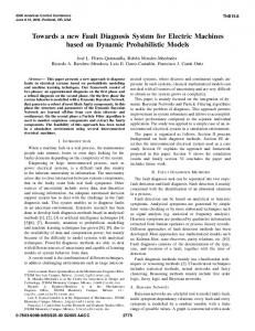
In this section, robust model based fault diagnosis of the AMIRA DR300 laboratory system is presented. The laboratory system shown in Fig. 2 is used to control the rotational speed of a DC motor with a changing load. The laboratory object considered consists of five main elements: a DC motor M1, a DC motor M2, two digital increamental encoders and a clutch K. The input signal of the engine M1 is an armature current and the output one is the angular velocity. The available sensors for the output are an analog tachometer on an optical sensor, which generates impulses that correspond to the rotations of the engine, and a digital incremental encoder. The shaft of the motor M1 is connected with the identical motor M2 by the clutch K. The second motor M2 operates in the generator mode and its input signal is an armature current. The available measuremets of the plant are as follows:

3. Neural network based fault diagnosis of a DC motor

and control signals include:

Electrical motors play a very important role in safe and efficient work of modern industrial plants and processes. Early diagnosis of abnormal and faulty states renders it possible to perform important preventing actions, and it allows one to avoid heavy economic losses involved in stopped production, or the replacement of elements or parts (Chen and Patton, 1999). To keep an electrical machine in the best condition, several techniques such as fault monitoring or diagnosis should be implemented. Conventional DC motors are very popular, because they are reasonably cheap and easy to control. Unfortunately, their main drawback is the mechanical collector, which has only a limited life span. In addition, brush sparking can destroy the rotor coil, generate electromagnetic compatibility problems and reduce insulation resistance to an unacceptable limit (Moseler and Isermann, 2000). Moreover, in many cases, electrical motors operate in closed-loop control and small faults often remain hidden by the control loop. It is only if the whole device fails that the failure becomes visible. Therefore, there is a need to detect and isolate faults as early as possible. Recently, a great deal of attention has been paid to electrical motor fault diagnosis (Nandi et al., 2005; Li et al., 2004; Moseler and Isermann, 2000; Xiang-Qun and Zhang, 2000; Fuessel and Isermann, 2000). In general, the elaborated solutions can be splitted into three categories: signal analysis methods, knowledge based methods and model based approaches (Xiang-Qun and Zhang, 2000; Korbicz et al., 2004).

• motor current Im – the motor current of the DC motor M1, • generator current Ig – the motor current of the DC motor M2, • tachometer signal T , • motor control signal Cm – the input of the motor M1, • generator control signal Cg – the input of the motor M2. The separately excited DC motor is governed by two differential equations. The classical description of the electrical subsystem is given by the equation u(t) = Ri(t) + L

di(t) + e(t), dt

(20)

where u(t) is the motor armature voltage, R is the armature coil resistance, i(t) is the motor armature current, L is the motor coil inductance, and e(t) is the induced electromotive force. The counter electromotive force is proportional to the angular velocity of the motor: e(t) = Ke ω(t),

Fig. 2. Laboratory system with a DC motor.

(21)

Towards robustness in neural network based fault diagnosis where Ke stands for the motor voltage constant and ω(t) is the angular velocity of the motor. In turn, the mechanical subsystem can be derived from a torque balance: dω(t) = Tm (t) − Bm ω(t) − Tl − Tf (ω(t)), dt

(22)

where J is the motor moment of inertia, Tm is the motor torque, Bm is the viscous friction torque coefficient, Tl is the load torque, and Tf (ω(t)) is the friction torque. The motor torque Tm (t) is proportional to the armature current Tm (t) = Km i(t),

linear activation functions, and one linear output neuron (Patan, 2007b; Patan et al., 2007). The neural model structure was selected using the “trial and error” method. The quality of each model was determined using the Akaike Information Criterion (AIC) (Ljung, 1999). This criterion contains a penalty term and makes it possible to discard too complex models. The training process was carried out for 100 steps using the Adaptive Random Search (ARS) algorithm (Walter and Pronzato, 1997; Patan and Parisini, 2002) with the initial variance v0 = 0.1.

(23)

where Km stands for the motor torque constant. The friction torque can be considered as a function of the angular velocity and it is assumed to be the sum of the Stribeck, Coulumb and viscous components. The viscous friction torque opposes motion and it is proportional to the angular velocity. The Coulomb friction torque is constant at any angular velocity. The Stribeck friction is a nonlinear component occuring at low angular velocities. Although the model (20)–(23) has a direct relation to the motor physical parameters, the true relation between them is nonlinear. There are many nonlinear factors in the motor, e.g., the nonlinearity of the magnetization characteristic of the material, the effect of material reaction, the effect caused by an eddy current in the magnet, residual magnetism, the commutator characteristic, mechanical frictions (XiangQun and Zhang, 2000). These factors are not shown in the model (20)–(23). Summarizing, the DC motor is a nonlinear dynamic process, and to model it suitably nonlinear modelling, e.g., dynamic neural networks (Patan, 2007a), should be employed. The motor described works in closed-loop control with the PI controller. It is assumed that the load of the motor is zero. The objective of system control is to keep the rotational speed at the constant value equal to 2000. Additionally, it is assumed that the reference value is corrupted by additive white noise.

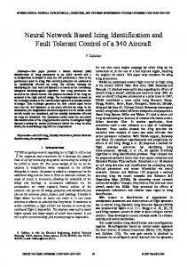
Decision making. To estimate the uncertainty associated with the neural model, the MEM technique, discussed in Section 2.2, is applied. To design the error model, the classical linear ARX model is utilized. In order to select a proper number of delays, several ARX models were examined and the best performing one was selected using the AIC. The parameters of the ARX model were the number of past outputs na = 20 and the number of past outputs nb = 20. The sum of squared errors calculated for 3000 20 15

Residual and thresholds

J

449

10 5 0 −5 −10 −15 1000

1100

1200

1300

1400

1500

1400

1500

Discrete time

(a) 2050 2040

The following input signal was used in the experiments: Cm (k) =3 sin(2π1.7k) + 3 sin(2π1.1k − π/7) + 3 sin(2π0.3k + π/3).

(25)

The input signal (25) is persistantly exciting of order 6 (Ljung, 1999). Using (25), a learning set containig 1000 samples was formed. The neural network model (1) and (5) had the following structure: one input, three IIR neurons with first order filters and hyperbolic tangent activation functions, six FIR neurons with first order filters and

2030

Confidence bands

Motor modelling. A separately excited DC motor was modelled by using the dynamic neural network (1) proposed in Section 2.1. The model of the motor was selected as follows: (24) T = f (Cm ).

2020 2010 2000 1990 1980 1970 1960 1000

1100

1200

1300

Discrete time

(b) Fig. 3. Residual and constant thresholds (a) and confidence bands generated by model error modelling (b).

K. Patan et al.

450

• fi2 – mechanical faults were simulated by increasing/decreasing motor torque, in turn by ±20%, ±10% and ±5%.

2050

Confidence bands

2000

1950

1900

1850

1800 3700

3800

3900

4000

4100

4200

4300

4400

Discrete time

(a) 1.5

Decision making

1

0.5

0

−0.5 3700

3800

3900

4000

4100

4200

4300

4400

Discrete time

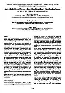
(b) Fig. 4. Fault detection using model error modelling: fault f11 – confidence bands (a) and decision logic without the time window (b).

testing samples for the ARX model was equal to 0.0117. Using the procedure described in Section 2.2 and assuming the confidence level equal to β = 0.05, two bands were calculated. The results are presented in Fig. 3(b). To evaluate the quality of the proposed solution, another decision making technique based on constant thresholds is also applied (Patan and Parisini, 2005). Decision making using constant thresholds is illustrated in Fig. 3(a). In both methods, a number of false alarms represented by the false detection rate rf d was monitored (Patan and Parisini, 2005). The achieved indices are rf d = 0.012 in the case of adaptive thresholds and rf d = 0.098 in the case of constant ones. Fault detection. Two types of faults were examined during the experiments: • fi1 – tachometer faults were simulated by increasing/decreasing rotational speed, in turn by ±20%, ±10% and ±5%,

As a result, a total of 12 faulty situations were investigated. Each fault occurred at the tf rom = 4000 time step and lasted to the ton = 5000 time step. In order to perform a decision about the faults and to determine the detection time tdt , a time window with the length 0.25 s was used. The results of the fault detection are presented in Table 1. All faults were reliably detected using model error modelling, contrary to the constant threshold technique. In the latter case, problems were encountered with the faults f41 , f52 and f62 (marked with boxes). An interesting situation is observed for the fault f61 . Due to the moving window with the length of 50, false alarms were not raised just before the 4000-th time step, but in practice from the 3968th time step the residual exceeded the threshold, which means a false alarm. Summarizing, the MEM technique demonstrates more reliable behaviour than simple thresholding. The example of fault detection is illustrated in Fig. 4 for the case of adaptive thresholds. Fault isolation. Fault isolation can be considered as a classification problem where a given residual value is assigned to one of the predefined classes of system behaviour. In the case considered here, there is only one residual signal and 12 different faulty scenarios. Firstly, it is required to check the distribution of the symptom signals in order to verify the separability of the faults. The symptom distribution is shown in Fig. 5. Almost all classes are separable except the faults f11 (marked with ‘o’) and f62 (marked with ‘∗’), which overlap each other. A similar situation is observed for the faults f21 (marked with ‘·’) and f52 (marked with ‘+’). As a result, the pairs f11 , f62 , and f21 , f32 can be isolated, but as a group of faults only. Finally, 10 classes of faults are formed: C1 = {f11 , f62 }, C2 = {f21 , f52 }, C3 = {f31 }, C4 = {f41 }, C5 = {f51 }, C6 = {f61 }, C7 = {f12 }, C8 = {f22 }, C9 = {f32 } and C10 = {f42 }. To perform fault isolation, the well-known multilayer perceptron was used. The neural network had two inputs (the model input and the residual) and four outputs (each class of the system behaviour was coded using a 4-bit representation). The learning set was formed using 100 samples per each faulty situation, then the size of the learning set was equal to 1200. As the well-performing neural classifier, the network with 15 hyperbolic tangent neurons in the first hidden layer, ten hyperbolic tangent neurons in the second hidden layer, and four sigmoidal output neurons was selected. The neural classifier was trained for 200 steps using the LevenbergMarquardt method. Additionally, the real-valued response of the classifier was transformed to the binary one. A simple idea is to calculate the distance between the classifier output and each predefined class of system behaviour. As

Towards robustness in neural network based fault diagnosis

451

Table 1. Results of fault detection for model error modelling. f11

f21

f31

f41

f51

f61

97.9 4074

99.6 4055

98.8 4077

99.7 4053

99.6 4058

99.5 4075

98.1 4072

99.4 4067

98.8 4064

99.4 3147

98.9 4063

100 4018

f12

f22

f32

f42

f52

f62

99.2 4058

99.3 4100

99.2 4060

98.8 4061

99.1 4060

81 4357

99.5 4056

99.7 4059

99.3 4057

99.1 4059

99.9 3726

98.4 3132

Model error modelling rtd [%] tdt Constant thresholds rtd [%] tdt

Model error modelling rtd [%] tdt Constant thresholds rtd [%] tdt

a result, the binary representation giving the shortest Euclidean distance is selected as the classifier binary output. This transformation can be represented as follows: j = arg min||x − Ki ||, i

i = 1, . . . , NK ,

(26)

where x is the real-valued output of the classifier, Ki is the binary representation of the i-th class, NK is the number of predefined classes of system behaviour, and || · || is the Euclidean distance. Then, the binary representation of the classifier can be determined in the form x ¯ = Kj . Recognition accuracy (R) results are presented in Table 2. All classes of faulty situations were recognized surely with accuracy greater than 90%. True values of recognition accuracy are marked with boxes. There are situations of misrecognizing, e.g., the class C4 was classified as the class C2 with the rate 5.7%. Misrecognizing can be caused by the fact that some classes of faults are closely arranged in the symptom space or even slightly overlap each other. Such a situation is observed for the classes C4 and C9 . Generally speaking, the achieved isolation results are satisfactory. It is neccesary to mention that such high isolation rates are only achievable if some faulty scenarios can be treated as a group of faults. In the case considered, there were two such groups of faults, C2 and C1 . Fault identification. In this experiment, the objective of fault identification was to estimate the size (S) of detected and isolated faults. When analytical equations of residuals are unknown, fault identification consists in estimating the fault size and the time of fault occurrence on the basis of residual values. An elementary index of the residual size assigned to the fault size is the ratio of the residual value

rj to a suitably assigned threshold value Tj . In this way, the fault size can be represented as the mean value of such elementary indices for all residuals as follows: S(fk ) =

1 N

 j:rj ∈R(fk )

rj , Tj

(27)

where S(fk ) represents the size of the fault fk , R(fk ) is the set of residuals sensitive to the fault fk , N is the size of the set R(fk ). The threshold values are given at the beginning of this section. The results are shown in Table 3. Analyzing them, one can observe that quite large values were obtained for the faults f51 , f61 and f12 . These faults were arbitrarily assigned to the group large. Another group is formed by the faults f31 , f41 , f22 , f32 and f42 , possessing similar values of the fault size. This group was called medium. The third group of faults consists of f11 , f21 , f52 and f62 . The fault sizes in these cases are distinctly smaller than in the cases already discussed, and this group is called small. The small size of the faults f52 and f62 somewhat explains problems with their detection using a constant threshold (see Table 3).

4. Conclusions The paper discusses neural network based methods for robust fault diagnosis. Both methods considered give a prescription how to estimate the uncertainty of a neural network composed of dynamic neuron models. The first method, model error modelling, makes it possible to obtain a description of an existing neural model, which then can be used for robust fault diagnosis, while the second approach, the robust GMDH neural network, renders it

K. Patan et al.

452

400

f11 f21 f31 f41 f51 f61

300

200

f12 f22 f32 f42 f52 f62

Residual

100

0

−100

−200

−300

−400 0.16

0.18

0.2

0.22

0.24

0.26

0.28

0.3

0.32

0.34

0.36

System input

Fig. 5. Symptom distribution.

Table 2. Fault isolation results. R [%] C1

C2

C3

C4

C5

C6

C7

C8

C9

C10

f11 f21 f31 f41 f51 f61 f12 f22 f32 f42 f52 f62

– 99.7 0.5 5.7 – 0.2 – – – 0.7 97.7 2.5

– – 99.3 0.7 – – – – 0.2 3.0 – –

– – – 93.6 0.9 – – – 3.9 – – –

– – – – 94.1 1.1 0.4 – – – – –

– – – – – 95.9 1.4 – – – – –

– – – – 0.5 – 97.5 1.6 – – – –

– – – – – – – 98.4 1.8 – – –

– – – – – 2.1 0.7 – 94.1 2.1 – –

– – – – 3.4 0.7 – – – 94.1 2.3

100 0.3 0.2 – 0.9 – – – – 0.2 – 97.5

Table 3. Fault identification results. S

f11

small 2.45 medium large

f21 3.32

f31

f41

5.34

6.19

f51

10.9

f61

11.64

f12

17.39

f22

f32

f42

8.27

8.61

8.65

f52

f62

2.28

1.73

Towards robustness in neural network based fault diagnosis possible to obtain a model with a possibly small uncertainty as well as to estimate its uncertainty, which then can be used for robust fault diagnosis. The characteristics and a comparison of both methods are provided in Section 2.4. The paper also presents experimental studies including robust fault detection, fault isolation and fault identification of a DC motor. Using the novel cascade structure of the dynamic neural network, quite an accurate model of the motor was obtained which can mimic a technological process with a pretty good accuracy. It was shown that the proposed robust fault diagnosis procedure carried out by using model error modelling significantly reduces the number of false alarms caused by an inaccurate model of the process. Due to the estimation of model uncertainty, the robust fault diagnosis system may be much more sensitive to the occurrence of small faults than standard decision making methods such as constant thresholds. The supremacy of MEM may be evident in the case of incipient faults, when a fault develops very slowly and a robust technique performs in a more sensitive manner that constant thresholds. Moreover, comparing false detection ratios calculated for normal operating conditions for adaptive as well as constant thresholds, one can conclude that the number of false alarms was considerably reduced when model error modelling was applied. Furhermore, fault isolation was performed using the standard multi-layer perceptron. Preliminary analysis of the symptom distribution and splitting faulty scenarios into groups make it possible to obtain high fault isolation rates. The last step in the fault diagnosis procedure was fault identification. In its framework, the objective was to estimate the fault size. This was done by checking how much the residual exceeded the threshold assigned to it. The whole fault diagnosis approach was successfully tested on a number of faulty scenarios simulated on a real plant, and the achieved results confirm the usefulness and effectiveness of artificial neural networks in designing fault detection and isolation systems. It should be pointed out that the presented solution can be easily applied to online fault diagnosis.

Acknowledgments This work was supported in part by the Ministry of Science and Higher Education in Poland under the grants N N514 1219 33 and R01 012 02 (DIASTER).

References Blanke M., Kinnaert M., Lunze J. and Staroswiecki M. (2003). Diagnosis and Fault-Tolerant Control, Springer, New York, NY. Chen J. and Patton R. J. (1999). Robust Model-Based Fault Diagnosis for Dynamic Systems, Kluwer, Berlin.

453 Duzinkiewicz K. (2006). Set membership estimation of parameters and variables in dynamic networks by recursive algorithms with a moving measurement window, International Journal of Applied Mathematics and Computer Science 16(2): 209–217. Frank P. M. and Köppen-Seliger B. (1997). New developments using AI in fault diagnosis, Engineering Applications of Artificial Intelligence 10(1): 3–14. Fuessel D. and Isermann R. (2000). Hierarchical motor diagnosis utilising structural knowledge and a self-learning neurofuzzy scheme, IEEE Transactions on Industrial Electronics 47(5): 1070–1077. Gertler J. (1998). Fault Detection and Diagnosis in Engineering Systems, Marcel Dekker, New York, NY. Haykin S. (1999). Neural Networks. A Comprehensive Foundation, 2nd Ed., Prentice-Hall, Englewood Cliffs, NJ. Iserman R. (2006). Fault Diagnosis Systems. An Introduction from Fault Detection to Fault Tolerance, Springer, New York, NY. Ivakhnenko A. G. and Mueller J. A. (1995). Self-organizing of nets of active neurons, System Analysis Modelling Simulation 20(2): 93–106. Köppen-Seliger B. and Frank P. M. (1999). Fuzzy logic and neural networks in fault detection, in L. Jain and N. Martin (Eds.), Fusion of Neural Networks, Fuzzy Sets, and Genetic Algorithms, CRC Press, New York, NY, pp. 169–209. Korbicz J. (2006). Fault detection using analytical and soft computing methods, Bulletin of the Polish Academy of Sciences: Technical Sciences 54(1): 75–88. Korbicz J., Ko´scielny J., Kowalczuk Z. and Cholewa W. (2004). Fault Diagnosis. Models, Artificial Intelligence, Applications, Springer, Berlin. Korbicz J., Patan K. and Kowal M. (Eds.) (2007). Fault Diagnosis and Fault Tolerant Control, Academic Publishing House EXIT, Warsaw. Li L., Mechefske C. K. and Li W. (2004). Electric motor faults diagnosis using artificial neural networks, Insight: Non-Destructive Testing and Condition Monitoring 46(10): 616–621. Ljung L. (1999). System Identification—Theory for the User, Prentice Hall, Englewood Cliffs, NJ. Marcu T., Mirea L. and Frank P. M. (1999). Development of dynamical neural networks with application to observer based fault detection and isolation, International Journal of Applied Mathematics and Computer Science 9(3): 547–570. Milanese M. (2004). Set membership identification of nonlinear systems, Automatica 40(6): 957–975. Milanese M., Norton J., Piet-Lahanier H. and Walter E. (1996). Bounding Approaches to System Identification, Plenum Press, New York, NY. Moseler O. and Isermann R. (2000). Application of model-based fault detection to a brushless DC motor, IEEE Transactions on Industrial Electronics 47(5): 1015–1020.

454 Mrugalski M. (2004). Neural Network Based Modelling of Nonlinear Systems in Fault Detection Schemes., Ph.D. thesis, University of Zielona Góra, (in Polish). Mueller J. E. and Lemke F. (2000). Self-Organising Data Mining, Libri, Hamburg.

K. Patan et al. Patan K. and Parisini T. (2005). Identification of neural dynamic models for fault detection and isolation: The case of a real sugar evaporation process, Journal of Process Control 15(1): 67–79.

Nandi S., Toliyat H. A. and Li X. (2005). Condition monitoring and fault diagnosis of electrical motors—A review, IEEE Transactions on Energy Conversion 20(4): 719–729.

Puig V., Stancu A., Escobet T., Nejjari F., Quevedo J. and Patton, R. J. (2006). Passive robust fault detection using interval observers: Application to the DAMADICS benchmark problem, Control Engineering Practice 14(6): 621–633.

Narendra K. S. and Parthasarathy K. (1990). Identification and control of dynamical systems using neural networks, IEEE Transactions on Neural Networks 1(1): 12–18.

Reinelt W., Garulli A. and Ljung L. (2002). Comparing different approaches to model error modeling in robust identification, Automatica 38(5): 787–803.

Nelles O. (2001). Nonlinear System Identification. From Classical Approaches to Neural Networks and Fuzzy Models, Springer-Verlag, Berlin.

Rodrigues M., Theilliol D., Aberkane S. and Sauter D. (2007). Fault tolerant control design for polytopic LPV systems, International Journal of Applied Mathematics and Computer Science 17(1): 27–37.

Norgard M., Ravn O., Poulsen N. and Hansen L. (2000). Networks for Modelling and Control of Dynamic Systems, Springer, London. Patan K. (2007a). Approximation ability of a class of locally recurrent globally feed-forward neural networks, Proceedings of the European Control Conference, ECC 2007, Kos, Greece, published on CD-ROM. Patan K. (2007b). Robust faul diagnosis in a DC motor by means of artificial neural networks and model error modelling, in J. Korbicz, K. Patan and M. Kowal (Eds.), Fault Diagnosis and Fault Tolerant Control, Academic Publishing House EXIT, Warsaw, pp. 337–346. Patan K. (2007c). Stability analysis and the stabilization of a class of discrete-time dynamic neural networks, IEEE Transactions on Neural Networks 18(3): 660–673. Patan K. (2008). Aproximation of state-space trajectories by locally recurrent globally feed-forward neural networks, Neural Networks 21(1): 59–64. Patan K., Korbicz J. and Głowacki G. (2007). DC motor fault diagnosis by means of artificial neural networks, Proceedings of the 4th International Conference on Informatics in Control, Automation and Robotics, ICINCO 2007, Angers, France, published on CD-ROM. Patan K. and Parisini T. (2002). Stochastic learning methods for dynamic neural networks: Simulated and real-data comparisons, Proceedings of the 2002 American Control Conference, ACC’02, Anchorage, AK, USA, pp. 2577–2582.

Rutkowski L. (2004). New Soft Computing Techniques for System Modelling, Pattern Classification and Image Processing, Springer, Berlin. Walter E. and Pronzato L. (1997). Identification of Parametric Models from Experimental Data, Springer, London. Witczak M. (2006). Advances in model-based fault diagnosis with evolutionary algorithms and neural networks, International Journal of Applied Mathematics and Computer Science 16(1): 85–99. Witczak M. (2007). Modelling and Estimation Strategies for Fault Diagnosis of Non-linear Systems, Springer, Berlin. Witczak M., Korbicz J., Mrugalski M. and Patton R. J. (2006). A GMDH neural network-based approach to robust fault diagnosis: Application to the DAMADICS benchmark problem, Control Engineering Practice 14(6): 671–683. Xiang-Qun L. and Zhang H. Y. (2000). Fault detection and diagnosis of permanent-magnet DC motor based on parameter estimation and neural network, IEEE Transactions on Industrial Electronics 47(5): 1021–1030. Received: 13 February 2008 Revised: 18 June 2008