Model Checking of Systems Employing Commutative Functions

Model Checking of Systems Employing Commutative Functions A. Prasad Sistla, Min Zhou, and Xiaodong Wang University of Illinois at Chicago

Abstract. The paper presents methods for model checking a class of possibly infinite state concurrent programs using various types of bi-simulation reductions. The proposed methods work for the class of programs in which the functions that update the variables are mutually commutative. A number of bi-simulation relations are presented for such systems. Explicit state model checking methods that employ on-the-fly reductions with respect to these bi-simulations are given. Some of these methods have been implemented and have been used to verify some well known protocols that employ integer variables. Various applications of the methods and optimization techniques for special cases are also given in appendix.

1

Introduction

Two of the bottlenecks that hinder wider applicability of model checking approach is the state explosion problem and its less effectiveness in handling infinite state systems. In this paper, we present an approach for model checking that works for certain classes of infinite state systems and that can also be used to contain the state explosion problem. One standard model checking method, employed often, is to construct the reachability graph of the given program and then check the correctness property against this graph. One way of reducing the size of the explored graph is to employ a reduction with respect to a bi-simulation relation U on the states of the reachability graph. Such a relation U is either known a priori through an implicit representation or has been computed by other means. In this paper, we give a method that does not require a priori computation of a bi-simulation relation. Instead, we give a sufficient condition on any two states to determine if they are bi-similar. This condition requires equivalence of certain predicates associated with the two states. In fact, we present a number of bi-simulation relations that can be used in on-the-fly model checking methods. Our approach works for certain classes of programs that employ commutative unary functions for updating variables. Since bi-similarity of two states is based on the future behavior from these states, in general, it is not possible to check their bi-similarity by looking only at the values of the variables in these states. We assume that the concurrent program is given by a Transition Diagram (TD) [11] which is an edge labeled directed graph. Each edge label consists of a condition, called guard, and an action which is a concurrent assignment of values to variables. We consider a class of TDs, called simple TDs, in which an expression that is assigned to a variable x is either a constant, or a variable, or of the form f (x) where f is a unary function. Further more, we require that the functions that are used be mutually commutative, that is, for any two functions f, g, f g = gf . (Note that such TDs are as powerful as Turing M/Cs). Our approach works as follows. First we preprocess the TD and compute a set of predicate templates with respect to each node q in the TD. (A predicate template is a predicate together with a function that renames some of its variables). These sets of predicate templates are computed, using a terminating fixpoint computation on the graph of the TD, from guards of the transitions of the TD and from predicates that appear in the correctness formula. In the second step, the reachability graph is constructed in a

symbolic form. Each of its states consists of a node in the TD and other components that give the values of the variables in symbolic form. We define an equivalence relation, ∼0 , on the states by instantiating the predicate templates associated with the corresponding TD node. Two states are equivalent if they are at the same TD node and the instantiations of the predicate templates in both the states are equivalent. We show that this equivalence relation is a bi-simulation. In general checking equivalence of predicates may require a theorem prover. However, for certain types of programs, such as those that use integer variables and additions of constants as functions, this equivalence can be checked efficiently if the predicates only involve standard comparison operators such as , etc. The requirements for the bi-simulation ∼0 can some times be too strong. In order for two symbolic states s, t at a node q to be related by ∼0 , we require that the instantiations, of each predicate template pt associated with q, in the states s and t be equivalent. Each such predicate template pt corresponds to a guard of a transition of the TD from some node r or to an atomic predicate in the correctness formula. Suppose that none of the guards of the transitions entering node r are ever satisfiable; then, we don’t need to require equivalence of the instantiations of pt with respect to both s and t because r will be never reached from either s or t. As a consequence, we can relax the equivalence requirement as follows. Suppose e is a transition entering the node r; then we require equivalence of the instantiations of pt only if the transition e is enabled with respect to both the states s and t. Thus we require conditional equivalence of template instantiations. The above relaxation in the requirement is done with respect to all the transitions entering node r and for every such node. The resulting binary relation ∼ 1 on symbolic states is also going to be a bi-simulation. The above notion of relaxing the requirement with respect to edges entering each node can be generalized to paths of length i entering each node.. When we do this, we get the relations ∼ i for each i > 0. The relation ∼0 , defined earlier, can be considered to be the relation when we consider paths of length zero, i.e. null paths, entering a node. We show that each ∼i is a bi-simulation and that ∼i ⊆∼i+1 for each i ≥ 0. Thus we get a chain of non-decreasing bi-simulations. For each i, we also show that there exists a TD for which ∼i is strictly contained in ∼i+1 . In fact, we can get a TD for which ∼i ⊂∼i+1 for every i ≥ 0. It is to be noted that using ∼i+1 gives us a smaller bi-simulation reduction, however there will be more conditional equivalence checks for ∼i+1 than for ∼i . We also show, in the appendix, that when we consider TDs over integer domain, i.e., when the variables range over integer and the functions that update variables only add constants, then we don’t need to use the symbolic graph and instead can use the standard reachability graph and define the bi-simulations on this graph. In all the above approaches, checking equivalence of predicates or conditional equivalence of predicates assumes an implicit universal quantification over their free variables. We show in appendix that by analyzing the TD in advance, i.e., by performing static analysis, the domain over which the universal quantifiers range can be reduced. (In fact, this domain itself can be defined by a formula.) This allows more states to be considered equivalent. When we do this over the symbolic graph, we get the bi-simulation relations ∼0i for each i ≥ 0. For TDs on the integer domains, as above, we can define these bi-simulations on the reachability graph itself. We show, in the appendix, that our techniques can be used to show decidability of the reachability problems for simple sub-classes of Hybrid automata [15, 19] when they are restricted to integer domains. All the above bi-simulations preserve correctness under fairness also. We have implemented the above methods and applied them to examples such as the sliding window protocol, etc. Experimental results showing the effectiveness of our approach are presented.

In summary, we have given methods based on bi-simulation reductions for model checking a class of TDs where the update functions satisfy certain commutativity conditions. We define a sequence of non-decreasing bi-simulations. These bi-simulations can be checked on-the-fly as the reachability graph is constructed. The methods employ static analysis for defining different predicate templates that are used for checking the bi-simulation of states. These bi-simulations preserve correctness under fairness, and hence the corresponding bi-simulation reductions can be used to verify both safety and liveness properties in their full generality. We also show some of the results of the paper can be used to prove the decidability of certain hybrid automata when restricted to the integer domains. Some of the proposed methods are implemented and have been used to verify real protocols. To the best our knowledge, this is the first time when these special types of TDs have been considered in a comprehensive manner and such a wide spectrum of bi-simulations are proposed and considered for model checking. The paper is organized as follows. Section 2 discusses applicability of the results of the paper and related work. Section 3 contains definitions and notation. Section 4 presents our method based on the bi-simulation relation ∼0 . Section 5 defines the bi-simulation relations with respect to paths of the TD, i.e. it defines the relations ∼i for i > 0 and presents results relating them. Section 6 presents experiment results. Section 7 contains conclusions. Section 8.1 in appendix presents extensions to the method. Section 8.2 in appendix shows how hybrid automata over discrete time domain can be handled and it also shows how the commutativity requirement can be relaxed. The proofs for theorems are given in section 8.3 in appendix.

2

Discussion and Related Work

The results of the paper are applicable to concurrent systems that can be modeled by simple TDs over any domain as described earlier. In particular, they can be applied to TDs over integer domains, i.e., where the variables range over integers and are updated by addition of constants and the predicates are of the form eρc where e is a linear combination of variables , ρ is a comparison relation and c is a constant. One class of integer TDs for which ∼0 gives a finite quotient of the reachability graph is where each expression appearing in the predicates has finite number of values in the reachability states, or each such expression is positive, i.e., all its coefficients are positive and all its variables are always incremented by positive constants. (It is to be noted that the case where each expression has only a finite number of values in the reachability state space can also be handled by considering a a new TD each of whose variable represents an expression in the original TD and is updated appropriately). The other cases where ∼0 gives finite quotients together with its applicability to hybrid automata over integer domains are given in the appendix. The bisimulations ∼i , for i > 0, give further reductions in the above cases and they also give finite quotients for some cases for which ∼0 does not give a finite quotient. Such examples are also given in the appendix (some as part of the proofs). The exact characterization of systems for which each of the bi-simulations ∼i (for i ≥ 0) gives a finite quotient needs to be explored as part of future research. The work that is most closely related is that given in [12]. In this work the authors present an elegant method that syntactically transforms a program with variables ranging over infinite domain to boolean programs. Their approach involves two steps. In the first step, they perform a fix point computation to generate a set of predicates. In the second step, a boolean program is constructed using binary variables to represent the generated predicates and this program is checked using any existing model checker. The first step in their approach may not terminate. They also give a completeness result showing that if the given program has finite quotient under the most general bi-simulation then there exists a constant k so

that their fix point computation when terminated after k steps gives a boolean program that is bi-similar to the give concurrent program. However it is not clear how one knows the value of k in advance. In our case, we use simple methods to compute a set of predicate templates with each node in the TD and this method always terminates. Also the predicate templates computed in our are different from those generated by [12]. Our second step involves constructing the reduced graph and this step may not terminate sometimes. Our methods are better suited for on-the-fly model checking; i.e., we can terminate with an error message when the first error state is encountered during the construction of the reduced graph. In case of the method of [12], the first step needs to be completed before actual model checking can begin, and the first step may not terminate sometimes. There are examples for which our system terminates but the method of [12] may not terminate. Consider the following TD with one node and with the following two transitions from that node back to itself: x ≤ 0− > x := x+2 and x ≥ 1− > x := x−1. The initial value of x is 0. Let the correctness property be AG(x < 3). It can be shown that the method of [12] does not terminate for this example while ours does; however, their first step when terminated after one iteration gives a boolean program that is bi-similar to the reachability graph of the above concurrent program. (As indicated earlier, it is not clear how one knows in advance to terminate after one iteration). There are examples over integer domains where their system terminates but our does not; of course their approach is applicable to more general class of systems. We believe that our system is amenable for on-the-fly model checking for the particular classes of TDs that we consider since there is only one step in our approach which can be made on-the-fly by checking the given property at the same time. There have also been techniques that construct the bi-simulation reduction in an on-the-fly manner in [10]. The method given in [10] assumes symbolic representation of groups of states and requires efficient computation of certain operations on such representations. Our work is also different from the predicate abstraction methods used in [16, 9, 7] and also in [2] These works use predicates to abstract the concrete model, to get the abstract model and then perform model checking on it. This abstraction ensures that there is a simulation relation from the concrete model to the abstract model. They use ∀CTL for model checking. If the abstract model does not satisfy the correctness then they will have to refine the abstraction and try this process again. Since we use bi-simulation based approach the program satisfies the correctness formula iff the reduced graph satisfies it. So we do not need any further iterations for refinement. The SLAM project [2, 3] has also applied predicate abstraction and static analysis for verification of software. They have successfully used these methods for verifying device driver routines. It should be noted that the commutativity assumption of TDs is different from the commutativity assumption in partial reductions [13, 8]; our assumption requires commutativity of functions employed to update the variables, while in partial-order based methods commutativity of transitions is used. Note that the commutativity definition of transitions, used in partial order reductions, takes into consideration both the guard and action parts of the transitions. It should not be difficult to come up with examples where the functions in the actions are commutative but the transitions themselves are not. Hence in some sense, ours is more general. It is to be noted that our method based on the bi-simulation ∼0 is itself a generalized method for [4] where a location based bisimulation is used. Our work is different from other works for handling large/infinite state systems such as the one in [5] where symbolic representation of periodic sets is employed. The work given in [6] considers verification of systems with integer variables. Their method is based on computing invariants and employs approximation techniques based on widening operators. Our method is based on bi-simulation and can be employed for other domains also apart from systems with integer variables.

3 3.1

Definitions and Notation Transition Diagram

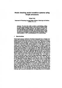
We use Transition Diagram (TD) to model a concurrent system. Formally, a TD is a triple G = (Q, X, E) such that Q denotes a set of nodes, X is a set of variables, and E is a set of transitions which are quadruples of the form hq, C, Λ, q 0 i where q, q 0 ∈ Q, C is a condition involving the variables in X and Λ is a set of assignments of the form x := ρ where x ∈ X and ρ is an expression involving the variables in X. For a transition hq, C, Λ, q 0 i, we call C the condition part or guard of the transition and Λ the action part of the transition and we require that Λ contains at most one assignment for each variable. For any node q of G, we let guards(q) denote the set of guards of transitions from the node q. We also let guards(G) denote the set of guards of all transitions of G. An evaluation h of a set of variables X is a function that assigns type-consistent values to each variable in X. A state of a TD G = (Q, X, E) is a pair (q, h) where q ∈ Q and h is an evaluation of X. We say that a transition e = (q1 , C, Λ, q2 ) is enabled in the state (q, h) if q = q1 and the condition C is satisfied by h, i.e., the values of the variables given by h satisfy C. We say that a state (q 0 , h0 ) is obtained from (q, h) by executing the transition e if e is enabled in (q, h), q 0 = q2 and the following property is satisfied: for each variable x ∈ X, if there is an assignment of the form x := ρ in Λ then h0 (x) = h(ρ), otherwise h0 (x) = h(x). A path in G from node q to node r is a sequence of transitions starting with a transition from q and ending with a transition leading to r such that each successive transition starts from the node where the preceding transition ends. Let π = e0 , e1 , ..., em−1 be a path in G from node q and let s0 = (q, h0 ) be a state. We say that π is feasible from s0 if there exists a sequence of states s1 , ..., sm such that for each i, 0 ≤ i < m, the transition ei is enabled in si and state si+1 is obtained by executing ei in the state si . In this case, i.e., when π is feasible from s0 , we say that sm is the state obtained by executing the path π from s0 . The left part of figure 1 shows a TD with node set {0, 1, 2}, variable set {a, b, x, y} and transition set {t1 , t2 , t3 , t4 }. Notice that the transition t1 and t2 both have empty guards meaning that they are always enabled. It is easy to see that the reachability graph from an initial state may be infinite since x, y can grow arbitrarily large.

(1,

t3 : a≤y → y++

1

0

s1 (0,

t1 : a:=x; x++

t2 : b:=x; x++

0 0 0 0 a b x+1 y )

0 0 0 0 a b x y)

s0

s2

2

t4 : b≤y → x:=0; y:=0

s3

(2,

0 0 0 0 a b x+1 y )

Fig. 1. Example of a TD and its reduced symbolic state graph

Commutativity Requirement

(0,

0 0 0 0 a b x+1 y+1 )

In this paper, we consider the TDs whose action parts only have assignments of the following forms: x := c where c is a constant, or x := ψ(x), or x := y where y is another variable of the same type as x. We require all functions that are applied to variables of the same type to be commutative. We call such TDs as simple TDs. In section 8.2, we show how the commutativity requirement can be further relaxed. 3.2

Kripke Structures, Bi-simulation, etc.

A labeled Kripke structure H over a set of atomic propositions AP and over a set of labels Σ is a triple (S, R, L) where S is a set of states, R ⊆ S × Σ × S and L : S → 2AP associates each state with a set of atomic propositions. The Kripke structure H is said to be deterministic if for every s ∈ S and every α ∈ Σ there exists at most one s0 ∈ S such that (s, α, s0 ) ∈ R. For the Kripke structure H = (S, R, L), an execution σ is an infinite sequence s0 , e0 , s1 , e1 , ..., si , ei , ... of alternating states and labels in Σ such that for each i ≥ 0, (si , ei , si+1 ) ∈ R. A finite execution is a finite sequence of the above type ending in a label in Σ. Corresponding to the execution σ that is finite or infinite, let trace(σ) denote the sequence L(s0 ), e0 , ..., L(si ), ei , .... A finite trace from state s is the sequence trace(σ) corresponding to a finite execution from s. The length of a finite trace is the number of transitions in it. For any integer k > 0, let F inite T racesk (H, s) denote the set of finite traces of length k from s. Let H = (S, R, L) and H 0 = (S 0 , R0 , L0 ) be two structures over the same set of atomic propositions AP and the same set Σ of labels. A relation B ⊆ S × S 0 is a bi-simulation between H and H 0 iff for all s ∈ S and s0 ∈ S 0 , if (s, s0 ) ∈ B, then L(s) = L(s0 ) and the following conditions hold: (a) for every (s, α, s1 ) ∈ R, there exists a state s01 ∈ S 0 such that (s0 , α, s01 ) ∈ R0 and (s1 , s01 ) ∈ B; (b) similarly, for every (s0 , α, s01 ) ∈ R0 , there exists a state s1 ∈ S such that (s, α, s1 ) ∈ R and (s1 , s01 ) ∈ B. Let G = (Q, X, E) be a TD and Reach(G, u) = (S, R, L) denote the Kripke structure over the set of atomic propositions AP and the set of labels E defined as follows: S is the set of reachable states obtained by executing the TD G from u; R is the set of triples (s, e, s0 ) such that the transition e ∈ E is enabled in state s and s0 is obtained by executing e in state s; for any s ∈ S, L(s) is the set of atomic propositions in AP that are satisfied in s. It is not difficult to see that Reach(G, u) is a deterministic structure. Let B be a bi-simulation relation from Reach(G, u) to itself. Instead of constructing Reach(G, u), we can construct a smaller structure using the relation B. We incrementally construct the structure by executing G starting from u. Whenever we get a state w by executing a transition from an already reached state v, we check if there exists an already reached state w 0 such that (w, w0 ) or (w0 , w) is in B; if so, we simply add an edge to w 0 or else we include w into the set of reached states and add an edge to w. This procedure is carried until no more new nosed can be added to the set of reached states. We call the resulting structure as the bi-simulation reduction of Reach(G, u) with respect to B. This reduction has the property that no two states in it are related by B. The number of states in this reduction may not be unique and may depend on the the order of execution of the enabled transitions. However, if B is an equivalence relation then the number of states in the reduction is unique and equals the number of equivalence classes of S with respect to B. Let G be a TD that captures the behavior of a concurrent program. The Kripke structure Reach(G, u) is deterministic. An infinite execution σ is said to be weakly fair if every process which is enabled continuously from a certain point in σ is executed infinitely often. Let F air traces(s) denote the set of all trace(σ) where σ is an infinite weakly fair execution s. For any bi-simulation B from Reach(G, u) to itself, it is easy to show that for every (s, t) ∈ B, F air traces(s) = F air traces(t). This condition holds many other fairness conditions such as strong fairness, etc.

We use the temporal logic CTL* to specify properties of Reach(G, u). Each atomic proposition in the formulas is a predicate involving variables in X or the special variable lc which refers to the nodes of G. We let AP be the set of predicates that appear in the temporal formula that we want to check. For any formula or predicate p, we let var(p) denote the set of variables appearing in it. If K is a reduction of Reach(G, u) with respect to a bi-simulation relation then a state which is present in both Reach(G, u) and K satisfies the same set of CTL* formulas in both structures even if we restrict the paths to fair paths. Also, any two states in Reach(G, u) that are bi-similar to each other satisfy the same set of CTL* formulas. We also use the following notation. If Φ represents an expression, then Φ{β/α} is the expression obtained from Φ by substituting β for α. 3.3

Symbolic State graph

Let G = (Q, X, E) be a TD, u = (q0 , h0 ) be the initial state of G and AP be the set of predicates that appear in the temporal formula to be checked. We execute G symbolically starting with u, to obtain a structure Sym Reach(G, u) = (S 0 , R0 , L0 ). We call the structure Sym Reach(G, u) as the symbolic graph and the states of S 0 symbolic states since the variables are represented by expressions. (It should be noted that our use of the term symbolic state is different from the traditional use where it is meant to be some representation for sets of actual states). Each state s in S 0 is a triple of the form (s.lc, s.val, s.exp) where s.lc ∈ Q, s.val is an evaluation of the variables in X and s.exp is a function that assigns each variable x an expression which involves only the variable x. Intuitively, s.lc denotes the node in Q where the control is, s.val(x) denotes the latest constant assigned to x and s.exp(x) denotes the composition of functions that were applied to x since then. We associate each symbolic state s with a state act state(s) of G defined as follows: act state(s) = (q, h) where q = s.lc and h(x) = s.exp(x){s.val(x)/x} for each x ∈ X; that is the value of a variable x is obtained by evaluating s.exp(x) after substituting s.val(x) for x in the expression. We say that a transition e is enabled in a symbolic state s if it is enabled in the corresponding actual state, i.e., it is enabled in act state(s). The successor states of a symbolic state s are the states obtained by enabled transitions in s. Assume that e = (q, C, Λ, q 0 ) is enabled in s. The new symbolic state s0 obtained by executing e from s is defined as follows: s0 .lc = q 0 and for each variable x, if there is no assignment to x in Λ then s0 .val(x) = s.val(x) and s0 .exp(x) = s.exp(x). If there is an assignment of the form x := c where c is a constant then s 0 .val(x) = c and s0 .exp(x) = x. If there is an assignment of the form x := ψ(x) in Λ then s0 .val(x) = s.val(x) and s0 .exp(x) = ψ(s.exp(x)); that is the value remains unchanged and the new expression is obtained by applying the function ψ to the old expression. If there is an assignment of the form x := y in Λ then s0 .val(x) = s.val(y) and s0 .exp(x) = s.exp(y){x/y}; that is the value of s.val(y) is copied and the expression of y in s is also copied after replacing every y by x in the expression. If s 0 is obtained by executing an enabled transition e from a state s in S 0 , then s0 is a state in S 0 and (s, e, s0 ) ∈ R0 . Also for any s ∈ S 0 , L0 (s) = L(act state(s)). Consider the TD given in the left part of figure 1 with initial value a = b = x = y = 0. We represent each variable v ∈ X as a pair (v.val, v.exp). The actual value of v is v.exp{v.val/v}. For figure 1, the initial state s0 is (0, a0 0b x0 y0 ), where the first 0 denotes the node, the vectors (0, 0, 0, 0) and (a, b, x, y) represent the functions s0 .val and s0 .exp respectively. In s0 , transition t1 and t2 are enabled. Suppose we execute t1 from s0 and get state s1 . The node in s1 is 1. For variable a, since x is assigned to it, we copy x.val and x.exp to a.val and a.exp respectively. For variable x, which is updated by a function of itself, we keep x.val as before and change x.exp from x to x + 1 according to the updating function. Since 0 0 there is no assignment to b and y in t1 , their val and exp remain unchanged. So, s1 is (1, a0 0b x+1 y ). We

know t3 is enabled in s1 since the actual values of a, y satisfy the guard. We execute t3 from s1 and get 0 0 s2 = (0, a0 0b x+1 y+1 ) similarly. Similarly, executing t2 from s0 we get s3 . Executing t4 from s3 we get s0 ; notice that since x is assigned 0, in the successor state s0 we have s.val(x) = 0 and s.exp(x) = x and same holds for variable y. Lemma 1 Let G be a TD, u be a state of G. Then the binary relation {(act state(s), s) : s is a symbolic state in Sym Reach(G, u)} is a bi-simulation between Reach(G, u) and Sym Reach(G, u).

4 4.1

Our method Intuitive Description

Let G = (Q, X, E) be a TD. Recall that AP is the set of predicates appearing in the temporal formula. We motivate our definition of the bi-simulation relation and give an intuitive explanation for the commutativity requirement. For ease of explanation, assume that all the assignments in the transitions of G are of the form x := ψ(x). Also assume that all the predicates in guards(G) ∪ AP have at most one variable. It is not difficult to see that any two states s = (q, h) and t = (q, h0 ) satisfying the following conditions are bisimilar in Reach(G, u): (i) for every path π from node q, π is feasible in s iff it is feasible from t; (ii) for every path π from node q to any node r such that π is feasible from s, if s0 , t0 are the states obtained by executing π from s, t respectively then s0 , t0 satisfy the same predicates in guards(r) ∪ AP . For any path π in G and variable x ∈ X, let Fπ,x denote the composition of the functions that update the variable x in the path π where the composition is taken in the order they appear on the path. Using the above observation, it can be seen that the following relation U over the states of Reach(G, u) is a bi-simulation. U is the set of all pairs (s, t) of states where s = (q, h), t = (q, h0 ) for some q ∈ Q and some evaluations h, h0 such that the following condition is satisfied: for every node r and for every path π from q to r in G, and for every predicate p(x) ∈ guards(r) ∪ AP , the truth values p(x){F π,x (h(x))/x} and p(x){Fπ,x (h0 (x))/x} are the same. Analogous to the relation U , we can define a relation V over the states of the symbolic graph Sym Reach(G, u) as follows. V is the set of all pairs (v, w) of symbolic states where v.lc = w.lc = q for some q ∈ Q, v.val(x) = w.val(x) = c for some constant c and for every node r to which there is a path in G from node q, and for every predicate p(x) ∈ guards(r) ∪ AP the following condition (A) is satisfied: (A) for every path π from q to r in G, the truth values p(x){Fπ,x (ρ1 (c))/x} and p(x){Fπ,x (ρ2 (c))/x} are the same where ρ1 (x), ρ2 (x) are the expressions v.exp(x), w.exp(x) respectively. Note that ρ1 (c) is the value of ρ1 (x) when c is substituted for x. It is not difficult to see that V is also a bi-simulation over Sym Reach(G, u). Due to the commutativity requirement on the functions that update variables, we can see that Fπ,x (ρ1 (c)) = ρ1 (Fπ,x (c)) and a similar equality holds for the state w. As a consequence, condition (A) can be rewritten as follows: (B) for every path π from q to r in G, the truth values p(x){ρ1 (Fπ,x (c))/x} and p(x){ρ2 (Fπ,x (c))/x} are equal. Now we see that condition (B) is automatically satisfied if the two predicates p(x){ρ1 (x)/x} and p(x){ρ2 (x)/x} are equivalent ( this is seen by substituting the value Fπ,x (c) for x in these two predicates). As a consequence we can replace condition (A) by condition (C) which requires the equivalence of the above two predicates. Checking condition (A) requires considering every path from q to r which is not needed for checking (C). (Using (C) in place of (A) might give us a smaller relation ρ1 ; this disadvantage is minimized using the extensions of section 8.1). The above argument holds even if we have predicates with more than one free variable in guards(G) ∪ AP . However, if we have other types of assignments to variables then we need to rename some of the variables to obtain the predicates whose equivalence needs to be checked. This is done by computing a set of predicate templates with respect to each node in G.

4.2

Predicate Templates

To define the bi-simulation, we associate a set of predicate templates, denoted ptemplates(q), with each node q in the TD. Intuitively, ptemplates(q) is the set of pairs of predicates and renaming functions on their variables; roughly speaking, our bi-simulation condition requires that the predicates, obtained by renaming the variables and substituting them by the corresponding expressions in two symbolic states, should be equivalent. Formally, a predicate template is a pair (p, f ) where p is a predicate and f , called renaming function, is a total function from var(p) to X ∪ {∗}. First we need the following definition. Let π be a path in G. Each such path denotes a possible execution in G. With respect to π, we define a function dependsπ from X to X ∪ {∗}. Intuitively, if dependsπ (x) is a variable, say y, then this denotes that the value of x at the end of the execution of π depends on the value of y at the beginning of this execution; otherwise, i.e., depends π (x) = ∗, the value of x at the end of π does not depend on the value of any variable at the beginning of π; for example, this happens if x is assigned a constant some where along π. We define dependsπ inductively on the length of π. If π is a single transition hq, C, Λ, q 0 i then dependsπ (x) is given as follows: if Λ has the assignment x := y then dependsπ (x) = y; if Λ has no assignment to x or has an assignment of the form x := ψ(x) then dependsπ (x) = x; when x is assigned a constant, dependsπ (x) = ∗. If π is the path consisting of π1 followed by π2 then dependsπ is defined as follows: for each x ∈ X, if dependsπ2 (x) is a variable then dependsπ (x) = dependsπ1 (dependsπ2 (x)), otherwise dependsπ (x) = ∗. For the TD given in figure 1 and the path π given by the single transition from node 0 to 1, we see that depends π (a) = x. For a node q, ptemplates(q) = {(p, dependsπ ) : π is a path from node q to some node r and p ∈ guards(r) ∪ AP }. Although the number of paths from q can be infinite, the number of functions dependsπ and hence ptemplates(q) is a bounded set. We can compute ptemplates(q) without examining all the paths from q as follows. For a template (p, f ) and a set of assignments Λ, let (p, f )Λ be the template (p, f 0 ) where f 0 is given as follows: (note that (p, f 0 ) is different from the the weakest precondition of p with respect to Λ) – if f (x) = ∗, then f 0 (x) = ∗. – if f (x) = y where y ∈ X, then if the action part Λ has • no assignment for y or an assignment of the form y := ψ(y), then f 0 (x) = y = f (x). • an assignment of the form y := z, then f 0 (x) = z. • an assignment of the form y := c where c is a constant, then f 0 (x) = ∗. Let fid be the identity function. For each node q ∈ Q, the set ptemplates(q) is the least fix point solution for the variables temp(q) in the following set of equations: temp(q) ={(p, fid )|p ∈ AP ∨ p ∈ guards(q)} ∪ {(p, f )Λ |(p, f ) ∈ temp(q 0 ) ∧ ∃(q, C, Λ, q 0 ) ∈ E} Consider the system given in figure 1. Suppose we want to check the formula ∀ (x ≥ y). Let p 0 denote x ≥ y, p1 denote a ≤ y, p2 denote b ≤ y. Template (p0 , fid ) will appear in templates of each location since it is in AP . (p1 , fid ) will appear in ptemplates(1) since p1 is in guards(1). In the remainder of our description, we will also represent a predicate template (p, f ) where f maps v1 , v2 to z1 , z2 respectively by the tuple (p, v1 : z1 , v2 : z2 ). Suppose t is a transition, let Λt denote the action part of t. By definition, (p1 , fid )Λt1 will appear in ptemplate(0). Since Λt1 contains the assignments a := x and x := x + 1, the template (p1 , fid )Λt1 is given by (p1 , a : x, y : y). Using transition t4 , we see that the template (p0 , x : ∗, y : ∗) is in

ptemplates(2); note that in this template both the variables are mapped to ∗ since both these variables are assigned constant values in t4 . By doing this, eventually, we will have ptemplates(1) ={(p0 , fid ), (p1 , fid ), {(p1 , a : x, y : y), (p2 , b : x, y : y)} We have only given the templates associated with node 1 and even from this we omitted the templates whose renaming function maps all the variables to ∗. From the above definition, we see that ptemplates(q) contains all the templates in {(p, fid )|p ∈ AP ∪ guards(q)}. We can use standard fix point algorithm to compute the set ptemplates(q) for each q ∈ Q. It is easy to see that the algorithm terminates since the total number of predicate templates is bounded. Let Nn , Nt , Nv be the number of nodes in G, number of transitions in G and the number of variables respectively. Similarly let Np and Na respectively be the number of predicates in guards(G) ∪ AP and the maximum number of variables appearing in any predicate. Since the maximum number of renaming functions is (Nv + 1)Na , we see that the maximum number of predicate templates is Np · (Nv + 1)Na . Thus the number of the outer iterations of the fix point computations is at most Nn · Np · (Nv + 1)Na . The time complexity of the algorithm is O(Nn · Np · Nt · (Nv + 1)Na ). Thus we see that the number of predicates is exponential in the number of variables that can appear in a predicate. In most cases we have unary or binary predicates and hence the complexity will not be a problem. Also this worst case complexity occurs when every variable is assigned to every other variable directly or indirectly. We believe that this is a rare case. 4.3

Definition of the bi-simulation relation

Now we define the instantiation of a predicate template in a symbolic state. Suppose s is a state of the symbolic state graph Sym Reach(G, u), (p, f ) is a predicate template and x1 , x2 , · · · , xn are variables appearing in p. Let p0 be the predicate obtained by replacing every occurrence of the variable xi (for 1 ≤ i ≤ n), for those xi such that f (xi ) 6= ∗, by the expression s.exp(yi ){xi /yi } where yi is the variable f (xi ). Note that the variables xi for which f (xi ) = ∗ are not replaced. We define (p, f )[s] to be p0 as given above. For the system given in figure 1, it is easy to see that for the state s1 , (p1 , a : x, y : y)[s1 ] is a + 1 ≤ y. Note that for those templates whose renaming function maps all the variables to ∗, the instantiation of them in any two symbolic states will be identical and thus they are trivially equivalent. We can just ignore such templates. Definition 1. Define relation ∼0 as follows: For any two states s and t, s ∼0 t iff s.lc = t.lc, s.val = t.val and for each (p, f ) ∈ ptemplates(s.lc), (p, f )[s] ≡ (p, f )[t] is a valid formula. Theorem 1. ∼0 is a bi-simulation on the symbolic state graph Sym Reach(G, u). It is possible that two symbolic states s, t correspond to the same actual state but (s, t) ∈∼ / 0 . To overcome this problem, we consider the relation ∼equal = {(s, t) : s, t are symbolic states and act state(s) = act state(t)}. Clearly, ∼equal is a bi-simulation on Sym Reach(G, u). Given symbolic states s, t checking if (s, t) ∈∼equal is simple. We simply compute act state(s) and act state(t) and check if they are equal. Now, we consider the relation ∼0 ∪ ∼equal . It is well known that the union of bi-simulation relations is also a bi-simulation. ¿From this, we see that ∼0 ∪ ∼equal is a bi-simulation on Sym Reach(G, u). The

reduction of Sym Reach(G, u) with respect to the bi-simulation ∼0 ∪ ∼equal has at most as many states as the number of states in Reach(G, u). Checking if s ∼0 t requires checking equivalence of predicates (p, f )[s] and (p, f )[t] for each template (p, f ) ∈ ptemplates(s.lc). Section 8.1 in the appendix also introduces a bi-simulation ∼ 00 which is obtained by constraining the universal quantifiers over variables in the above predicate equivalence. These constraints on the quantifiers are generated by performing a static analysis of the TD. Subsection 8.1 in the appendix discusses how this equivalence check can be done efficiently for the integer domains. It also shows how the regular reachability graph. Reach(G, u), instead of Sym Reach(G, u), can be used to define a bi-simulations ≈0 , ≈00 and use them for model checking.

5

Bi-simulation Relations with respect to the Paths in the TD

In section 4, we defined the bi-simulation relation ∼0 . Two symbolic states s, t are related by this relation, if s.lc = t.lc and for every node r and for every p ∈ guards(r)∪AP and for every path π from s.lc to r, the two predicates (p, dependsπ )[s] and (p, dependsπ )[t] are equivalent (note that (p, dependsπ ) is a template in ptemplates(s.lc)). If none of the guards of transitions entering r is satisfiable then we don’t need to require the equivalence of the above two predicates since r is never reached. We define a bi-simulation relation ∼1 in which we relax the condition equivalence condition. Suppose e is a transition entering node r, then in the definition of ∼1 , we require the equivalence of (p, dependsπ )[s] and (p, dependsπ )[t] only for those cases when the transition e is enabled with respect to both s and t. Such a requirement will be made with respect to every transition entering r. This notion of relaxing the requirement can be generalized to paths of length k entering node r leading to bi-simulation relations ∼ k for each k > 0. We describe this below. First, we need the following definitions. Let π be a path in G and p be any predicate. We define the weakest precondition of p with respect to π, denoted by W P (π, p), inductively on the length of π as follows. If π is of length zero, i.e., π is an empty path then W P (π, p) = p. If π is a single transition given by (r, C, Λ, r0 ), where Λ is the set of assignments x1 := ρ1 , ..., xk := ρk , then W P (π, p) is the predicate p{ρ1 /x1 , ..., ρk /xk }. If π has more than one transition and consists of the path π 0 followed by the single transition e then W P (π, p) = W P (π 0 , W P (e, p)). The following lemma is proved by a simple induction on the length of π. (It is to be noted that our definition of the weakest precondition is slightly different from the traditional one; for example, the traditional weakest precondition is C ⊃ W P (π, p) for the case when π is a single transition with guard C). Lemma 2 If path π of G is feasible from state s, and t is the state obtained by executing π from s, then t satisfies p iff s satisfies W P (π, p).  Let π = e0 , e1 , ..., ek−1 be a path in G where, for 0 ≤ i < k, Ci is the guard of the transition ei . For each i, 0 < i ≤ k, let π(i) denote the prefix of π consisting of the first i transitions, i.e., the prefix up V to ei−1 . Define Cond(π) to be the predicate C0 ∧ 0 0, ∼k is a bi-simulation relation.  The bi-simulation relation ∼k is defined using paths of length k. We can consider the relation ∼0 defined in section 4 as ∼k for k = 0; in this case, we consider an empty path as a path of length zero. The following theorem states that ∼k is contained in ∼k+1 for each k ≥ 0 and that for for every k there exists a TD in which this containment is strict. The proof of the theorem is given in the appendix. Theorem 3. (1) For every k ≥ 0, every TD G, and for every set AP of atomic predicates, ∼ k ⊆∼k+1 . (2) For every k ≥ 0, there exists a TD G and a set of atomic predicates AP for which the above containment is strict, i.e. ∼k ⊂∼k+1 . The set extended templates(q, k) for any node q and for any k > 0 can be computed using a fix point computation just like the computation of ptemplates(q). An efficient way to check condition (b) in the definition of ∼k , i.e., to check F inite T racesk (Reach(G, u), s) = F inite T racesk (Reach(G, u), s), is as follows. First check that s and t satisfy the same predicates from AP . For every transition e enabled from s, check that e is also enabled from t and vice versa; further, if s0 , t0 are the states obtained by executing e from s, t respectively, then inductively check that F inite T races k−1 (Reach(G, u), s0 ) = F inite T racesk−1 (Reach(G, u), t0 ). This method works because Reach(G, u) is a deterministic structure. It is to be noted that for any i < j, checking if (s, t) ∈∼j is going to be more expensive than checking if (s, t) ∈∼i . This is because checking condition (c) in the definition of ∼i is less expensive since it requires checking equivalence of fewer formulas since extended templates(q, i) is a smaller set than extended templates(q, i). Similarly, checking condition (b) is less expensive for ∼ i since the number of traces of length i less than the number of traces of length j. However, the bi-simulation reduction with respect to ∼j will be smaller. Thus there is a trade off. We believe that, in general, it is practical to use ∼i for small values of i such as i = 0, 1, etc. As in the section 4, for each i > 0, we can use the bi-simulation ∼i ∪ ∼equal on the Sym Reach(G, u) to get a smaller bi-simulation reduction. Section 8.1 in the appendix defines bi-simulations ∼0k analogous to ∼00 by constraining the domain of universal quantifiers in the predicate equivalences. Analogous to ≈ 0 and ≈00 , it also defines bi-simulations ≈k and ≈0k for integer domains over Reach(G, u) for each k > 0.

The appendix discusses and gives an example TD, shown in figure 2, for which the bi-simulation ≈ 1 gives more reduction than ≈0 .

6

Experimental Results

We implemented the method given in the paper for checking invariance properties. This implementation uses the reduction with respect to the bi-simulation ∼0 . Our implementation takes a concurrent program given as a transition system T . The syntax of the input language is similar to that of SMC [17]. The input variables can be either binary variables or integer variables. The implementation has two parts. The first part reads the description of T and converts it in to a TD G by executing the finite state part of it. All the parts in the conditions and actions that refer to integer variables in the transitions of T are transferred to guards and actions in the transitions of G. The second part of the implementation constructs the bi-simulation reduction of G given in section 4 and checks the invariance property on the fly. We tested our implementation for a variety of examples. Our implementation terminated in all cases excepting for the example of an unbounded queue implementation. In those cases where it terminated, it gave the correct answer. One of our examples is the sliding window protocol with bounded channel. It is an infinite state system due to the sequence numbers. This protocol has a sender and receiver process communicating over a channel. The sender transmits messages tagged with sequence numbers and the receiver sends acknowledgments (also tagged with sequence numbers) after receiving a message. We checked the safety property that every message value received by the receiver was earlier transmitted by the sender. We tested this protocol with a bounded channel under different assumptions. The results are given in Table 2. The table shows the window sizes, the time in seconds, the number of states and edges in the reduced graph and the environment for which the protocol is supposed to work (here “duplicates” means the channel can duplicate messages, “lost” means the channel can lose messages).

Problem Instance Ticket algorithm ProducerConsumer size of buffer 30 100 Circular Queue size of queue 10

30

Property ∀(¬(pc1 = C1 ∧ pc2 = C2 )) Property

t in sec # of states 0 9 t in sec # of states

∀(0 ≤ p1 + p2 − (c1 + c2 ) ≤ s) ∀(0 ≤ p1 + p2 − (c1 + c2 ) ≤ s) Property

0.01 31 0.09 101 t in sec # of states

∀(h ≤ s ∧ t ≤ s) ∀(t ≥ h → p − c = t − h) ∀(t ≤ h → p − c = s − (h − t) + 1) ∀(0 ≤ p − c ≤ s) ∀(h ≤ s ∧ t ≤ s) ∀(t ≥ h → p − c = t − h) ∀(t ≤ h → p − c = s − (h − t) + 1) ∀(0 ≤ p − c ≤ s) Table 1. Summary of the tests.

0.24 0.12 0.12 0.15 16.4 2.8 2.7 3.2

121 121 121 121 961 961 961 961

We also tested with three other examples taken from [6]. These are the Ticket algorithm for mutual exclusion, Producer-Consumer algorithm and Circular queue implementation. The detailed descriptions of these examples can be found in [6]. All these examples use integer variables as well as binary variables. The ticket algorithm is an algorithm similar to the bakery algorithm. We checked the mutual exclusion property for this algorithm. The Producer-Consumer algorithm consists of two producer and two consumer processes. The producer processes generate messages and place them in a bounded buffer which are retrieved by the consumer processes. In this algorithm, the actual content of the buffer is not modeled. The algorithm uses some binary variables, four integer variables p1 , p2 , c1 , c2 and a parameter s denoting the size of the buffer. Here p1 , p2 denote the total number of messages generated by each of the producers respectively; similarly, c1 , c2 denote the number of messages consumed by the consumers. The circular queue example has the bounded variables h, t which are indexes into a finite array, positive integer variables p, c and a parameter s that denotes the size of the buffer. Here p, c respectively denote the number of messages that are enqueued and dequeued since the beginning. In all these examples, our method terminated and the results are shown in table 1. Time in the table is the time used to get the reduced symbolic state graph. Checking the property does not take that much time. We have also implemented the method using the relation ∼1 . We run it on examples such as the one given in figure 2 and get a smaller bi-simulation reduction. More realistic examples need to be further examined. Sender Window Receiver Window t[s] # of states # of edges Environment 1 1 0.016 47 164 duplicate, lost 1 2 0.203 447 1076 duplicate 1 2 0.296 509 1731 duplicate, lost 2 1 0.860 1167 3832 duplicate 2 2 11.515 4555 11272 duplicate Table 2. Experiment on sliding window protocol.

7

Conclusion

In this paper we gave methods for model checking of concurrent programs modeled by simple Transition Diagrams. We have given a chain of non-decreasing bi-simulation relations, ∼i for each i ≥ 0, on these TDs. They are defined by using predicate templates and extended predicate templates that can be computed by performing a static analysis of the TD. Recall that ∼i is defined by using templates with respect paths of length i in the TD. Each of these bi-simulations require that the two related states be indistinguishable with respect to the corresponding templates. All these relations can be used to compute a reduced graph for model checking. We have also given how some of these bi-simulation conditions can be checked efficiently for certain types of programs. We have also shown how they can be used to show the decidability of the reachability problem of some simple hybrid automata when the time domain is discrete. We have also presented variants of the above approaches. We have implemented the model checking method using the bi-simulations ∼0 , ∼1 . We have given experimental results showing their effectiveness. To the best our knowledge, this is the first time such a comprehensive analysis of simple TDs has been done and the various types of bi-simulations have been defined and used.

Further work is needed on relaxing some of the assumptions such as the commutativity and also on weakening the equivalence condition. Further investigation is also needed on identifying classes of programs to which this approach can be applied.

References 1. R. Alur and D. L. Dill. A theory of timed automata. Theoretical Computer Science, 126(2):183–235, 1994. 2. T. Ball and S. K. Rajmani. The slam toolkit. In CAV2001, 2001. 3. T. Ball and S. K. Rajmani. The slam project: Debugging system software via static analysis. In ACM Symposium on Principles of Progarmming Languages, 2002. 4. G. Behrmann, E. Bouyer, Patricia Fleury, and K. G. Larsen. Static guard analysis in timed automata verification. In TACAS, pages 254–270, 2003. 5. B. Boigelot and P. Wolper. Symbolic verification with periodic sets. In D. L. Dill, editor, CAV94, Stanford, California, USA, Proceedings, volume 818 of Lecture Notes in Computer Science, pages 55–67. Springer, 1994. 6. T. Bultan, R. Gerber, and W. Pugh. Model-checking concurrent systems with unbounded integer variables: symbolic representations, approximations, and experimental results. ACM Trans. Program. Lang. Syst., 21(4):747–789, 1999. 7. E. M. Clarke, O. Grumberg, S. Jha, Y. Lu, and H. Veith. Counter-example guided abstraction refinement. In CAV 2000, Chicago, IL, USA, July 15-19, 2000, Proceedings, volume 1855 of Lecture Notes in Computer Science. Springer, 2000. 8. P. Godefroid. Partial-order methods for the verification of concurrent systems: an approach to the stateexplosion problem, volume 1032. Springer-Verlag Inc., New York, NY, USA, 1996. 9. H.Saidi and N. Shankar. Abstract and model check while you prove. In N. Halbwachs and D. Peled, editors, CAV99, Trento, Italy,Proceedings, volume 1633 of Lecture Notes in Computer Science, pages 443–454. Springer, 1999. 10. D. Lee and M. Yannakakis. Online minimization of transition systems (extended abstract). In Proceedings of the twenty-fourth annual ACM symposium on Theory of computing, pages 264–274. ACM Press, 1992. 11. Z. Manna and A. Pnueli. The Temporal Logic of Reactive and Concurrent Systems: Specification. SpringerVerlag, Berlin, Jan. 1992. 12. K. S. Namjoshi and R. P. Kurshan. Syntactic program transformations for automatic abstraction. In CAV2000, pages 435–449, 2000. 13. D. Peled. All from one, one for all, on model-checking using representatives. In C. Courcoubetis, editor, CAV 93, Elounda, Greece, Proceedings, volume 697 of Lecture Notes in Computer Science, pages 409–423. Springer, 1993. 14. C. C. R. Alur and et al. The algorithmic analysis of hybrid systems. Theoretical Computer Science, 138:3–34, 1995. 15. T. H. R. Alur, C. Courcubetis and P. H. Ho. Hybrid automata: An algorithmic approach to the specification and verification of hybrid systems. In Hybrid Systems, volume 736 of Lecture Notes in Computer Science, pages 209–229, 1993. 16. S. Graf and H. Saidi. Construction of abstract state graphs with PVS. In O. Grumberg, editor, CAV97, volume 1254, pages 72–83. Springer Verlag, 1997. 17. A. P. Sistla, V. Gyuris, and E. A. Emerson. Smc: A symmetry based model checker for safety and liveness properties. ACM Transactions on Software Engineering Methodologies, 9(2):133–166, 2000. 18. A. P. T. A. Henzinger, P. W. Kopke and P. Varaiya. What’s decidable about hybrid automata? Journal of Computer and System Sciences, 57:94–124, 1998. 19. J. S. X. Nicollin, A. Olivero and S. Yovine. An approach to description and analysis of hybrid systems. In Hybrid Systems, volume 736 of Lecture Notes in Computer Science, pages 149–178, 1993. 20. J. S. Y. Kesten, A. Pnueli and S. Yovine. Integration graphs: A class of decidable hybrid systems. In Hybrid systems, volume 736 of Lecture Notes in Computer Science, pages 179–208. Springer-Verlag, 1993.

8 8.1

Appendix Extensions and Special cases

Using static analysis to constrain the quantifiers’ range In subsection 4.3 we have defined a bi-simulation relation ∼0 on the states of Sym Reach(G, u). Under this definition, s ∼0 t if s.lc = t.lc, s.val = t.val and for each template (p, f ) ∈ ptemplates(s.lc), (p, f )[s] ≡ (p, f )[t] is valid. Note that var(p) is also the set of variables that appear free in (p, f )[s] and (p, f )[t]. It should also be noted that there is an implicit universal quantification on the variables in var(p) in the equivalence (p, f )[s] ≡ (p, f )[t] when we assert its validity. This universal quantification can be restricted to range over a smaller set of values in some cases. By this change, we get another relation which is also a bi-simulation that is larger than ∼0 . Consider any state s in Sym Reach(G, u). Let (p, f ) be any predicate template in ptemplates(s.lc) such that p ∈ guards(G) ∪ AP . Let {x1 , ..., xn } be all the variables in var(p) and Qp ⊆ Q be as defined below: if p ∈ AP then Qp = Q, otherwise Qp is the set of all nodes q in G such that p ∈ guards(q). Let G0 be the TD obtained from G by replacing all guards in its transitions by the constant predicate T rue. Now let Tp,s be the set of n-tuples (c1 , ..., cn ) respectively denoting the values of variables x1 , ..., xn in some state (q, h), where q ∈ Qp , that is reachable from the state (s.lc, s.val) in the Reach(G0 , u). Essentially, Tp,s is the set of all tuples of values for the variables x1 , ..., xn when the control is at some node in Qp when the T D G0 is executed starting from the state (s.lc, s.val). Let gp,s be a formula with free variables x1 , ..., xn that defines any super set of Tp,s , i.e., every tuple in Tp,s satisfies the constraint given by gp,s . Essentially, gp,s defines a constraint on the values of the variables when the control is at some node in Qp . Let ∼00 be the set of (s, t) such that s, t are symbolic states, s.lc = t.lc, s.val = t.val, for all (p, f ) ∈ ptemplates(s.lc) the formula gp,s ⊃ ((p, f )[s] ≡ (p, f )[t]) is valid. Thus we see that the quantifiers over x1 , ..., xn are restricted to the tuples that satisfy gp,s , i.e., the tuples in Tp,s . Observe that Tp,s = Tp,t ; thus it does not matter whether we use s or t for obtaining these sets and the formulas g p,s . It should be easy to see that ∼00 ⊇ ∼0 . The following theorem can be proved on the same lines as theorem 1. Theorem 4. ∼00 is a bi-simulation on symbolic state graph Sym Reach(G, u).  We can also define relations ∼0i , for each i > 0, by performing static analysis and by constraining the domain of the universal quantifiers over the free variables in the conditional predicate equivalences of ∼ i for each i > 0. Formally, ∼0i is the set of symbolic state pairs (s, t) such that s.lc = t.lc and the following is satisfied: for each triple (p1 , p2 , f ) ∈ extended templates(s.lc, i), we require that (gp,s ∧ (p1 , f )[s] ∧ (p1 , f )[t]) ⊃ ((p2 , f )[s] ≡ (p2 , f )[t]) be a valid formula where gp,s is as defined above. It is also not to difficult to see, using theorem 2, that each ∼0i (for i > 0) is a bi-simulation. In the above definitions, we see that the formulas gp,s depend on p, s.lc and s.val. Note that the set of possible values of s.val can be determined from static analysis of G. Essentially, for any variable x, s.val(x) is a constant that is assigned to x in the action part of some transition. Since G 0 has only the guards T rue in all transitions, it is not difficult to see that the set of tuples Tp,s or the formulas gp,s can be computed by performing a static analysis of G. The number of values for s.val can be exponential. Many times we can get a constraining formula gp,s which is even independent of s.val. Transition Diagrams over integer domains The use of symbolic graphs can be avoided for certain cases. Consider transition diagrams where the variables are integer variables and the functions updating

them are increments by constants; that is, for any constant c, let fc (x) be the function x + c. It is trivial to see that for any two constants c, d the functions fc and fd are commutative. Without constructing the symbolic state graph, we directly define a bi-simulation on the structure Reach(G, u). Recall that each state of Reach(G, u) is of the form (q, h) where q ∈ Q and h assigns values to variables in X. Let s = (q, h) be a state in Reach(G, u). For a predicate template (p, f ), define (p, f )[s] to be the predicate obtained by replacing each occurrence of a variable x in p by x + h(f (x)) if f (x) is a variable. (Note that we don’t replace x if f (x) = ∗). Let ≈0 be the set of pairs of states (s, t), where s = (q, h) and t = (q, h0 ) for some q ∈ Q, such that for each (p, f ) ∈ ptemplates(q), (p, f )[s] ≡ (p, f )[t] is valid. (This construction can be employed for a general case where + is any commutative and associative binary operator over the domain of the variables.) Theorem 5. ≈0 is a bi-simulation on Reach(G, u).  Now we discuss, how to check if two states s, t are related by ≈0 efficiently for integer domain TDs where each predicate p (appearing in the guards or in the temporal formula) is linear, i.e. is of the form Σ1≤i≤n ai xi > d0 where {xi : 1 ≤ i ≤ n} is a subset of X and a1 , ..., an are integer constants. Consider such a TD. Let s = (q, h) and t = (q, h0 ) be any two states. Now consider any template (p, f ) in ptemplates(s.lc) where p is linear, i.e., p is Σ1≤i≤n ai xi > d0 . It is not difficult to see that (p, f )[s] ≡ (p, f )[t] is valid if Σ1≤i≤n ai h(yi ) = Σ1≤i≤n ai h0 (yi ) where the variables yi , for 1 ≤ i ≤ m, are given as follows: yi is same as xi if f (xi ) = ∗; otherwise yi is f (xi ). The later condition can be checked efficiently. It is also not difficult to see that checking equivalence can also be done efficiently when p is of the form (Σ1≤i≤n ai xi ) mod c = c0 where c, c0 are appropriate constants. A subclass of integer domain TDs are those in which the variables range over natural numbers; this occurs if all the constants in the transitions are positive and the initial state u assigns only positive values to the variables; further each predicate p is a linear predicate and the coefficients of variables in the predicate are all positive. Let s = (q, h) and t = (q, h0 ) be any two states. Now consider any template (p, f ) in ptemplates(s.lc) where p is given by Σ1≤i≤n ai xi > d0 . It is not difficult to see that (p, f )[s] ≡ (p, f )[t] is valid if either the two values Σ1≤i≤n ai h(yi ) and Σ1≤i≤n ai h0 (yi ) are equal, or both of them are greater than d0 ; here the variables yi are defined as before. For each p ∈ guards(G) ∪ AP , let Qp be the set of nodes in G defined earlier. Let x1 , ..., xn be the variables that appear in p. For any state s = (q, h) and p ∈ guards(G) ∪ AP , let T s,p be the set of tuples (c1 , ..., cn ) such that there exists a state of the form s0 = (q 0 , h0 ), where q 0 ∈ Qp , that is reachable in G0 from the state (q, 0) where 0 is the function that assigns value zero to all the variables and and c1 , c2 , ..., cn are the values of variables x1 , ..., xn in s0 , i.e., the values given by h0 . (It is to be noted that the definition of Ts,p is slightly different from the one in the previous sub-section; its value does not depend on h either). Using formulas that define super sets of Ts,p , as given in the previous subsection, we can define a bi-simulation ≈00 that is bigger than ≈0 . Such super sets can be defined using static analysis. For each i > 0, we define the bi-simulations ≈i and ≈0i just like ∼i and ∼0i excepting that these are defined on the structure Reach(G, u) (these are defined on the same lines as ≈0 and ≈00 ). The TD given in figure 2 is an example that shows that the bi-simulation ≈1 gives more reduction than ≈0 . As indicated earlier the triples (x2 = 0, x1 ≥ 20, fi d) and (x1 = 0, x2 ≥ 20, fi d) are in extended templates(q0 , 1). In addition, the triples (true, x1 = 0, fi d) and (true, x2 = 0, fi d) are also in the above set. If s = (q0 , h) and t = (q0 , h0 ) are two states such that h(x1 ) = 0, h(x2 ) = 15 and h0 (x1 ) = 1, h0 (x2 ) = 25, then it is not difficult to see that s ≈1 t. However s, t are not related by ≈0 . For any two states s = (q0 , h) and t = (q0 , h0 ) in Reach(G, 0), s ≈0 t if, for each j = 1, 2, h(xj ) = h0 (xj ) or both h(xj ), h0 (xj ) are greater than or equal 20. Thus the set of states of the above type form into 21 2

classes with respect to ≈0 . On the other hand, they are related by ≈1 if their instantiations with respect to the above triples in extended templates(q0 , 1) are equivalent. By a detailed combinatorial analysis, it can be shown that these set of states are divided into exactly 42 classes with respect to the bi-simulation ≈1 . In a more general case, if the constant in the transitions entering node q3 is c then the set of states of the form (q0 , h) will be divided in to (c + 1)2 and 2(c + 1) classes with respect to the bi-simulations ≈0 , ≈1 respectively. In this general case the number of classes of states of the form (q 1 , h) or (q2 , h) or (q3 , h) is 3(c + 1) and 3 with respect to ≈0 and ≈1 respectively. Thus in the general case, the total number of states in the reductions with respect to ≈0 , ≈1 are given by (c + 1)2 + 3(c + 1) and 3(c + 1) + 3 respectively. Thus ≈1 gives a smaller bi-simulation reduction. In general, we can generalize the example by introducing n arbitrary variables where ≈1 has much more reduction than ≈0 .

x2 = 0 →

q1 x1 ≥ 20 →

x1 + +

q0

q3

x2 + + x1 = 0 →

q2

x2 ≥ 20 →

Fig. 2. Example of a TD for which ≈i−1 ⊂≈i

8.2

Applications and Discussion

Applications In this subsection, we discuss how the bi-simulations defined in subsection 8.1 can be used to analyze different classes of hybrid automata that were proposed in [15, 19] for specification and verification of properties hybrid systems. Essentially, a hybrid automata is a TD in which all the variables range over real numbers and the values of these variables increase automatically with time at various rates. The rate at which a particular variable increases over time may be different depending on the node of the TD. A particular class of hybrid systems are the timed automata [1]. In these timed automata the values of all the variables increase at unit rate in all the nodes. The reachability problem for hybrid automata is to decide if there exists an execution that takes the system from a given initial node, when all the variables are started with value zero, to a given node in the automaton. This problem has been shown to be undecidable in general [20] and decidable in particular cases [14, 18]. The undecidability of the reachability problem was shown to hold even when time is restricted to be discrete, i.e., the set of natural numbers. We consider hybrid automata when time is restricted to be discrete, and show our bi-simulations can be used to show the decidability of the reachability problem for these cases. We consider hybrid automata over discrete time domain where the time ranges over natural numbers. Usually hybrid automata have invariants associated with each node; such invariants are used to force the automaton to leave the state and hence satisfy a liveness condition; we ignore such invariants since they

can be transferred to the guards of the out going transitions of the node without effecting the decidability of the reachability problem. Consider such an automaton A. We capture such an automaton by TD G as follows. G is going to be identical to A excepting that we add additional transitions. In each nod q of G, we add an edge which is a self loop and the transition labeling this edge has an action part that increments all the variables by their respective rates and the guard of such a transition is true. We call these transitions as clock transitions. The clock transitions are always enabled, and each execution of such transitions models the advancement of the clock by one unit and it increments the variables by the appropriate rates. If the rates at which the variables are advanced is non-deterministic, then we can model this by multiple self loops in a node corresponding to the different combinations of rates of the variables. To check if a node r is reachable from the initial state, we simply need to check if the CT L formula EF (lc = r) holds in the initial state. Thus, we see that the set of atomic predicates involving variables are only the ones that appear in the guards. Now we consider various cases. Assume that the rates at which the variables increase in all the nodes are all positive. Also assume that all the predicates in guards(G) are of the form Σ1≤i≤n ai xi > d where the coefficients ai , for 1 ≤ i ≤ n, are all positive. Since all the variables range over natural numbers, we use the reachability graph Reach(G, u) and the bi-simulation ≈0 . From the discussion in the subsection 8.1, we see that we get a finite quotient with respect to the bi-simulation ≈0 . We can also use ≈00 defined in the subsection 8.1 to get finite quotients for a wider class of TDs. Recall that two states s, t are related by ≈00 , if s.lc = t.lc and for every template (p, f ) in ptemplates(s.lc), the formula g ⊃ (p, f )[s] ≡ (p, f )[t] is valid. In these requirements, g is a formula that constrains the ranges of free variables and is obtained by static analysis of the TD. Suppose in a TD we allow comparisons of the form ax1 − bx2 > d where a, b are positive numbers. Suppose for any predicate p of the above form, if U1 is the set of all variables y such that for some path π in the TD dependsπ (x1 ) = y and similarly U2 is the set of variables that x2 depends on. Then if the rates of increase of all variables in U1 are equal in every node, and similarly the rates for variables in U2 are same, and further for every node q, if u1 , u2 are the rates for x1 , x2 in node q respectively, and further au1 − bu2 ≥ 0, then it can be shown that ≈00 gives a finite quotient. It also to be noted that we can use the possibly bigger bi-simulations given by ≈i for i > 0 to get smaller bi-simulation reductions The hybrid automaton represented by the TD given in figure 2 is such an example. Relaxing the Commutativity Requirement So far in this paper, we required that the set of all functions applied to variables of the same type are mutually commutative. This requirement can be relaxed as follows. Recall that for any path π in the G, dependsπ is a function that specifies dependencies of values of the variables at the end π to their values at the beginning of π. Now we introduce a binary relation depends on on variable-node pairs, i.e., pairs of the form (x, r) where x ∈ X and r is a node in G. The pair (y, r) depends on the pair (x, q) if there exists a path π in G from node q to r such that dependsπ (y) = x. It is easy to see that for the TD given in Figure 3, (x, q2 ) depends on (x, q1 ) while (x, q3 ) does not depends on (x, q2 ) because the only transition from q2 to q3 assigns a constant to x. On the other hand, if t2 did not have this assignment for x then (x, q2 ) depends on (x, q3 ), and in addition if we have x := y as the assignment in t1 then (x, q3 ) depends on (y, q1 ). Using the relation depends on, we specify the less restrictive commutative requirement. Let Π be the set of all functions that are applied to variables in the transitions of G. Let {Π1 , ..., Πm } be the finest partition of Π which satisfies the following condition: two functions ψ1 and ψ2 are in the same

q1

t1 :p1 → x:=g1 (x)

q2

t2 :p2 → x:=c

t4 : p4 →

t3 :p3 → x:=g2 (x)

q3

q4

Fig. 3.

set Πi if there exist pairs (y, r) and (x, q) such that (y, r) depends on (x, q) and there exist transitions (q 0 , C1 , Λ1 , q), (r, C2 , Λ2 , r0 ) such that the assignment x := ψ1 (x) is in Λ1 and the assignment y := ψ2 (y) is in Λ2 . It is easy to see that the partition can be computed efficiently from G using standard graph algorithms. Consider the example of Figure 3, the functions g1 , g2 are in the different sets of the partition and hence they need not be commutative. On the other hand, if t2 did not have any assignment for x then both g1 , g2 would be in the same set of the partition and they would need to be commutative. 8.3

Proof for theorems

Proof of theorem 1: Assume that s ∼0 t. For any q ∈ Q, ∀p ∈ {AP ∪ guards(q)}, we have (p, fid ) ∈ ptemplates(q). By definition of ∼0 , (p, fid )[s] ≡ (p, fid )[t] is valid. (p, fid )[s] and (p, fid )[t] are obtained by replacing each variable x occurring in (p, fid )[s] and in (p, fid )[t] by s.val(x) and t.val(x) respectively. It is easy to see that the symbolic state s satisfies p iff t satisfies p. From this it follows that L 0 (s) = L0 (t) and a transition e from node s.lc is enabled in s iff it is enabled in t. Now assume (s, e, s0 ) ∈ R0 which means there is an enabled transition e in s and s0 is reached after the execution of e. From above, we know that e is also enabled in t. Let t0 be the symbolic state obtained by executing e from t. We show that s0 ∼0 t0 . Obviously, s0 .lc = t0 .lc and s0 .val = t0 .val. Now, we show for all (p, f 0 ) ∈ ptemplates(s0.lc), (p, f 0 )[s0 ] ≡ (p, f 0 )[t0 ] is a valid formula. Consider template (p, f 0 ) ∈ ptemplates(s0 .lc). From the definition of template, it is seen that there exists a (p, f ) ∈ ptemplates(s.lc) satisfying the following conditions for every x in var(p). These conditions are divided into five cases. The first case is when f 0 (x) = ∗; in this case, f (x) = ∗ and the variable x in p remains unchanged when we obtain (p, f )[s] and (p, f 0 )[s0 ] from p. In the other cases f 0 (x) 6= ∗, i.e., f 0 (x) is a variable. Let f 0 (x) be the variable y. The remaining cases depend on whether there is an assignment to y in the action part of e and if so, what is assigned to it. The second case is when there is no assignment for the variable y. In this case, f (x) = y and s0 .exp(y) = s.exp(y); hence the expressions substituted for x in p to obtain (p, f )[s] and (p, f 0 )[s0 ] are identical. The third case is when y is assigned a constant; in this case, f (x) = ∗ and from the construction of Sym Reach(G, u), we see that s 0 .exp(y) = y and hence the expressions substituted for x in p to obtain (p, f )[s] and (p, f 0 )[s0 ] are both x itself. The fourth case is when y is assigned a variable z; in this case, f (x) = z and s0 .exp(y) = s.exp(z){y/z}; from this it should be easy to see that the expressions substituted for x in p to obtain (p, f )[s] and (p, f 0 )[s0 ] are identical. In all above four cases, we see that the same expression is substituted for x in p to obtain both (p, f )[s] and (p, f 0 )[s0 ]. The fifth and last case is when there is an assignment of the form y := ψ(y) where ψ is a unary function; in this case, f (x) = y and s0 .exp(y) = ψ(s.exp(y)); since the function ψ is commutative with the functions appearing in s.exp(y), it is easy to see that s0 .exp(y) = s.exp(y){ψ(y)/y}; it should be noted that the variable x in p is substituted by s.exp(y){x/y} and by s0 .exp(y){x/y} respectively to obtain (p, f )[s] and (p, f 0 )[s0 ]. From the above observations, we see that the expression substituted for x in p to obtain (p, f 0 )[s0 ] is s.exp(y){ψ(x)/y}. Let x1 , ..., xn be the variables in var(p) to which this last case applies. For each i = 1, ..., n, let f 0 (xi ) = yi and yi := ψi (yi ) be the assignment to yi in the action part of e.

From the above observations, we see that the expression substituted for xi in p to obtain (p, f )[s] is s.exp(yi ){xi /yi }, while the expression substituted for x in p to obtain (p, f 0 )[s0 ] is s.exp(yi ){ψi (xi )/yi }. Using this fact for each i = 1, ..., n and the fact that in all the first four cases the same expressions are substituted for x in p to obtain both (p, f )[s] and (p, f 0 )[s0 ], it is not difficult to see that (p, f 0 )[s0 ] = (p, f )[s]{ψ1 (x1 )/x1 , ..., ψn (xn )/xn }. Similarly, we see that (p, f 0 )[t0 ] = (p, f )[t]{ψ1 (x1 )/x1 , ..., ψn (xn )/xn }. Since, (p, f )[s] ≡ (p, f )[t] is valid, its validity holds even when we replace each xi by ψ(xi ) for i = 1, ..., n. When this replacement is done, we get that (p, f 0 )[s0 ] ≡ (p, f 0 )[t0 ] is valid.  In Figure 1, state s0 is bi-similar to state s2 . Actually, the right subgraph of Figure 1 is the whole reduced symbolic state graph. It only consists of 3 states while the original state graph has infinite states. Proof of theorem 2: The theorem is proved on the same lines as theorem 1. Assume that s ∼ k t. From the definition, we have F inite T racesk (Sym Reach(G, u), s) = F inite T racesk (Sym Reach(G, u), t) ¿From this it follows that L0 (s) = L0 (t) and a transition τ from node s.lc is enabled in s iff it is enabled in t. Now assume (s, τ, s0 ) ∈ R0 . Let t0 be the symbolic state such that (t, τ, t0 ) ∈ R0 . Obviously, s0 .lc = t0 .lc and s0 .val = t0 .val. Now, using the same argument as given in the proof of theorem 1, it is easily seen that for every (p1 , p2 , f ) ∈ extended templates(s0.lc, k), the formula ((p1 , f )[s0 ] ∧ (p1 , f )[t0 ]) ⊃ ((p2 , f )[s0 ] ≡ (p2 , f )[t0 ]) is a valid formula. Now we show that F inite T racesk (Sym Reach(G, u), s0 ) = F inite T racesk (Sym Reach(G, u), t0 ) Let φ0 , e0 , ..., φk−1 , ek−1 be a trace of length k in F inite T racesk (Sym Reach(G, u), s0 ). Let ψ = L0 (s). Clearly ψ, τ, φ0 , e0 , ..., φk−2 , ek−2 is in F inite T racesk (Sym Reach(G, u), s). It follows that it is also in F inite T racesk (Sym Reach(G, u), t). As a consequence φ0 , e0 , ..., φk−2 , ek−2 is a finite trace of length k−1 from t0 ; this is due the fact that Sym Reach(G, u) is deterministic. Now, we see that π = τ, e0 , ..., ek−2 is a path of length k from node s.lc in G to a node r. Clearly ek−1 is a transition from r. Let Ck−1 be the guard of this transition. It is easy to see that the triple (Cond(π), W P (π, Ck−1 ), fid ) is in extended templates(s.lc, k). It is also easy to see that the predicates Cond(π), f id )[s] and Cond(π), fid )[t] are both true when the values of the variables are given by s.val (note that s.val = t.val). For any predicate p ∈ AP , p ∈ φk−1 iff W P (π, p), fid )[s] is true when the value of the variables is given by s.val. Since s ∼k t, it is the case that ((Cond(π), fid )[s] ∧ (Cond(π), fid )[t]) ⊃ W P (π, p)[s] ≡ W P (π, p)[t] is a validity. Substituting the values of the variables given by s.val in to the above valid formula and using earlier observations, we that the state t00 reached by executing π from the state t satisfies p iff p ∈ φk−1 . By a similar argument it is shown that t00 satisfies Ck−1 and hence the transition ek−1 is enabled in t00 . Putting all these together we see that φ0 , e0 , ..., φk−1 , ek−1 is also a trace from t0 , i.e. it is in F inite T racesk (Sym Reach(G, u), t0 ). By a symmetric argument, we see that every trace in F inite T racesk (Sym Reach(G, u), t0 ) is also in F inite T racesk (Sym Reach(G, u), s0 ). This shows that s 0 ∼ k t0 .  Proof of theorem 3: We prove (1) of the theorem first. Let G be any TD, AP be any set of atomic predicates and let k be any positive integer. We show below that ∼k ⊆∼k+1 . Assume s, t are two states in Sym Reach(G, u) such that s ∼k t. Clearly s.lc = t.lc and s.val = t.val. Now we show that s ∼k+1 t. Since ∼k is a bi-simulation, it is not difficult to see that F inite T racesl (Sym Reach(G, u), s) = F inite T racesl (Sym Reach(G, u), t) for all l ≥ 0; hence this is true for l = k + 1. Now consider any triple (p1 , p2 , f ) ∈ extended templates(s.lc, k + 1). We want to show that the following formula is a validity. (A): ((p1 , f )[s] ∧ (p1 , f )[t]) ⊃ (p2 , f )[s] ≡ (p2 , f )[t].

¿From the definition of extended templates(s.lc, k + 1), we see that there exists a path in G of the form π 0 π 00 from s.lc to a node r in G such that π 00 has k + 1 transitions and there exists a predicate p3 ∈ guards(r) ∪ AP such that p1 = Cond(π 00 ), p2 = W P (π 00 , p3 ) and f = dependsπ0 . Let e0 be the first edge in the path π 00 and η 0 denote the path π 0 e0 , i.e., π 0 followed by the edge e0 . Let 00 η be the suffix of π 00 beyond e0 , i.e., π 00 = e0 η 00 . Clearly η 0 η 00 is the same path as π 0 π 00 and the length of η 00 is k. As a consequence the triple (Cond(η 00 ), W P (η 00 , p3 ), dependsη0 ) is in extended templates(s.lc, k). Let p01 = Cond(η 00 ), p02 = W P (η 00 , p3 ) and f 0 = dependsη0 . Since s ∼k t, the following formula (C) is a validity. (C) (p01 , f 0 )[s] ∧ (p01 , f 0 )[t] ⊃ (p02 , f 0 )[s] ≡ (p02 , f 0 )[t]) Using the validity of (C) we prove the validity of (A). Let C0 be the guard of the transition e0 . Observe that Cond(π 00 ) = C0 ∧ W P (e0 , Cond(η 00 )) and dependsη0 = dependsπ0 · dependse0 and hence f 0 = f · dependse0 . Substituting p1 = Cond(π 00 ) and using the above identity, the first conjunct on the left hand side of ⊃ in (A) can be written as (C0 , f )[s] ∧ (W P (e0 , Cond(η 00 )), f )[s]. Similarly the second conjunct on the left hand side of (A) can be written as (C0 , f )[t] ∧ (W P (e0 , Cond(η 00 )), f )[t]. Let p001 = W P (e0 , Cond(η 00 )) and p003 = W P (π 00 , p3 ). Now consider the following formula (B): (B) (p001 , f )[s]∧(p001 , f )[t] ⊃ (p003 , f )[s] ≡ (p003 , f )[t] We show that (B) is a validity. From this it would follow that (A) is validity because the left hand side of (A) implies the left hand side of (A) as the former has more conjuncts. We show the validity of (B) by showing that it can be obtained from C by appropriate substitutions to some of the variables. First we need the following notation. Define a term to be a constant, a variable or an expression. Define a substitution to be a function from the set of variables X to the set of terms. We extend any substitution δ to apply to formulas, terms and predicates in a natural way; that is, for any such entity , δ() is the corresponding entity obtained by replacing every occurrence of every variable x in  by δ(x). We define the composition of two substitutions δ1 , δ2 , denoted by δ1 ·δ2 , so that δ1 ·δ2 (x) = δ1 (δ2 (x)). Corresponding to the transition e0 , let δ be the substitution such that for any x ∈ X, δ(x) is defined as follows: if the assignment x := ρ is in the assignments of e0 then δ(x) = ρ; if there is no such assignment for x then δ(x) = x. We show that we can obtain (B) from (C) by using the substitution δ. To show this, we prove the following property for any predicate p0 and any symbolic state u: (W P (e0 , p0 ), dependsπ0 )[u] can be obtained from (p0 , dependsη0 )[u] by using the substitution δ. Recall that f = dependsπ0 and dependsη0 = f · dependse0 . First we observe that (W P (e0 , p0 ), dependsπ0 )[u] and (p0 , dependsη0 )[u] can be obtained from p0 by respectively using the substitutions 0 and 00 which are defined below. For any variable x, if x is assigned a constant c in e0 then 0 (x) = c and 00 (x) = x; if x is assigned a variable y then 0 (x) = u.exp(f (y)){y/f (y)} and 00 (x) = u.exp(f (y)){x/f (y)}; ; if x is assigned ψ(x) then 0 (x) = ψ(u.exp(f (x)){x/f (x)}) and 00 (x) = u.exp(f (x)){x/f (x)} ; otherwise 0 (x) = x and 00 (x) = x. Now it is not very difficult to see that δ((p0 , dependsη0 )[u]) =δ(00 (p0 )) = (δ · 00 )(p0 ). Now, we see that for any variable x, δ · 00 (x) = δ(00 (x)). If there is no assignment for x in e0 or x is assigned a constant or a variable in e0 then it is straightforward to see that δ · 00 (x) = 0 (x); if there is an assignment of the form x := ψ(x) in e0 then δ · 00 (x) = u.exp(f (x)){ψ(x)/f (x)}; by using the commutativity property of the functions we see that u.exp(f (x)){ψ(x)/f (x)} = ψ(u.exp(f (x)){x/f (x)} and hence δ ·  00 (x) = 0 (x). Using the fact that 0 (p0 ) = (W P (e0 , p0 ), dependsπ0 )[u], we see that δ((p0 , dependsη0 )[u]) =δ · 00 (p0 ) = 0 (p0 ) = (W P (e0 , p0 ), dependsπ0 )[u]. By similar argument, we can show that for any symbolic state u, δ((W P (η 00 , p3 ), dependsη0 )[u]) = (W P (π 00 , p3 ), dependsπ0 )[u]. Using the above observations with u = s, t

and with p0 = Cond(η 00 ), it is easy to see that (B) can be obtained from (C) using the substitution δ. Hence (B) is a valid formula. We prove part (2) of the theorem as follows. We consider the cases for odd k and even k separately. Let k be any positive odd integer and i = k + 1. Clearly i is even.

q1 x≥1→x++

x≥0→x−−

q2

q0

x ≥ −1 → x + + x≥1→x++

qi

q3 q0 : x ≥ 1 → x + + qodd : x ≥ 0 → x − − qeven : x ≥ −1 → x + + qi : x ≥ 1 → x + +

Fig. 4. Example of a TD for which ∼i−1 ⊂∼i where i is even

Consider the TD G given in figure 4. Let AP contain the single atomic predicate x ≥ 0. The TD G consists of a cycle. The transitions entering and leaving q0 are identical. For each even j such that j 6= 0 and j 6= i, the transitions from node qj are all identical. Similarly, for all odd j, the transitions leaving qj are identical. The transitions from q0 , from qj for even j such that j 6= 0 and j 6= i, from qj for odd j and from qi are all given in the figure with appropriate labels. Let the initial state u be such that u.lc = q 0 and u.x = 0. It is not difficult to see that for any state v such that v.lc = q0 and v.x ≥ 0, the cycle from q0 back to q0 is feasible and executing this cycle increments x by 1. As a consequence, Reach(G, u) has infinite number of states. Since G has no assignment in which x is assigned a constant or is assigned another variable, Sym Reach(G, u) is isomorphic to Reach(G, u). We show that the bi-simulation ∼ i is the set of all (s, t) such that s.lc = t.lc. Let s, t be any two nodes in Sym Reach(G, u) such that s.lc = t.lc. Consider a node qj in G. Let π 0 be the simple path from s.lc to qj and π 00 be the path of length of i from qj . Since there are no assignments where x is assigned a constant or is assigned another variable, it should be obvious that dependsπ0 is the identity function fid . Let qj be such that j is an odd number. It can be shown that Cond(π 00 ) is equivalent to x ≥ 2. The path π 00 is the path from qj to qj−1 . The guard of the transition from qj−1 to qj is either x ≥ 1 or x ≥ −1 (if j = 1 then it is the former else it is the later). As a consequence, the set guards(qj−1 ) ∪ AP contains only the predicates x ≥ 1, x ≥ −1,x ≥ 0. For each predicate p in the above set, it is easy to see that W P (π 00 , p) is p itself. As a consequence extended templates(s.lc, i) consists of triples of the form (x ≥ 2, p, f id ) where p is one of the three predicates given above. For any p which is one of the above predicates, it is obvious that if (x ≥ 2, fid )[s] is true then (p, fid )[s] is also true for every possible integer value of x; the same is true with respect to t. As a consequence, we see that for every triple (p0 , p00 , f ) in extended templates(s.lc, i),

the formula (p0 , f )[s] ∧ (p0 , f )[t] ⊃ (p00 , f )[s] ≡ (p00 , t)[t] is a validity. In the above analysis we assumed that j is an odd integer such that 1 ≤ j ≤ i − 1. The above property can also be proved for other cases of j also. Now we show that the bi-simulation relation ∼i−1 ⊂∼i . We prove this by showing that there are some pairs (s, t) that are in ∼i but not in ∼i−1 . To see this, consider the path π 00 of length i − 1 from q1 to qi . It can be shown that Cond(π 00 ) is simply x ≥ 0. Let p be the predicate x ≥ 1 which is the guard of the transition from qi . It is easy to see that W P (π 00 , p) is x − 1 ≥ 1, i.e., x ≥ 2. Let π 0 be the path consisting of the single edge from q0 to q1 . From the definition of extended templates(q0, i − 1), we see that (x ≥ 0, x ≥ 2, dependsπ0 ) is in this set. It is trivial to see that dependsπ0 is the identity function fid . For any two symbolic states s, t where s.lc = t.lc = q0 and s.exp(x) = x + c and t.exp(x) = x + d, (x ≥ 0, fid )[s] ∧ (x ≥ 0, fid )[s] is x + c ≥ 0 ∧ x + d ≥ 0; similarly, (x ≥ 2, fid )[s] and (x ≥ 2, fid )[t] are given by x + c ≥ 2 and x + d ≥ 2 respectively. In order for (s, t) to be in ∼i−1 , the formula (x + c ≥ 0 ∧ x + d ≥ 0) ⊃(x + c ≥ 2 ≡ x + d ≥ 2) needs to be a validity for the case when x ranges over all integers. Consider the case when c is any integer greater than or equal to zero and d = c − 1. For such cases the formula is not valid. To see this, take the value of x to be 2 − c; it should be clear that the left hand side of the implication in the above formula is true while the right hand side is false. Thus such pairs of s, t are not in ∼i−1 . However these pairs are in ∼i . when i is odd, we can use the similarly method with a slightly different TD given in figure 4. 

q1 x≥0→x−− x≥1→x++

q0

q2 x ≥ −1 → x + +

x≥2

qi

q3

q0 : x ≥ 1 → x + + qodd : x ≥ 0 → x − − qeven : x ≥ −1 → x + + qi : x ≥ 2 Fig. 5. Example of a TD for which ∼i−1 ⊂∼i where i is odd