Model-driven Parametric Monitoring of High-dimensional Nonlinear Functional Profiles Gang Liu, Chen Kan, Yun Chen and Hui Yang*
I. INTRODUCTION In order to cope with system complexity and dynamic environments, modern industries are investing in a variety of sensors and data acquisition systems to increase information visibility. For examples, multiple strain gauge sensors are often installed on stamping machines to collect tonnage signals for process quality improvement. Each cycle of tonnage signals measures the stamping force for producing one stamped part over a complete press stroke, indicating a series of operations such as draw, notch, blanking, cutoff and bulging [1, 2]. In addition, electrocardiogram (ECG) sensors are used to capture a wealth of dynamic information pertinent to cardiac function. Fig. 1 shows one cycle of ECG signals that corresponds to sequential stages of cardiac operations (i.e., P wave, QRS wave, and T wave) [3]. Each segmented wave is closely associated with specific physical activities of heart components. Notably, atrial depolarization (and systole) is represented by the P wave, ventricular depolarization (and systole) is represented by the QRS complex, and ventricular repolarization (and diastole) is represented by the T wave. However, a single sensor only captures 1-dimensional view of This work is supported in part by the National Science Foundation (IOS-1146882 and CMMI-1266331). G. Liu, C. Kan, Y. Chen and H. Yang are with the Department of Industrial and Management Systems Engineering, University of South Florida, Tampa, FL 33620 USA (e-mail of corresponding author:
[email protected] ).
space-time dynamics of complex systems. Therefore, multi-sensor systems are usually designed to provide multi-directional views of the evolving dynamics of natural and engineered processes. QRS wave
T wave
P wave Potentials
Abstract—In order to cope with system complexity and dynamic environments, modern industries are investing in a variety of sensor networks and data acquisition systems to increase information visibility. Multi-sensor systems bring the proliferation of high-dimensional functional profiles that capture rich information on the evolving dynamics of natural and engineered processes. This provides an unprecedented opportunity for online monitoring of operational quality and integrity of complex systems. However, the classical methodology of statistical process control is not concerned about high-dimensional sensor signals and is limited in the capability to perform multi-sensor fault diagnostics. It is not uncommon that multi-dimensional sensing capabilities are not fully utilized for decision making. This paper presents a new model-driven parametric monitoring strategy for the detection of dynamic fault patterns in high-dimensional functional profiles that are nonlinear and nonstationary. First, we developed a sparse basis function model of high-dimensional functional profiles, thereby reducing the large amount of data to a parsimonious set of model parameters (i.e., weight, shifting and scaling factors) while preserving the information. Further, we utilized the lasso-penalized logistic regression model to select a low-dimensional set of sensitive predictors for fault diagnostics. Experimental results on real-world data from patient monitoring showed that the proposed methodology outperforms traditional methods and effectively identify a sparse set of sensitive features from high-dimensional datasets for process monitoring and fault diagnostics.
Beats Time
Fig. 1. Examples of sensing functional profiles from human heart (electrical-mechanical biomachine) [3].
As such, multi-dimensional sensing, in days, months and even years, generates enormous amounts of data, which contains multifaceted information pertinent to the evolving dynamics of process operations. Indeed, both manufacturing and healthcare domains are facing spatially and temporally data-rich environments. Big data poses significant challenges for human experts (e.g., physicians, nurses, quality technicians) to accurately and precisely examine all the generated high-dimensional sensor signals for fault diagnosis and quality inspection. However, the proliferation of sensing data also provides an unprecedented opportunity to develop sensor-based methodologies for realizing the full potential of multi-dimensional sensing capabilities towards real-time process monitoring and fault diagnosis. Existing methodologies tend to have limitations to address fundamental issues important to instantaneously transforming multi-sensor signals into useful knowledge for effective process monitoring and control. Traditional statistical process control (SPC) is not concerned with time-varying sensor signals but key product or process quality variables. Recently, the advancement of sensing technology has fueled increasing efforts to extend SPC methods from monitoring individual data points to linear functional profiles to nonlinear functional profiles. In the literature, extensive studies have been conducted on the monitoring of linear profiles. Kang and Albin used linear regression models to characterize linear profiles, and further monitored the variations of model parameters to describe process and product quality [4]. Kim, Mahmoud and Woodall studied the performance of various control charts for the monitoring of linear profiles and recommended optimal charts for Phase I or Phase II monitoring [5]. Further, Mahmoud and Woodall proposed linear structured model for Phase I analysis of linear profiles in calibration applications [6]. Zou et al. designed a change-point model for monitoring linear profiles by detecting the shifts in the slope, intercept and standard deviation of linear models [7]. In addition, Mahmoud et al.
reported a change-point model for monitoring linear profiles by segmented regression approaches [8]. Furthermore, monitoring nonlinear profiles received increasing attentions as manufacturing processes generate more and more nonlinear data that cannot be adequately represented by linear models. Koh and Shi et al. developed a series of methods that integrate engineering knowledge with statistical methods (i.e., wavelet transformation) for tonnage signal analysis and fault detection in stamping processes [1, 2]. Jin and Shi developed “feature-preserving” data compression of stamping tonnage signals using wavelets [9], and further decompose press tonnage signals to obtain individual station signals in transfer or progressive die processes [10]. Huang and Kim et al. used principal curves and latent variable modeling methods to analyze tonnage signals for in-line monitoring of forging processes [11]. In addition, Zhou et al. developed an SPC monitoring system for cycle-based waveform signals that not only detect a process change, but also identify the location and estimate the magnitude of the process mean shift within the signal [12]. Zou et al. employed non-parametric regression, generalized likelihood ratio test, and multivariate exponentially weighted moving average (EWMA) to detect the changes in nonlinear profiles [13]. Paynabar and Jin investigated both within-profile and between-profile variations using HC337(3,4,5) vs Inferior-lateral44(7,8,9) mixed-effect model and wavelet Vz transformation [14]. However, most of previous work primarily focused on Vx sample-based profiles in discrete-part manufacturing, but did not consider time-varying Vy profiles in nonlinear dynamic processes (e.g., cardiovascular systems). Existing methods are Fig. 2: VCG signals of control not well suited for the detection (blue/solid) and diseased subjects (red/dashed) [15]. of dynamic fault patterns in high-dimensional functional profiles from biological systems that are highly nonlinear and nonstationary. It may be noted that cardiac ECG signals possess some common characteristics: a) Within one cycle, the waveform shows nonlinear variations and different segments change significantly that correspond to different stages of cardiac operations. b) Between cycles, the waveform is similar to each other but with variations. c) Cardiac electrical activity is varying across space and time. Current practice predominantly utilizes time-domain projections (e.g., temporal ECG tracing) of space-time cardiac electrical activity. Such a projection does not fully utilize multi-dimensional sensing capabilities for decision making [15]. As shown in Fig. 2, vectorcardiogram (VCG) signals monitor cardiac electrical activity along three orthogonal X, Y, Z planes of the body, namely, frontal, transverse, and sagittal [15-18]. Notably, VCG trajectories of myocardial infarction (red/dashed) yield a different spatial path from the healthy controls (blue/solid). However, most previous works focused on the patterns (e.g., heart rate, ST segment, QT interval) in time-domain ECG signals, but overlooked spatiotemporal VCG signals. In this paper, we developed a new model-driven parametric monitoring strategy for the detection of dynamic
fault patterns in high-dimensional functional profiles that are nonlinear and nonstationary. 1) Sparse modeling of high-dimensional nonlinear profiles: A sparse basis function model is developed to represent high-dimensional functional profiles, which minimizes the number of basis functions involved but maintains sufficient explanatory power. As such, large amounts of data are reduced to a parsimonious set of model parameters (i.e., weight, shifting and scaling factors in basis functions) while preserving the information. The model parameters and their derivatives can be used as features for the detection of process faults. However, the dimensionality of these features is high and can potentially lead to sensitive predictive models. 2) Lasso-penalized feature selection for process monitoring and fault diagnosis: Therefore, we further utilize lasso-penalized logistic regression model to investigate “redundancy” and “relevancy” properties between these parameter-based features and fault patterns, so as to identify a sparse set of sensitive predictors from the large number of features for fault diagnostics. This paper is organized as follows: Section II introduces the research methodology. Section III presents the materials and experimental results, and Section IV includes the discussion and conclusions arising out of this investigation. II. RESEARCH METHODOLOGY This paper is aimed at developing a new approach of model-driven parametric monitoring of high-dimensional nonlinear functional profiles that are nonlinear and nonstationary. Notably, the information hidden in large amount of sensing data is preserved in a parsimonious set of model parameters. In other words, nonlinear functional profiles can be reconstructed with the parameters and model structures. As such, this provides a great opportunity to take advantage of sparse model parameters for the objectives of process monitoring and fault detection. High-dimensional Nonlinear Profiles Compact representation Sparse Basis Function Modeling Feature extraction Features
Feature Analysis Evaluation
Lasso-Penalized Logistic Regression Validation
Online Process Monitoring and Fault Detection Fig. 3. Flow diagram of the research methodology.
Fig. 3 shows the overall flow chart of the proposed model-driven parametric monitoring methodology that is supported by sparse basis function modeling and lasso-penalized feature selection. Notably, multi-dimensional sensing gives rise to process data that are high-dimensional, nonlinear and nonstationary (also see Figs. 1 and 2). The present investigation is embodied by two core components focusing on the development of model-driven parametric
monitoring methodology. First, a sparse basis function model is designed to represent high-dimensional nonlinear functional profiles, thereby reducing large amount of data into a sparse set of parameters. Second, we utilized the lasso-penalized logistic regression model to investigate the “redundancy” and “relevancy” properties between features and fault patterns, thereby identifying a sparse set of sensitive predictors for process monitoring and fault diagnostics. Notably, experimental results showed that lasso penalization can efficiently handle the redundancy among features and select the sensitive features for fault detection. A. Model-driven Parametric Features Multi-sensor systems provide multi-directional views of the evolving dynamics of natural and engineered processes, thereby giving rise to high-dimensional functional profiles. If 𝑑 sensors are used to record the cycle profile of length 𝑇, then the dimensionality of functional profiles is 𝑑 × 𝑇. Notably, human heart is near-periodically beating to maintain vital living organs, and stamping machines are cyclically forming sheet metals during production. Monitoring process quality and fault conditions are more concerned with the variations of nonlinear waveforms between cycles. Here, we propose to represent the high-dimensional nonlinear profiles with the basis function model, and then monitor the variations of low-dimensional model parameters instead of the big data itself. In order to capture intrinsic characteristics in the data, we modeled the high-dimensional nonlinear profiles (see Fig. 4) as the superposition of 𝑀 basis functions: 𝑀
𝒗(𝑡, 𝒘) = 𝒘0 + ∑
𝑗=1
𝒘𝑗 𝝍𝑗 ((𝒕 − 𝝁𝒋 )⁄𝝈𝒋 ) + 𝜺
(1)
where 𝜓(t) is the basis function, 𝒘𝑗 is the weight factor, 𝝁j is the shifting factor and 𝛔𝐣 is the scaling factor. Mathematically, shifting a basis function 𝜓(t) by 𝜇 means delaying its onset and is represented by 𝜓(𝑡 − 𝜇). Scaling a basis function 𝜓(t) means either "stretching" or "shrinking" the function by a scale factor 0.6 σ, i.e., 𝜓(t/σ).
𝑿 = {𝒘3×20, 𝛍3×20, 𝝈3×20, |𝒘|3×20, 𝑹𝑺𝑺3×1 , 𝑅𝑅1×1 }
0.4
(3)
In total, we have 244 parameter-based features. The lasso-penalized logistic regression model will be detailed in the next section for selecting a sparse set of sensitive predictors for process monitoring and fault detection.
0.2 0 -0.2 -0.4 0.5 0 -0.5
4). Our previous work has detailed the optimization algorithms to develop a sparse basis function representation of high-dimensional profiles [3]. Such a sparse representation reduces large amount of data to a limited number of model parameters while preserving the same information. In this study, we used the model with a parsimonious set of 20 basis functions because it yields the goodness-of-fit values > 99.9% (𝑅2 ) for a variety of disease conditions [3]. A high 𝑅2 value is essential to compressing high-dimensional VCG data into a compact set of parameters. Further, model parameters such as weight, shifting and scaling factors will be investigated for the applications of process monitoring and fault detection. This sparse basis function model is data-driven and can be fitted to nonlinear profiles from different kinds of fault conditions in the complex system. As such, the fitted model captures different kinds of fault conditions hidden in large amount of data with model parameters that are adaptively estimated. Because the basis function model captures intrinsic characteristics in the data, we can also monitor functional profiles in real time by benchmarking with the baseline model parameters in control. In addition, the differences of pattern similarity can be used as a performance measure for the prognostic purpose. This present paper focuses on the extraction of parametric features from the sparse basis function model, and their further applications for fault detection. If 𝑀 basis functions are used to represent functional profiles of the dimensionality 𝑑 × 𝑇, then the set of parameters is {𝒘𝑑×𝑀 , 𝛍𝑑×𝑀 , 𝝈𝑑×𝑀 }. The total number of parameters will be 3 × 𝑑 × 𝑀. In this study, the number of sensors 𝑑 is 3 and the number of basis function 𝑀 is selected to be 20 in order to achieve >99.9% goodness-of-fit. Hence, we have a total of 180 parameters that are adaptively estimated from the 3D VCG trajectory with 𝑑 × 𝑇 = 3 × 1000 data points. In addition, we added the absolute values of weights, residual sum of squares (RSS) and the RR interval (i.e., heart rate) in this present investigation. The feature matrix is:
-0.4
-0.2
0.2
0
0.4
Fig. 4: 3D trajectory of VCG signals from basis function model (red/solid) and real-world data (blue/dashed) [3].
The objective is to optimize the representation of high-dimensional nonlinear profiles with a sparse basis function model: 𝑀
argmin [‖𝒗(𝑡) − 𝒘0 − ∑
𝑗=1
2
𝑤𝑗 𝝍𝑗 (𝒕)‖ , {𝒘, 𝑀, 𝝍(𝒕)} ]
(2)
Compact topological representation calls upon the minimization of the number of basis functions 𝑀 and the optimal placement of basis function 𝜓(𝑡). Model parameters 𝒘 , 𝝁 , 𝝈 are adaptively estimated by the "best matching" projections of characteristic waves of high-dimensional profiles onto a dictionary of nonlinear basis functions (see Fig.
B. Lasso-penalized Logistic Regression Due to the high dimensionality of features 𝒙 in the vector form of (𝑥1 , 𝑥2 , … , 𝑥𝑝 )𝑇 , there is an urgent need to select a sparse set of predictors that are sensitive to the process fault, i.e., the binary response variable 𝒚 (𝟎 or 1). Let 𝑝(𝒙, 𝜷) be the probability for 𝑦 to be a success (𝑦 = 1) and thus 1 − 𝑝(𝒙, 𝜷) is the probability for 𝑦 to be a fault (𝑦 = 0), where 𝜷 = (𝛽0 , 𝛽1 , 𝛽2 , … , 𝛽𝑝 )𝑇 is the coefficient vector. The logistic regression model is: 𝑝(𝒙, 𝜷) 𝑙𝑜𝑔 ( ) = 𝜷𝑇 𝒙 (4) 1 − 𝑝(𝒙, 𝜷) The likelihood function of 𝜷 = (𝛽0 , 𝛽1 , … , 𝛽𝑝 )𝑇 given the observation data 𝑿 = (𝒙1 , 𝒙2 , . . , 𝒙𝑛 )𝑇 , 𝒚 = (𝑦1 , … , 𝑦𝑛 )𝑇 is 𝑛
∏ 𝑝(𝒙𝑖 , 𝜷) 𝑦𝑖 (1 − 𝑝(𝒙𝑖 , 𝜷))1−𝑦𝑖 𝑖=1
(5)
As such, the log likelihood function becomes: 𝐿(𝜷|𝑿, 𝒚) 𝑛
= ∑[𝑦𝑖 log(𝑝(𝒙𝑖 , 𝜷)) + (1 − 𝑦𝑖 ) log(1 − 𝑝(𝒙𝑖 , 𝜷))] 𝑖=1 𝑛
(6)
= ∑[𝑦𝑖 𝜷𝑇 𝒙𝒊 − log(1 + 𝑒
𝜷𝑇 𝒙𝒊
)]
𝑖=1
The lasso-panelized logistic regression is formulated to minimize the following objective function with the constraint that the upper limit of 𝐿1 -norm of 𝜷 is less than 𝐶, min −𝐿(𝜷|𝑿, 𝒚) 𝜷 (7) subject to ‖𝜷‖1 ≤ 𝐶 This is equivalent to solve the following unconstrained optimization problem with 𝜆 be the regularization parameter: min −𝐿(𝜷|𝑿, 𝒚) + 𝜆‖𝜷‖1 (8) 𝜷,𝜆
Notably, there is a one-to-one correspondence between 𝐶 in equation (7) and 𝜆 in equation (8). The optimal solution 𝜷 of the unconstrained optimization problem given 𝜆 also solves 𝑝 (7) with 𝐶 = ‖𝜷‖1 = ∑𝑖=1|𝛽𝑖 | . To solve this constrained optimization problem, let’s first obtain the solution to the unregularized logistic regression model. The objective function of unregularized logistic regression model is: min −𝐿(𝜷|𝑿, 𝒚) (9) 𝜷
From the Newton-Raphson algorithm, it may be noted that the update of parameters is obtained by approximating the objective function with the second-order Taylor expansion. Let 𝜷(𝑘) be the current parameters, then Newton-Raphson method finds the new set of parameters 𝛾 (𝑘) based on the quadratic approximation as follows: (10) 𝜸(𝑘) = (𝑿𝑇 𝑾𝑿)−1 𝑿𝑇 𝑾𝒛 Where 𝒛 = 𝑿𝜷 + 𝑾−1 (𝒚 − 𝒑) and 𝑾 is the diagonal matrix with (𝑾)𝑖𝑖 = 𝑝(𝒙𝑖 , 𝜷)(1 − 𝑝(𝒙𝑖 , 𝜷)). As such, solving for 𝜸(𝑘) is equal to find the solution to the following weighted least squares problem: 1
2
1
𝜸(𝑘) = 𝑎𝑟𝑔 min ‖(𝑾2 𝑿) 𝜸 − 𝑾2 𝒛‖ 𝜸
(11) 2
For lasso-penalized logistic regression, there is a need to add the 𝐿1 constraint to the unregularized logistic regression so as to ensure ‖𝜸‖1 ≤ 𝐶, i.e., 1
1
min ‖(𝑾2 𝑿) 𝜸 − 𝑾2 𝒛‖
2
(12) 2 subject to ‖𝜸‖1 ≤ 𝐶 As a result, the lasso-penalized logistic regression is transformed to an iteratively reweighted least square problem 𝜸
1
1
[19]. At each iteration, we update the 𝑾2 𝑿 and 𝑾2 𝒛 based on the new estimate of coefficients. After 𝜸(𝑘) is obtained, we update 𝜷(𝑘) by (13) 𝜷(𝑘+1) = (1 − 𝜃)𝜷(𝑘) + 𝜃𝜸(𝑘) where 𝜃 ∈ [0,1] is the learning rate for the parameter update. In this study, we adopted the coordinate descent algorithm [20] to solve the regularized problem in equation (12). If we 1 1 ̌ and 𝑾2 𝒛 = 𝒚 ̌, only one 𝛽𝑗 is changed at each write 𝑾2 𝑿 = 𝑿 time while the other parameters 𝛽𝑘 (𝑘 ≠ 𝑗) stay the same. Table 1 summarizes the lasso-penalized logistic regression algorithms used in this study.
TABLE I. LASSO-PENALIZED LOGISTIC REGRESSION ALGORITHMS Step 1: Initialize 𝜷(0) = 0 Step 2: Start from 𝑘 = 1, compute matrix 𝑾 and vector 𝒛 Step 3: Coordinate descent algorithm to solve the 𝐿1 constrained least squares problem in equation (12) and find 𝜸(𝑘) ̌ to have mean 3.1 Standardize the predictors, the columns of 𝑿 zero and unit norm. 3.2 Initialize the coefficient vector 𝜸 = 𝟎. 3.3 For 𝑗 = 1 to 𝑝 𝜸𝑗 𝑜𝑙𝑠 − 𝛿,
if 𝜸𝑗 𝑜𝑙𝑠 > 0 and 𝛿 < |𝜸𝑗 𝑜𝑙𝑠 |
𝜸𝑗 𝑙𝑎𝑠𝑠𝑜 = 𝑆(𝜸𝑗 𝑜𝑙𝑠 , 𝛿) = {𝜸𝑗 𝑜𝑙𝑠 + 𝛿,
if 𝜸𝑗 𝑜𝑙𝑠 < 0 and 𝛿 < |𝜸𝑗 𝑜𝑙𝑠 | if 𝛿 ≥ |𝜸𝑗 𝑜𝑙𝑠 |
0,
where 𝜸𝑗 𝑜𝑙𝑠 is the least squares estimation of 𝜸𝑗 and 𝜸𝑗 𝑜𝑙𝑠 = ∑𝑛𝑖=1 𝑥̌𝑖𝑗 (𝑦̌𝑖 − 𝑦̌𝑖 (𝑗) ) in which 𝑦̌𝑖 (𝑗) = ∑𝑘≠𝑗 𝑥̌𝑖𝑘 𝛾𝑘 . 3.4 Repeat step 3.3 until converge Step 4: Set 𝜷(𝑘+1) = (1 − 𝜃)𝜷(𝑘) + 𝜃𝜸(𝑘) Step 5: Evaluate the objective function in equation (7) at 𝜷(𝑘+1) Step 6: Stop if the stopping criterion is satisfied; otherwise, repeat step 2 to step 5 until the stopping criterion is satisfied.
III. MATERIALS AND EXPERIMENTAL RESULTS In this present investigation, we used the 3-dimensional nonlinear profiles from 388 subjects (79 controls and 309 faults), available in the PhysioNet Database [21, 22]. Each functional profile recorded near-periodic electrical activity of human heart, and was digitized at 1 kHz sampling rate with a 16-bit resolution over a range of 16.384 mV. We have developed the sparse basis function model for each functional profile. For modeling details, see our previous investigation [3]. Model-driven parametric features (see equation 3) include the weights 𝑤𝑖 for each basis, the shifting factor 𝜇𝑖 and the scaling factor 𝜎𝑖 of each basis, the absolute value of weights |𝑤𝑖 |, the residual sum squares (RSS) and the RR interval. In total, there are 244 features for each subject. As shown in the following sections, we will further delineate the structures inherent to these features and identify a parsimonious set of sensitive predictors for fault diagnosis. A. Parametric feature analysis First, we tested the statistical significance of parametric features using the Kolmogorov-Smirnov (KS) test. Two-sample KS test is utilized to test the differences in cumulative distribution function (CDF) between Controls and Faults [23]. Let 𝐹𝑖 (𝑥) and 𝐹𝑗 (𝑥) denote cumulative distribution functions of the ith and jth groups respectively and the hypotheses of KS test are: 𝐻0 : 𝐹𝑖 (𝑥) = 𝐹𝑗 (𝑥) or 𝐻1 : 𝐹𝑖 (𝑥) ≠ 𝐹𝑗 (𝑥) The test statistics (KS stat.) and critical values (KS crit.) are shown in the Fig. 5. The KS test statistic is compared with the corresponding 79+309
1.36√
79×309
critical
value
given
by
𝑐𝛼 √
𝑛1 +𝑛2 𝑛1 𝑛2
=
= 0.17 , where n1 and n2 are the number of
independent observations in corresponding groups, the significant level is 𝛼 = 0.05, and 𝑐𝛼 is approximated as 1.36. If the KS statistic is greater than the critical value, the null hypothesis 𝐻0 will be rejected and the cumulative distribution functions of two groups are declared to be different at significant level of 0.05. Hence, the bigger the KS statistic, the more significant the feature is.
As shown in Fig. 5, there are more than 60% of features that have the KS statistic greater than 0.17. In particular, three significant groups have the KS statistic greater than 0.5 that are highlighted in purple circles. It may be noted that three features, namely 𝑊𝑋2 (the weight of the second basis in X direction), 𝐴𝐵𝑆𝑊𝑋3 (the absolute value of weight of the third basis in X direction) and 𝑅𝑆𝑆𝑥 (Residual sum squares in X direction), yield the KS statistic > 0.6. The results of KS test show that most of model-driven parametric features are significantly different between control and fault conditions. It is worth mentioning that weight factors are the most significant group of features among all parametric features. 0.8
KS Statistics
0.6
abs_weight group
weight group
0.5
RSSx
absWx3
Wx2
0.7
0.4 0.3 0.2
B. Feature selection via. lasso-penalized logistic regression However, a large number of predictors tend to bring the “curse of dimensionality” problem, as well as the overfitting for the predictive modeling. Therefore, we adopted the lasso-penalized logistic regression model to shrink the number of predictors and identify a sparse set of sensitive features. By regularized learning, lasso-penalized logistic regression can also increase the model interpretability, as opposed to the transformed features with dimensionality reduction methods (e.g., principal component analysis). Fig. 7 shows the coefficient paths of all the predictors when the 𝐿1 constraint of parameters is increased. Three bolded paths indicate the first three predictors entered the model, i.e., 𝐴𝐵𝑆𝑊𝑋3 , 𝑊𝑋2 and 𝐴𝐵𝑆𝑊𝑋6 . This selection is consistent with the results of Kolmogorov–Smirnov test in section III.A. If we only use these 3 selected predictors, the logistic regression model yields an accuracy of 86.77% (sensitivity 88.90% and specificity 84.63%). The vertical blue line indicates an optimal regularization parameter that is identified using the 4-fold cross validation.
0.1 1.5
0
0
50
100 150 Feature Index
200
250
1 0.5
Magnitude (ABSW
X3
)
5 Control Fault
4
0 -0.5 -1 -1.5 -2 -2.5 -3 -1
3
2
-2
10
24% 22% 20% 18% 16% 14% 12% 10% 8% 6% 4%
10 0
50
100
150 200 250 Subject Index
50
300
350
400
Frequency
30
20
10
(b) 0
0.5
1
1.5
2
2.5 ABSW X3
3
-2
10
-3
10
-4
10
Lambda
Fig. 8. The variations of prediction errors vs. the regularization parameter in lasso-penalized logistic regression.
40
0
10
2%
1
0
-4
10
Fig. 7. Coefficient path for lasso-penalized logistic regression model.
-1
(a)
-3
10
Lambda
Prediction Error (%)
Fig. 6 shows the visualization of 𝐴𝐵𝑆𝑊𝑋3 (i.e., the feature with highest KS statistic 0.73) in the forms of subject-based series plot (a) and histogram (b). The values of 𝐴𝐵𝑆𝑊𝑋3 from the control group are marked in red, and the fault group is marked in blue. Both plots show distinct differences between the control and fault groups. Notably, the control group yields a bigger mean and variation than the fault group. It is remarkable because biomachine is operating in a vastly different way from mechanical machines. When the heart (biomachine) is healthy (i.e., control), it tends to be more active and dynamic. On the contrary, if the heart is diseased, degree of freedom is lost and its activity will not be as versatile as the healthy one.
Coefficients
Fig. 5. The KS statistics for model-driven parametric features.
3.5
4
4.5
5
Fig. 6. The visualization of 𝑨𝑩𝑺𝑾𝑿𝟑 (i.e., the feature with highest KS statistic 0.73) in the forms of (a) scatter plot and (b) histogram.
Fig. 8 shows the variations of prediction errors with respect to the regularization parameter. Notably, as the number of selected features increases, the prediction error decreases to a certain point and then increases. The optimal regularization parameter 𝜆𝑜𝑝𝑡 is identified as the point with minimal cross-validation error plus one standard deviation, which is indicated in Fig. 8 as the blue dashed line and the blue circle. Notably, the optimal regularization parameter 𝜆𝑜𝑝𝑡 suggested the selection of 81 features, and achieved the accuracy of 97.13% (sensitivity 94.68% and specificity
99.60%). In addition, we also experimented to select the set of 10 features using lasso-penalized logistic regression and achieve the accuracy of 91.15% (sensitivity 89.70% and specificity 92.61%). It may also be noted that if we use all the 244 features and the logistic regression model without lasso penalization, the prediction accuracy is about 88.77%. It is evident that feature selection via Lasso penalization yields not only a simpler model but also much better performances.
[6]
[7]
[8]
[9]
IV. CONCLUSION AND DISCUSSION Few, if any, previous works considered model-driven parametric monitoring strategy for high-dimensional nonlinear functional profiles generated from the operation of biomachine (e.g., human heart) that is highly nonlinear and nonstationary. Current practice predominantly utilizes time-domain projections (e.g., temporal ECG tracing) for diagnostic and prognostic applications. In addition, traditional SPC methods are not concerned about high-dimensional sensor signals and are limited in the capability to perform multi-sensor fault diagnostics. Notably, multi-dimensional sensing capabilities are not fully utilized for real-time process monitoring and fault diagnosis.
[10]
This present study developed a new approach of model-driven parametric monitoring of high-dimensional nonlinear functional profiles. First, a sparse basis function model is designed to represent high-dimensional nonlinear functional profiles, thereby reducing large amount of data into a sparse set of parameters. Second, we utilized the lasso penalized logistic regression model to investigate the “redundancy” and “relevancy” properties between features and fault patterns, thereby identifying a sparse set of sensitive predictors for fault diagnostics. Notably, experimental results how that lasso penalization can efficiently handle the redundancy among features and select the sensitive features for fault detection. Experimental results show that there are more than 60% of features that have the KS statistic greater than the critical value 0.17, indicating significantly differences between control and fault conditions. Further, the lasso-penalized logistic regression model yields a superior accuracy of 97.13% with a parsimonious set of 81 features. The developed sensor-based methodology for model-driven parametric monitoring facilitates the modeling and characterization of high-dimensional nonlinear profiles and provides effective predictors for real-time fault detection, thereby promoting the understanding of fault-altered spatio-temporal patterns in the complex natural and engineered systems.
[14]
REFERENCES
[23]
[1]
[2]
[3]
[4]
[5]
C. Koh, J. Shi and J. Black, "Tonnage Signature Attribute Analysis for Stamping Process," NAMRI/SME Transactions, vol. 23, pp. 193-198, 1996. C. Koh, J. Shi and W. Williams, "Tonnage Signature Analysis Using the Orthogonal (Harr) Transforms," NAMRI/SME Transactions, vol. 23, pp. 229-234, 1995. G. Liu and H. Yang, "Multiscale adaptive basis function modeling of spatiotemporal cardiac electrical signals," IEEE Journal of Biomedical and Health Informatics, vol. 17, pp. 484-492, 2013. L. Kang and S. L. Albin, "Online monitoring when the process yields a linear profile," Journal of Quality Technology, vol. 32, pp. 418-426, 2000. K. Kim, M. A. Mahmoud and W. H. Woodall, "On the monitoring of linear profiles," Journal of Quality Technology, vol. 35, pp. 317, 2003.
[11]
[12]
[13]
[15]
[16]
[17]
[18]
[19]
[20]
[21]
[22]
M. A. Mahmoud and W. H. Woodall, "Phase I Analysis of Linear Profiles With Calibration Applications," Technometrics, vol. 46, pp. 380-391, 2004. C. Zou, Y. Zhang and Z. Wang, "A control chart based on a change-point model for monitoring linear profiles," IIE Transactions, vol. 38, pp. 1093-1103, 2006. M. A. Mahmoud, P. A. Parker, W. H. Woodall and D. M. Hawkins, "A change point method for linear profile data," Quality and Reliability Engineering International, vol. 23, pp. 247-268, 2007. J. Jin and J. Shi, "Feature-Preserving Data Compression of Stamping Tonnage Information Using Wavelets," Technometrics, vol. 41, pp. 327-339, 1999. J. Jin and J. Shi, "Press Tonnage Signal Decomposition and Validation Analysis For Transfer or Progressive Die Processes," ASME Transactions, Journal of Manufacturing Science and Engineering, vol. 127, pp. 231-235, 2005. J. Kim, Q. Huang, J. Shi and T. -. Chang, "Online Multi-Channel Forging Tonnage Monitoring and Fault Pattern Discrimination Using Principal Curve," Transactions of the ASME, Journal of Manufacturing Science and Engineering, vol. 128, pp. 944-950, 2006. S. Zhou, B. Sun and J. Shi, "An SPC Monitoring System for Cycle-Based Waveform Signals Using Haar Transform," IEEE Transactions on Automation Science and Engineering, vol. 3, pp. 60-72, 2006. C. Zou, F. Tsung and Z. Wang, "Monitoring profiles based on nonparametric regression methods," Technometrics, vol. 50, pp. 512-526, 2008. K. Paynabar and J. Jin, "Characterization of non-linear profiles variations using mixed-effect models and wavelets," IIE Transactions, vol. 43, pp. 275-290, 2011. H. Yang, C. Kan, G. Liu and Y. Chen, "Spatiotemporal differentiation of myocardial infarctions," IEEE Transactions on Automation Science and Engineering, vol. 10, pp. 938-947, 2013. H. Yang, "Multiscale Recurrence Quantification Analysis of Spatial Cardiac Vectorcardiogram (VCG) Signals," Biomedical Engineering, IEEE Transactions on, vol. 58, pp. 339-347, 2011. H. Yang, S. T. S. Bukkapatnam and R. Komanduri, "Spatio-temporal representation of cardiac vectorcardiogram (VCG) signals," Biomedical Engineering Online, vol. 11, pp. 16, 2012. H. Yang, S. T. S. Bukkapatnam, T. Le and R. Komanduri, "Identification of myocardial infarction (MI) using spatio-temporal heart dynamics," Medical Engineering & Physics, vol. 34, pp. 485-497, 2011. S. Lee, H. Lee, P. Abbeel and A. Y. Ng, "Efficient L1 regularized logistic regression," in Proceedings of the 21st National Conference on Artificial Intelligence (AAAI), 2006, pp. 1-8. J. Friedman, T. Hastie, H. Hofling and R. Tibshirani, "Pathwise coordinate optimization," The Annals of Applied Statistics, vol. 1, pp. 302-332, 12, 2007. A. Goldberger, L. Amaral, L. Glass, J. Hausdorff, P. Ivanov, R. Mark, J. Mietus, G. Moody, C. Peng and H. Stanley, "PhysioBank, PhysioToolkit, and PhysioNet: components of a new research resource for complex physiologic signals," Circulation, vol. 23, pp. e215-e220, 2000. G. B. Moody, R. G. Mark and A. L. Goldberger, "PhysioNet: a Web-based resource for the study of physiologic signals," Engineering in Medicine and Biology Magazine, IEEE, vol. 20, pp. 70-75, 2001. C. Kan and H. Yang, "Dynamic spatiotemporal warping for the detection and location of myocardial infarctions," in Automation Science and Engineering (CASE), 2012 IEEE International Conference on, 2012, pp. 1046-1051.