Model order reduction of large-scale dynamical systems ... - IEEE Xplore

1

Model order reduction of large-scale dynamical systems with Jacobi-Davidson style eigensolvers Peter Benner, Michiel E. Hochstenbach, and Patrick K¨urschner

Abstract—Many applications concerning physical and technical processes employ dynamical systems for simulation purposes. The increasing demand for a more accurate and detailed description of realistic phenomena leads to high dimensional dynamical systems and hence, simulation often yields an increased computational effort. An approximation, e.g. with model order reduction techniques, of these large-scale systems becomes therefore crucial for a cost efficient simulation. This paper focuses on a model order reduction method for linear time in-variant (LTI) systems based on modal approximation via dominant poles. There, the original large-scale LTI system is projected onto the left and right eigenspaces corresponding to a specific subset of the eigenvalues of the system matrices, namely the dominant poles of the system’s transfer function. Since these dominant poles can lie anywhere in the spectrum, specialized eigenvalue algorithms that can compute eigentriplets of large and sparse matrices are required. The Jacobi-Davidson method has proven to be a suitable and competitive candidate for the solution of various eigenvalue problems and hence, we discuss how it can be incorporated into this modal truncation approach. Generalizations of the reduction technique and the application of the algorithms to second-order systems are also investigated. The computed reduced order models obtained with this modal approximation can be combined with the ones constructed with Krylov subspace or balanced truncation based model order reduction methods to get even higher accuracies.

I. I NTRODUCTION In this paper we focus on linear time invariant systems (LTI) ( E x(t) ˙ = Ax(t) + Bu(t), (1) y(t) = Cx(t), Peter Benner and Patrick K¨urschner are with the Max Planck Institute for Dynamics of Complex Technical Systems, Sandtorstraße 1, 39106 Magdeburg, Germany, {benner, kuerschner}@mpi-magdeburg.mpg.de, Phone: +49 391 6110 {450, 424}, Fax: +49 391 6110 453, correspondence and proof return to P. K¨urschner Michiel E. Hochstenbach is with the TU Eindhoven, Den Dolech 2, NL-5612 AZ Eindhoven, The Netherlands, http://www.win.tue.nl/~hochsten/, Phone: +31-40-247-4757, Fax +31-40-244-2489 This research has been supported in part by the Dutch Technology Foundation STW.

which contain system matrices E, A ∈ Rn×n , input and output maps B ∈ Rn×m and C ∈ Rp×n , respectively, and the vector-valued functions x(t) ∈ Rn , u(t) ∈ Rm , y(t) ∈ Rp which are called descriptor, control and output vector. Furthermore, the size n of the leading coefficient matrices is called order of the system. Systems of the form (1) arise frequently in many fields of applications, for instance, circuit simulation, power systems, chemical networks, or vibration analysis of mechanical structures. In practice the system order n can become very large, such that an efficient solution of the governing differential or differential-algebraic systems of equations in (1) for simulation, stabilization or control purposes is no longer possible. Hence, one usually applies model order reduction techniques whose aim is to find a reduced-order model ( ˜x ˜x(t) + Bu(t), ˜ E ˜˙ (t) = A˜ (2) y˜(t) = C˜ x ˜(t), ˜ A˜ ∈ Rk×k , B ˜ ∈ Rk×m , C˜ ∈ Rp×k , x with E, ˜ ∈ Rk , p y˜ ∈ R and k  n. The reduced system (2) should approximate the original large-scale system (1) accurately enough such that the original system dynamics are reflected sufficiently. One of the older traditional model order reduction techniques is modal approximation [1], [2] where (1) is projected onto the eigenspaces corresponding to a few selected eigenvalues of (A, E) which have a significant contribution to the system’s frequency response. Here we use the dominant poles [3], [4] of the system’s transfer function for this task since they provide a practical and easy to administer measure of the contribution of eigenvalues to the system dynamics. The remainder of this paper is structured as follows: in Section II we review modal approximation of LTI systems using dominant poles [3], [4]. Some suitable eigenvalue algorithms for this task are introduced in Section III, where the emphasis is drawn to the two-sided Jacobi-Davidson method [5], [6]. Numerical examples are shown in Section IV and Section V discusses generalizations of the modal approximation approach and the Jacobi-Davidson methods to second order systems and quadratic eigenvalue problems, respectively. Possible

2

combinations with Krylov subspace and balanced truncation style model order reduction methods are also given there. Section VI closes with a summary and an outlook to further related topics. II. M ODEL ORDER REDUCTION BASED ON DOMINANT POLES

The transfer function of (1), assuming regularity of A − sE , is given by H(s) = C(sE − A)−1 B, s ∈ C,

(3)

and maps inputs to outputs in the frequency domain. Its poles form a subset of the eigenvalues λ ∈ C of the associated matrix pair (A, E), which are the solutions of the generalized eigenvalue problems Ax = λEx, y H A = λy H E,

0 6= x, y ∈ Cn .

(4)

The nonzero vectors x and y are the right and left eigenvectors, respectively, of (A, E). They can, in the nondefective case, be scaled such that y H Ex = 1 holds. The set of all eigenvalues is referred to as spectrum and is denoted by Λ(A, E). Together with its corresponding right and left eigenvectors x, y , an eigenvalue λ ∈ Λ(A, E) forms an eigentriplet (λ, x, y) of (A, E). Modal truncation as model order reduction method uses a selected subset of eigentriplets (λj , xj , yj ), j = 1, . . . , k and generates the matrices of the reduced order model (2) via ˜ = Y H EX, A˜ = Y H AX, E ˜ = Y H B, C˜ = CX, B

(5)

where X = [x1 , . . . , xk ], Y = [y1 , . . . , yk ] ∈ Cn×k contain the right and left eigenvectors as columns. Note that it is possible to generate real matrices X, Y from the in general complex eigenvectors. The natural question that arises is which eigenvalues to choose for this procedure in order to guarantee an accurate approximation. For the answer we assume that (A, E) is nondefective and rewrite (3) into a partial fraction expression [7] H(s) =

r X

Rj + R∞ s − λj

is large compared to the ones of the other summands in (6). These dominant poles have a large contribution in the frequency response and are also visible in the Bode plot, where peaks occur close to Im (λ). The dominant poles usually form only a small subset of Λ(A, E) and thus, modal truncation can be carried out easily by computing this small number of eigentriplets and projecting the system as in (5). Equivalently, the transfer function (3) is approximated by a modal equivalent Hk (s) =

k X j=1

Rj s − λj

(8)

which consists of the k ≤ n summands corresponding to the dominant poles. Algorithms that are able to compute the required eigenvalues and, additionally, right and left eigenvectors of large and sparse matrices are presented in the next section. Using (7) as dominance criterion, the selection of poles which come into consideration as dominant ones requires, apart from the eigentriplet (λ, x, y), no further prior knowledge and can thus be made automatically, for instance, in the applied eigenvalue algorithm. We stress out that this comes as advantage over other modal truncation based approaches, e.g. substructuring or component mode analysis [8], which sometimes require a userintervention at some point to make the selection. Another often used criterion which is taken into account in these approaches is, e.g, the nearness of the eigenvalues to the imaginary axis. But on the contrary to the dominance definition (7), this does not necessarily imply a significant contribution in the frequency response. However, since the dominant poles are often located inside the spectrum Λ(A, E) and the corresponding left eigenvectors are required, too, specialized eigenvalue algorithms are needed for this often formidable task. In the next section we review the two-sided Jacobi-Davidson method [5], [6] and other similar approaches which can be used to compute the necessary eigentriplets. III. T HE TWO - SIDED JACOBI -DAVIDSON METHOD AND RELATED EIGENSOLVERS

(6)

with residues Rj := (Cxj )(yjH B) ∈ Cp×m and a constant contribution R∞ associated to the infinite eigenvalues if E is singular. Since R∞ is in practice often zero it is neglected in the sequel. A pole λ of (6) is also an eigentriplet of (A, E) and is called dominant pole [3] if the quantity

The two-sided Jacobi-Davidson method (2-JD), independently introduced in [5] and [6], is a generalization of the original (one-sided) Jacobi-Davidson method [9], [10], [11] which simultaneously computes right and left eigenvector approximations in the course of the algorithm. For a brief derivation of the method we start with two k -dimensional subspaces V, W ⊂ Cn onto which the original large matrices A, E are projected via

kRk2 /| Re (λ)|

S := W H AV, T := W H EV ∈ Ck×k ,

j=1

(7)

(9)

3

where V, W ∈ Cn×k denote matrices having the basis vectors vj , wj , (j = 1, . . . , k) of V, W as columns. Note that V and W can either be chosen orthonormal, i.e. V H V = W H W = Ik , or bi-E -orthogonal, that is W H EV = Ik . The eigentriplets (θl , ql , zl ) ∈ C × Ck × Ck (l = 1, . . . , k ) of the small reduced matrices S, T can then be obtained cheaply by eigenvalue methods for small, dense problems, such as the QZ-algorithm [12]. Approximate eigentriplets of the original matrices A, E are given by (θl , vl := V ql , wl := W zl ) and the associated right and left residual vectors are (v)

rl

(w)

rl

:= Avl − θl Evl ,

:= AT wl − θl E T wl .

This step allows the selection of the most dominant approximate eigentriplet by normalizing the vectors ˜l = vl , wl , computing the l approximate residues R H (Cvl )(wl B) and selecting the eigentriplet (θ, v, w) with the largest dominance indicator (7), where λ is replaced by the eigenvalue approximations θl . 2-JD now computes (in the bi-E -orthogonal case) new basis vectors f ⊥ E T w, g ⊥ Ev from the solutions of the correction equations     vz H pwH I − H (A − θE) I − H f = −r(v) , w p z v (10)     H zv wpH H (w) I − H (A − θE) I − H g = −r v z p w E T w.

with p := Ev, z := We refer to [6] for the corresponding correction equations in the orthogonal case. It is often sufficient to solve both equations only approximately, e.g., by a few steps of an iterative method for linear systems such as GMRES, BiCG [13], where also preconditioners K ≈ A − θE may be included [14], [11], [15]. The corrections f and g are then used to (bi-E -)orthogonally expand the subspaces V and W by a new basis vector vk+1 and wk+1 , respectively. This overall procedure is repeated with increasing dimensions of V, W until the norms of the residuals r(v) , r(w) fall below an error tolerance ε  1. For the computation of several eigentriplets, as it is necessary for the modal truncation method discussed here, one has to make sure that already computed eigentriplets are not detected again by the algorithm. This can be achieved by deflation, for instance by orthogonalizing the basis vectors of V, W against the already found eigenvectors xl , yl (l = 1, . . . , f ) [4], [6], or using customized correction equations [14], [11], [15]. An often used strategy to involve preconditioning in the iterative solution of (10) is to set K up once at the beginning and keep it constant during the algorithm,

since one often tries to approximate several eigenvalues in the vicinity of some target τ ∈ C. For dominant pole computation this approach might be altered since the dominant eigenvalues are usually scattered in the complex plane and not close to each other. Hence, a preconditioner K ≈ A − τ E used to find eigenvalues close to τ might be of worse quality if the dominant eigenvalues lie far from τ , see [15]. There exist alternatives to the correction equations (10), for instance in the SISO case B = b, C T = cT ∈ Rn , one can solve f, g from (θE − A)f = b,

(θE − A)H g = cT

as it is done in the Subspace Accelerated Dominant Pole Algorithm (SADPA) [4], [14]. See [16] for a MIMO version. Another alternative is to solve the linear systems of the two-sided generalized Rayleigh quotient iteration (2-RQI) [17] (A − θE)f = Ev,

(A − θE)H g = E T w.

Here it is worth mentioning that the correction equations (10) are often more robust with respect to inexact solves. See also [15] for more details on all three variants as well as numerical examples. IV. N UMERICAL E XPERIMENT We test the modal approximation approach with the PEEC model of a patch antenna structure1 of order n = 408. We generate a modal equivalent of order k = 80 using 2-JD with bi-E -orthogonal search spaces, an error tolerance  = 10−8 and exact solves of the correction equations. The scaling by Re (λ) in the dominance definition (7) has been omitted since this seems to work better for this particular example. The Bode plot of ˜ the exact transfer function and the modal equivalent H as well as the corresponding relative error are illustrated in Figure 1. Within the frequency interval [10−1 , 101 ] the Bode plots of exact and reduced model are barely distinguishable and hence, the relative error in the plot below is also quiet low. Similar further experiments showed that both SADPA and (subspace accelerated) 2RQI had remarkable problems detecting the dominant poles with the desired accuracy and that the poles whose imaginary parts are located far beyond the considered frequency interval were not found by any method. Next we test the modal truncation approach with the the FDM semi-discretized heat equation model2 of order 1 available at the NICONET Benchmark collection http://www.icm.tu-bs.de/NICONET/benchmodred.html 2 available in LyaPack (http://www.netlib.org/lyapack/)

−20

40

−40

30

Gain (dB)

Gain (dB)

4

−60 −80

H exact ˜ (k=80) H

−100 10−1

100 Frequency ω

20

10 10−3

101

H exact ˜ (k=38) H

10−2

10−1

100 Frequency ω

101

102

10−1

˜ H

˜ H

Relative error

Relative error

10−3

10−5

103

10−2

10−7 10−1

100 Frequency ω

101

Fig. 1. Bode plot and relative error of exact PEEC antenna model and the k = 80 reduced order model.

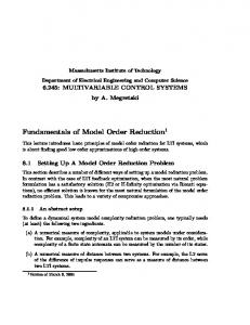
n = 10000, but this time using the inexact version 2-JD. The correction equations (10) are now solved using preconditioned GMRES [13], where a modified incomplete LU factorization of A − θI with drop tolerance 10−3 is used as preconditioner. GMRES is terminated after at most 25 iterations or if the norm of the residual drops below GMRES = 10−3 . If the residual norm in GMRES did not drop below GMRES within 13 iteration steps, the preconditioner is updated. Inexact 2-JD detected 38 dominant eigentriplets within 495 iterations. Most of the detected dominant poles are real and 2-JD had sometimes problems converging to these eigenvalues, hence the relatively high iteration number. One way to improve this behavior could be to use better preconditioners, e.g. using a lower drop tolerance for the incomplete factorizations. However, this will not only increase the computational effort in the algorithm, for general matrix pairs (A, E) it can be difficult to find appropriate incomplete factorizations, especially if E is singular. The Bode plot of exact and reduced order model of order k = 38, as well as the relative error, are given in Figure 2. Again, the exact transfer function is matched very good in the Bode plot, but the relative error is not as small as in the previous example and it becomes worse at higher frequencies.

V. F URTHER GENERALIZATIONS AND ENHANCEMENTS

A. Second order systems The modal truncation approach discussed in Section II can easily be adapted to second order dynamical systems

10−3 −3 10

10−2

10−1

100 Frequency ω

101

102

103

Fig. 2. Bode plot and relative error of exact FDM semi-discretized heat equation model and the k = 38 reduced order model.

of the form  Mx ¨(t) + Dx(t) ˙ + Kx(t) = Bu(t), y(t) = Cx(t),

(11)

with M, D, K ∈ Rn×n . Assuming nonsingular M and K , the transfer function of (11) and its partial fraction expansion is given by [18] 2n X Rj H(s) = C(s M + sD + K)B = , s−λ 2

(12)

j=1

where Rj := (Cxj )(yjH B)λj ∈ Cp×m and (λj , xj , yj ) are eigentriplets of the associated quadratic eigenvalue problems ( Q(λ)x = (λ2 M + λD + K)x = 0, (13) y H Q(λ) = y H (λ2 M + λD + K) = 0. Similar to the first order case, second order dominant poles are now the eigentriplets with a large value of kRj k2 | Re (λj )|. The reduced system is again obtained by projection onto the corresponding right and left dominant eigenspaces: ˜ = Y H M X, D ˜ = Y H DX, K ˜ = Y H KX, M ˜ = Y H B, C˜ = CX. B

(14)

For the intrinsic computation of second order dominant poles one can follow the same principles as in the eigenvalue methods before: projecting the quadratic eigenproblem onto low-dimensional subspaces, solve the resulting small problem with standard methods, and

5

expand the subspaces afterwards via an appropriate correction equation. In a two-sided Jacobi-Davidson style method for (13) the correction equations would read as     pwH pwH Q(θ) I − H f = −Q(λ)v, I− H w p w p (15)     zv H zv H I− H Q(θ)H I − H g = −Q(λ)H w, v z z v where f ⊥ w, g ⊥ v , p := 2θM v + Kv and z := 2θM H w+K H w, see also [6]. The analog to SADPA for second order SISO systems is the Subspace Accelerated Quadratic Dominant Pole Algorithm (SAQDPA) [18] and solves the linear systems Q(θ)f = b, Q(θ)H g = cT instead of (15). A quadratic Rayleigh quotient iteration is also possible, see [18, Alg. 2]. B. Combination with other model reduction techniques In this section we mention a few ways to combine the modal truncation approach of Section II with other modal order reduction approaches in order to get higher accuracies of the reduced order models. Two of the biggest competitors to modal truncation are Krylov subspace interpolation methods and balanced truncation [19]. The dual rational Krylov interpolation via Arnoldi (RKA) [20] is one example for Krylov subspace model order reduction and generates dual rational Krylov subspaces X = Y=

j[ max j=1 j[ max j=1

 Kq (A − σj E)−1 E, (A − σj E)−1 B ,  Kq (A − σj E)−H E T , (A − σj E)−H C T

using multiple interpolation points σ1 , . . . , σjmax ∈ C. Let XRKA , YRKA be matrices containing the right and left basis vectors of such dual rational Krylov subspaces and denote likewise by Xmodal , Ymodal the eigenvector matrices generated by the aforementioned modal truncation approach. One obvious approach to combine them is to use X := [XRKA , Xmodal ] and Y := [YRKA , Ymodal ] as right and, respectively, left projection matrices. Another combination is to use dominant eigenvalues λ1 , . . . , λjmax (or only their real or imaginary parts) as interpolation points for the rational Krylov subspace. Both approaches have already been discussed and tested for first order systems (1) in [14, Ch. 3.8] and for second order system (11) in [18, Ch. 4]. In balanced truncation style model order reduction [19] ones solves the dual Lyapunov equations (assuming E is invertible) AP E T + EP AT = −BB T , T

T

T

A QE + E P A = −C C

(16a) (16b)

and generates projection matrices via −1

−1

XBT := ZP U1 Σ1 2 , YBT := ZQ R1T Σ1 2 , T = Q and Σ , R , U where ZP ZPT = P , ZQ ZQ 1 1 1 are the relevant blocks in the singular value decompoT EZ sition U T ΣR = ZQ P corresponding to the largest T singular values of ZQ EZP . Since the exact solution of (16a),(16b) is not feasible for large-scale systems, one rather computes low-rank-Cholesky factors (LRCFs) T ≈ Q. Z˜P , Z˜C ∈ Rn×k , such that Z˜P Z˜PT ≈ P , Z˜Q Z˜Q This can be achieved with the Generalized Low-RankCholesky-Factor-ADI method (G-LRCF-ADI) [21], [22]. There a LRCF Z˜ is contructed by Z˜ = [Z˜1 , . . . , Z˜imax ], where the block columns Z˜j ∈ Cn×m are generated with the iteration (exemplary for (16a)) p Z˜1 = −2 Re (p1 )(A + p1 E)−1 B, s
Re (pi ) Z˜j = I −(pj +pj−1 )(A+pj E)−1 E Z˜j−1 Re (pi−1 )

for j = 2, . . . , imax . The ADI shift parameters p1 , . . . , pimax ∈ C have significant influence on the convergence speed of this iteration. However, in the context of model order reduction, a fast convergence of G-LRCF-ADI is not the primary goal since it is more important that the generated LRCFs Z˜P , Z˜Q contain enough subspace information in order to approximate the reduced order model accurately enough. This has also been stated in [22, Ch. 4.3.3.], where the author proposed to use dominant poles as shift parameters and the numerical examples [22, Ch. 8.1.4.] confirm this and show interesting results. It is of course also possible to augment the classical, convergence supporting, shifts (for instance the heuristic Penzl shifts [23]) p1 , . . . , pimax by a few dominant poles. VI. C ONCLUDING REMARKS AND FUTURE RESEARCH PERSPECTIVES

The approximation of large-scale linear time invariant systems has become a popular research area in the last decades. We discussed modal approximation as such model order reduction technique, where the reduced order model is obtained by projecting the original system onto the right and left eigenspaces corresponding to the dominant poles of the transfer function. These poles have a significant contribution in the frequency response. Although this idea is relatively simple, it is possible to obtain accurate reduced order models if one has an adequate eigenvalue solver at hand. The two-sided JacobiDavidson method [6] is one promising candidate and its applicability has been investigated. One advantage

6

of this method is its robustness with respect to inexact solves of the involved linear systems. Both the modal approximation approach and the eigenvalue algorithm are easily generalizable to second order systems. There are also various possibilities to combine modal truncation with other reduction methods as is has been discussed for interpolation methods using Krylov subspaces and balanced truncation model order reduction. Both possible combinations encourage further research. R EFERENCES [1] E. J. Davison, “A method for simplifying linear dynamic systems,” vol. AC–11, pp. 93–101, 1966. [2] S. A. Marshall, “An approximate method for reducing the order of a linear system,” Control, vol. 10, pp. 642–643, 1966. [3] N. Martins, L. Lima, and H. Pinto, “Computing dominant poles of power system transfer functions,” IEEE Transactions on Power Systems, vol. 11, no. 1, pp. 162 –170, 1996. [4] J. Rommes and N. Martins, “Efficient computation of transfer function dominant poles using subspace acceleration,” IEEE Transactions on Power Systems, vol. 21, no. 3, pp. 1218 –1226, 2006. [5] A. Stathopoulos, “A case for a biorthogonal Jacobi–Davidson method: Restarting and correction equation,” SIAM Journal on Matrix Analysis and Applications, vol. 24, no. 1, pp. 238–259, 2002. [6] M. E. Hochstenbach and G. L. G. Sleijpen, “Two-sided and alternating Jacobi–Davidson,” Linear Algebra and its Applications, vol. 358(1-3), pp. 145–172, 2003. [7] T. Kailath, Linear Systems, Englewood Cliffs, NJ, 1980. [8] R. Craig and M. Bampton, “Coupling of substructures for dynamic analysis,” AIAA J., vol. 6, pp. 1313–1319, 1968. [9] G. L. G. Sleijpen and H. A. Van der Vorst, “A Jacobi–Davidson iteration method for linear eigenvalue problems,” SIAM Rev., vol. 42, no. 2, pp. 267–293, 2000. [10] A. G. L. Booten, D. R. Fokkema, G. L. G. Sleijpen, and H. A. van der Vorst, “Jacobi–Davidson type methods for generalized eigenproblems and polynomial eigenproblems,” vol. 36, no. 3, 1996. [11] D. R. Fokkema, G. L. G. Sleijpen, and H. A. Van der Vorst, “Jacobi–Davidson style QR and QZ algorithms for the reduction of matrix pencils,” SIAM Journal on Scientific Computing, vol. 20, no. 1, pp. 94–125, 1998. [12] G. H. Golub and C. F. Van Loan, Matrix Computations (3rd ed.). Baltimore, MD, USA: Johns Hopkins University Press, 1996. [13] Y. Saad, Iterative Methods for Sparse Linear Systems. Philadelphia, PA, USA: SIAM, 2003. [14] J. Rommes, “Methods for eigenvalue problems with applications in model order reduction,” Ph.D. dissertation, Universiteit Utrecht, 2007. [15] P. K¨urschner, “Two-sided eigenvalue methods for modal approximation,” Master’s thesis, Chemnitz University of Technology, Department of Mathematics, Germany, 2010. [16] J. Rommes and N. Martins, “Efficient computation of multivariable transfer function dominant poles using subspace acceleration,” IEEE Transactions on Power Systems, vol. 21, no. 4, pp. 1471 –1483, nov. 2006. [17] J. Rommes and G. L. G. Sleijpen, “Convergence of the dominant pole algorithm and Rayleigh quotient iteration,” SIAM Journal on Matrix Analysis and Applications, vol. 30, no. 1, pp. 346–363, 2008.

[18] J. Rommes and N. Martins, “Computing transfer function dominant poles of large-scale second-order dynamical systems,” SIAM Journal on Scientific Computing, vol. 30, no. 4, pp. 2137– 2157, 2008. [19] A. C. Antoulas, Approximation of large–scale dynamical systems. Philadelphia, PA, USA: SIAM, 2005. [20] E. J. Grimme, “Krylov projection methods for model reduction,” Ph.D. dissertation, University of Illinois, 1997. [21] P. Benner, J. R. Li, and T. Penzl, “Numerical solution of large Lyapunov equations, Riccati equations, and linear-quadratic control problems,” Numerical Linear Algebra with Applications, vol. 15, no. 9, pp. 755–777, 2008. [22] J. Saak, “Efficient numerical solution of large scale algebraic matrix equations in PDE control and model order reduction,” Ph.D. dissertation, TU Chemnitz, July 2009. [23] T. Penzl, “A cyclic low rank Smith method for large sparse Lyapunov equations,” vol. 21, no. 4, pp. 1401–1418, 2000.