Model Order Reduction of Parameterized State-Space ...

Model Order Reduction of Parameterized State-Space Systems with Sequential Sampling Elizabeth Rita Samuel, Krishnan Chemmangat, Dirk Deschrijver, Luc Knockaert, Tom Dhaene Department of Information Technology Ghent University - iMinds Gaston Crommenlaan 8 Bus 201 B-9050 Gent Belgium Email: [email protected], [email protected], [email protected], [email protected], [email protected] Abstract—Parameterized reduced order models are important for the design and analysis of microwave structures and systems. Quite often, a large set of models (nodes) with respect to a design parameter variation are uniformly chosen in the parameter design space, which are subjected to model order reduction algorithms and interpolated into a multidimensional model. In order to preserve passivity in the parameterization step, positive interpolation operators are frequently used. This paper demonstrates the importance of sequential sampling for selecting the nodes and building the parameterized models. It is shown that sequential sampling algorithms can significantly reduce the model evaluation cost. The present approach is validated by means of a microstrip example.

I. I NTRODUCTION Sensitivity analysis, design space exploration and optimization of electromagnetic (EM) systems often comes with a significant computational cost (both in terms of CPU time and memory usage). In order to make these tasks feasible, it is worthwhile to build accurate parameterized reduced order models (PROMs) up-front, starting from a large set of system equations. These models are characterized by frequency and several design parameters, such as geometrical or substrate features. Over the past years, a lot of research has been carried out on PROM algorithms [1]–[6]. Well-known techniques like [1], [2] and the two-directional Arnoldi process (PIMTAP) [3] are based on transfer function interpolation. They combine traditional passivity-preserving model order reduction (MOR) methods with interpolation schemes that are based positive interpolation operators [4], [5], [7], [8]. Alternatively, one can resort to state-space matrix interpolation reduced order models (ROMs) [6]. In both cases, it is possible to obtain accurate PROMs that are passive over the complete parameter design space of interest [9]. Most of the PROM techniques are based on the interpolation of univariate nodal macromodels (also called nodes) which are a priori sampled over the parameter design space [10], for example by using rules of thumb that are neither optimal nor automated. One of the main challenges is to find a reduced set of nodes that are well-chosen in the parameter

design space, in order to reduce the model evaluation cost [11]–[14]. In this paper, we show that sequential sampling techniques can facilitate this step and deliver promising results. Sequential sampling techniques can be classified into three main categories, namely input-based methods [15], outputbased methods [13], [16], [17] and model-based methods [11], [12]. In this paper, an algorithm similar to [18] is used for selecting the optimal number of nodes with the aim of generating an accurate PROM. In contrast to the data driven approach presented in [18], additional nodes are selected by comparing the reduced model order of the nodes along the edges of the parameter design space. The advantages of combining a sequential sampling technique [18] along with a PROM technique [9] are numerous: the approach can be applied to multidimensional problems [19], [20], it is portable to parallel computing platforms and it reduces the expensive model evaluation time. The sampling of the parameter design space is fully automated and doesn’t need to be specified a priori, hereby avoiding undersampling/oversampling. Note that undersampling generates poor model quality whereas oversampling often results in waste of computational resources. Finally, it is noted that the local interpolation ensures that the models are stable and passive. The paper is organized as follows. In Section II, the goal statement of parameterized reduced order modeling is discussed briefly. Section III explains the algorithms for model order reduction and state-space interpolation of the nodes. Section IV describes a sequential sampling scheme that demonstrates how the nodes are selected in the parameter design space. A microstrip example is presented in Section V. II. G OAL S TATEMENT Consider a parameterized dynamical system with design parameters ~g = (g (1) , ..., g (N ) ) in descriptor state-space form E(~g )

dx(t, ~g ) = A(~g )x(t, ~g ) + Bu(t) dt y(t, ~g ) = C(~g )x(t, ~g ) + Du(t)

(1)

In the sequel the parameter design space, will be denoted as P(~g ). The goal is to build an interpolated PROM that approximates the large system (1) up to a predefined accuracy level. As a first step, a sequential sampling algorithm is used to identify a set of nodes on a multi-rectangular grid in the parameter design space P(~g ), henceforth called the parameter subspace. These nodes are located at the corner points of each grid cell and correspond to a ROM that characterizes the frequency domain behavior at a fixed point in the parameter design space. Secondly, a parameterization step is introduced to obtain a PROM that can be evaluated at every test point in the parameter design space. This paramaterization is performed by picking the corner points of the corresponding cell and applying local interpolation on the state-space matrices. Regarding the state-space equations of the system under study we assume that a fixed discretization mesh is used which is independent of the specific design parameter values [5]. The size of the system matrices as well as the numbering of the mesh nodes and mesh edges are preserved. The mesh is only locally stretched or shrunk when shape parameters are modified. The matrices B, C are uniquely determined by the circuit topology and therefore remains constant, while the matrices E and A are functions of the design parameters. Starting from a set of models in the design space using common projection matrices, it is straightforward to prove that all the reduced system matrices in the estimation grid are in the same parameter subspace and hence can be interpolated. III. PARAMETERIZED M ODEL O RDER R EDUCTION

UΣV0 = svd(Punion ) A common reduced order r for each node is found by retaining the r most significant singular values as in (2). A common n × r projection matrix Qcomm is obtained as follows: Qcomm = U(:, 1 : r) The congruence transformation using Qcomm , on the original models of the design space then yields the reduced system matrices for all nodes in the specific cell. B. Parameterization by Passive Interpolation In order to obtain a PROM that facilitates the interpolation at an arbitrary position inside the cell, it is possible to apply positive interpolation operators [4] (e.g., multilinear or simplicial methods [21]). Such interpolation schemes have been used extensively in [4], [9] to build stable and passive PROMs. In this paper, multilinear interpolation is applied to the individual state-space matrices (represented by the generic variable J) XK1 XKN J(g (1) , ..., g (N ) ) = ··· J(g(1) ,...,g(N ) ) k1 =1

kN =1

k1

lk1 (g (1) ) · · · lkN (g (N ) )

kN

(4)

Here Ki represents the number of estimation points and lki (g (i) ) are the usual piecewise linear interpolation kernels satisfying 0 ≤ lki (g (i) ) ≤ 1,

A. Model Order Reduction Assuming that a set of M nodes are given, which represent the corner points of a multi-rectangular cell in the parameter design space. In order to interpolate the system response at arbitrary locations inside the cell, a ROM with common model order must be computed for each node. As a first step, a ROM is computed for each node using Krylov-based model order reduction [7], [8] techniques, in our case Laguerre-SVD method [8]. The reduced order of each node qi can be found by computing the ratio of each Hankel singular value σv with respect to the largest singular value σmax and truncating values to zero below a given threshold: σv ≥ thresholdσ , v = 1, 2, ..., q i (2) σmax The choice of the threshold is chosen as a function of the desired accuracy for each ROM. Note that the Hankel singular values quantify the reachability and observability of a system and can be computed by using the command hsvd in Matlab Control System toolbox. After computing the projection matrices for each ROM at the corner points, a common compact projection matrix is found by merging all the columns into a compound matrix [9] : Punion = [P1 , P2 , .....PM ]

SVD is computed for the union of the projection matrices

(3)

The dimension of Punion is n × w where n is the order of the system and w = (q1 + q2 ... + qM ). Next, the economy-size

Ki X

lki (g (i) )

= δki ,i

lki (g (i) )

=1

(5)

k=1

It is important that stability and passivity are guaranteed when a transient analysis is to be performed. It is known that, while a passive system is also stable, the reverse is not necessarily true [22]. Hence the passivity requirement is crucial when the model is to be utilized in a time-domain simulator with drivers and receivers. It is shown in [23] that the passivity of the ROMs is guaranteed if the original models are in the MNA form (1) and if the following conditions are satisfied: E = E0 ≥ 0 A + A0 ≥ 0 B = C0

(6)

For this specific descriptor format, the proposed PROM method guarantees the passivity of the ROMs over the estimation grid using Laguerre-SVD by congruence transformations using the common projection matrix Q :comm Er (~g ) = Qcomm 0 E(~g )Qcomm ≥ 0 Ar (~g ) = Qcomm 0 A(~g )Qcomm ≥ 0 Br (~g ) = Qcomm 0 B(~g ) Cr (~g ) = C(~g )Qcomm

(7)

Fig. 1.

Division of the design space.

Since any nonnegative linear combination of positive semidefinite matrices is positive semidefinite, stability and passivity are preserved over the entire parameter design space. This is the case when positive interpolation operators are used. IV. S EQUENTIAL S AMPLING The division of the parameter design space into multirectangular cells is implemented using a sequential sampling algorithm. Based on differences in the reduced order of each ROM, it is possible to identify the edge of the cell that corresponds to the most dynamic parameter. By selecting additional nodes at the midpoint of that edge, the parameter design space is recursively divided into 2 halves (i.e. 2 smaller subspaces). If the deviation between the original system and the PROM is too large, then the procedure is repeated. Note that this is a key difference with the approach in [18], where the segmentation of the parameter design space is based uniquely on the difference in system responses and the division is performed at the geometric center. As an example, consider a bivariate case with parameter vector ~g = (g (1) , g (2) ) as shown in Fig. 1-a, where the four (1) (2) initial nodes are marked by ~gij = (gi , gj ); i, j = 1, 2. Consider any corner point in the parameter subspace and estimate the reduced order at the corner point and its immediate neighbors in other words, the reduced order has to be estimated for N + 1 points in the parameter subspace, as shown in Fig. 1-b where ~g11 is considered and its immediate neighboring points are [~g12 , ~g21 ]. Next the difference between the reduced orders over each edge is computed, and the PROM is evaluated at the midpoint of the most dynamic edge. At this test node, the difference between the interpolated response of the PROM and the original model is calculated. If the deviation is too large, then the parameter subspace is further divided into two child subspaces along that edge and that procedure is repeated recursively, as shown in Fig. 1-c and Fig.1-d. If the differences across the edges are the same then we can randomly select an edge. Otherwise, if the deviation is sufficiently small and all subspaces are covered, then the algorithm terminates. A flowchart is shown in Fig. 2.

Fig. 2.

Flowchart of sequential sampling algorithm.

Fig. 3.

Layout of five coupled microstrip.

V. E XAMPLE : F IVE C OUPLED M ICROSTRIPS

As an example, five coupled microstrips are considered, where the spacing S between the lines and the length L of the lines are chosen as design parameters in addition to frequency (see Fig. 3). Table I shows the ranges of the parameters and the number of frequency samples Ns is 120. The order of the initial system is 1200. Here, the mean absolute error (MAE) is used as a measure to assess the accuracy of the ROM and −60 dB is used as a target value. If Pin denotes the number of input ports and Pout denotes the number of output ports, then the MAE between the original frequency response Hi,j and the ROM Ri,j is calculated as

TABLE I PARAMETERS OF COUPLED MICROSTRIPS Parameter Frequency (f req) Length (L) Spacing (S)

Min 0 GHz 5 mm 0.04 mm

Max 5 GHz 15 mm 0.1 mm

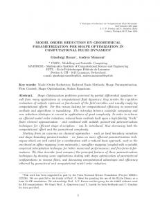
Fig. 5. Fig. 4.

Sequentially sampled design space (validation points marked as ∗)

Hankel singular values of a node.

follows PPin PPout PNs E MAE (~g ) =

i=1

j=1

k=1

|Ri,j (sk , ~g ) − Hi,j (sk , ~g )|

Pin Pout Ns

.

(8) As described in Section III-A, a reduced order of 38 is estimated at the corner point of the parameter design space for L = 5 mm and S = 0.04 mm by truncating the Hankel singular values as shown in Fig. 4. Similarly, the reduced order is estimated for the immediate neighbors of the considered parameter design space and is found to be 44 for L = 5 mm and S = 0.1 mm and 56 for L = 15 mm and S = 0.04. Additional nodes in the design space are selected by the sequential sampling algorithm (see Section IV) and the PROM is generated using multilinear interpolation (see Section III-B). Fig. 5 shows the final result, with as outcome 172 nodes spread in an adaptive non-uniform way. Based on the distribution of the nodes, it can be inferred that S-parameters corresponding to designs with small spacing S and large length L are changing more rapidly. As an illustration, Fig. 6 visualizes the magnitude S18 (L, S) for varying L and S = 0.045 mm. Similarly, in Fig. 7 the magnitude of S16 is shown for varying S with L = 12.8 mm. In both cases, we see that designs with a more resonant-like frequency response are effectively more densely sampled. To validate goodness of fit of the node distribution, the result is compared to a PROM that is build using the same (slightly larger) number of nodes simulated over a classical uniform sampling (e.g., a uniform 14 × 14 grid). The response of the PROMs is evaluated and compared for three validation points, marked by asterisks in Fig. 5. Table II shows a comparison of the MAE over all frequen-

Fig. 6.

Magnitude bivariate PROM S18 (L, S) for S = 0.045 mm.

cies at each validation point. It is clear that the accuracy in the sequential non-uniform case is significantly better than in the uniform case. As a final illustration it can be seen from Fig. 8 that the response of the reduced order model over the sequentially sampled parameter space has a better accuracy than in the uniformly sampled parameter design space case when compared to the original system. VI. C ONCLUSIONS The importance of sequential sampling for building parameterized reduced order models has been demonstrated in this paper. The model is obtained by combining a sequential sampling algorithm that recursively divides the parameter subspace by picking nodes along the most dynamical edge with a local matrix interpolation method. It is shown that an

Fig. 7.

Magnitude bivariate PROM S16 (L, S) for L = 12.8 mm.

Fig. 8. Magnitude of S11 at validation points (uniform and sequential sampling).

TABLE II C OMPARISON OF M EAN A BSOLUTE E RROR L (mm) 8.1 11.7 14.3

S (mm) 0.090 0.070 0.045

Uniform (dB) -66.04 -56.51 -43.91

Sequential (dB) -68.06 -65.12 -62.87

accurate PROM is obtained, while avoiding undersampling or oversampling of the parameter space. The present approach is validated with an example and several numerical results. Due to the curse of dimensionality with the increase in number of parameters, sampling using scattered techniques is being studied. ACKNOWLEDGMENT This work was supported by the Research Foundation Flanders (FWO-Vlaanderen) and by the Interuniversity Attraction Poles Programme BESTCOM initiated by the Belgian Science Policy Office. Dirk Deschrijver is a post-doctoral research fellow of FWO-Vlaanderen. R EFERENCES [1] P. K. Gunupudi, R. Khazaka, M. Nakhla, T. Smy, and D. Celo, “Passive parameterized time-domain macromodels for high-speed transmissionline networks,” IEEE Transactions on Microwave Theory and Techniques, vol. 51, no. 12, pp. 2347 – 2354, Dec. 2003. [2] L. Daniel, O. C. Siong, L. Chay, K. H. Lee, and J. White, “A multiparameter moment-matching model-reduction approach for generating geometrically parameterized interconnect performance models,” IEEE Transactions on Computer-Aided Design of Integrated Circuits and Systems, vol. 23, no. 5, pp. 678 – 693, May 2004. [3] Y.-T. Li, Z. Bai, Y. Su, and X. Zeng, “Model order reduction of parameterized interconnect networks via a two-directional arnoldi process,” IEEE Transactions on Computer-Aided Design of Integrated Circuits and Systems, vol. 27, no. 9, pp. 1571 –1582, Sept. 2008. [4] F. Ferranti, G. Antonini, T. Dhaene, and L. Knockaert, “Guaranteed passive parameterized model order reduction of the partial element equivalent circuit (PEEC) method,” IEEE Transactions on Electromagnetic Compatibility, vol. 52, no. 4, pp. 974–984, Nov. 2010.

[5] F. Ferranti, G. Antonini, T. Dhaene, L. Knockaert, and A. Ruehli, “Physics-based passivity-preserving parameterized model order reduction for PEEC circuit analysis,” IEEE Transactions on Components, Packaging and Manufacturing Technology, vol. 1, no. 3, pp. 399 –409, Mar. 2011. [6] H. Panzer, J. Mohring, R. Eid, and B. Lohmann, “Parametric model order reduction by matrix interpolation,” Automatisierungstechnik, pp. 475–484, Aug. 2010. [7] A. Odabasioglu, M. Celik, and L. Pileggi, “PRIMA: passive reducedorder interconnect macromodeling algorithm,” IEEE Transactions on Computer-Aided Design of Integrated Circuits and Systems, vol. 17, no. 8, pp. 645 –654, Aug. 1998. [8] L. Knockaert and D. De Zutter, “Laguerre-SVD reduced-order modeling,” IEEE Transactions on Microwave Theory and Techniques, vol. 48, no. 9, pp. 1469 –1475, Sept. 2000. [9] E. R. Samuel, F. Ferranti, L. Knockaert, and T. Dhaene, “Parameterized reduced order models with guaranteed passivity using matrix interpolation,” 2012 IEEE 16th Workshop on Signal and Power Integrity,, pp. 65 –68, May 2012. [10] D. Deschrijver and T. Dhaene, “Stability and passivity enforcement of parametric macromodels in time and frequency domain,” IEEE Transactions on Microwave Theory and Techniques,, vol. 56, no. 11, pp. 2435 –2441, Nov. 2008. [11] S. Peik, R. Mansour, and Y. Chow, “Multidimensional Cauchy method and adaptive sampling for an accurate microwave circuit modeling,” IEEE Transactions on Microwave Theory and Techniques,, vol. 46, no. 12, pp. 2364 –2371, Dec. 1998. [12] R. Lehmensiek and P. Meyer, “Creating accurate multivariate rational interpolation models of microwave circuits by using efficient adaptive sampling to minimize the number of computational electromagnetic analyses,” IEEE Transactions on Microwave Theory and Techniques, vol. 49, no. 8, pp. 1419 –1430, Aug. 2001. [13] D. Deschrijver, K. Crombecq, H. Nguyen, and T. Dhaene, “Adaptive sampling algorithm for macromodeling of parameterized S-parameter responses,” IEEE Transactions on Microwave Theory and Techniques, vol. 59, no. 1, pp. 39 –45, Jan. 2011. [14] D. Deschrijver, F. Vanhee, D. Pissoort, and T. Dhaene, “Automated nearfield scanning algorithm for the emc analysis of electronic devices,” IEEE Transactions on Electromagnetic Compatibility,, vol. 54, no. 3, pp. 502 –510, June 2012. [15] K. Crombecq, E. Laermans, and T. Dhaene, “Efficient space-filling and non-collapsing sequential design strategies for simulation-based modeling,” European Journal of Operational Research, vol. 214, no. 3, pp. 683 – 696, Nov. 2011. [16] K. Crombecq, D. Gorissen, D. Deschrijver, and T. Dhaene, “A novel hybrid sequential design strategy for global surrogate modeling of computer experiments,” SIAM Journal on Scientific Computing, vol. 33, no. 4, pp. 1948–1974, Aug. 2011.

[17] S. Aerts, D. Deschrijver, W. Joseph, L. Verloock, F. Goeminne, L. Martens, and T. Dhaene, “Exposure assessment of mobile phone base station radiation in an outdoor environment using sequential surrogate modeling,” Bioelectromagnetics, vol. 34, no. 4, pp. 300–311, 2013. [18] K. Chemmangat, F. Ferranti, T. Dhaene, and L. Knockaert, “Tree-based sequential sampling algorithm for scalable macromodeling of high-speed systems,” 2012 IEEE 16th Workshop on Signal and Power Integrity, pp. 49 –52, May 2012. [19] D. Lewis, “Device model approximation using 2N trees,” IEEE Transactions on Computer-Aided Design of Integrated Circuits and Systems,, vol. 9, no. 1, pp. 30 –38, Jan. 1990. [20] G. P. Fang, D. C. Yeh, D. Zweidinger, L. A. Arledge, and V. Gupta, “Fast, accurate MOS table model for circuit simulation using an unstructured grid and preserving monotonicity,” in Proceedings of the 2005 Asia and South Pacific Design Automation Conference, ser. ASP-DAC ’05. New York, NY, USA: ACM, 2005, pp. 1102–1106. [21] A. Weiser and S. E. Zarantonello, “A note on piecewise linear and multilinear table interpolation in many dimensions,” Mathematics of Computation, vol. 50, no. 181, pp. 189–196, Jan. 1988. [22] R. Rohrer and H. Nosrati, “Passivity considerations in stability studies of numerical integration algorithms,” IEEE Transactions on Circuits and Systems,, vol. 28, no. 9, pp. 857 – 866, Sep. 1981. [23] R. W. Freund, “Krylov-subspace methods for reduced-order modeling in circuit simulation,” J. Comput. Appl. Math., vol. 123, pp. 395–421, Nov. 2000.