Modeling and Control of Nonlinear Networks - Semantic Scholar

Modeling and Control of Nonlinear Networks A Power-Based Perspective

Dimitri Jeltsema

Update: 18th August 2005

Modeling and Control of Nonlinear Networks A Power-Based Perspective

Proefschrift ter verkrijging van de graad van doctor aan de Technische Universiteit Delft, op gezag van de Rector Magnificus Prof.dr.ir. J.T. Fokkema, voorzitter van het College voor Promoties, in het openbaar te verdedigen op 31 mei 2005 om 13:00 uur door Dimitri JELTSEMA elektrotechnisch ingenieur Hogeschool Rotterdam Master of Science in Control Systems Engineering, University of Hertfordshire, United Kingdom geboren te Rotterdam.

Dit proefschrift is goedgekeurd door de promotor: Prof.dr.ir. M. Verhaegen Toegevoegd promotor: Dr.ir. J.M.A. Scherpen Samenstelling promotiecommissie: Rector Magnificus, voorzitter Prof.dr.ir. M. Verhaegen, Technische Universiteit Delft, promotor Dr.ir. J.M.A. Scherpen, Technische Universiteit Delft, toegevoegd promotor Prof.dr. R. Ortega, Sup´elec-LSS Gif-sur-Yvette Prof.dr. A.J. van der Schaft, Universiteit Twente Prof.dr.ir. P.M. Dewilde, Technische Universiteit Delft Prof.dr.techn. A. Kugi, Universit¨at des Saarlandes Dr.ir. J.B. Klaassens, Technische Universiteit Delft Prof.dr. C.W. Scherer, Technische Universiteit Delft (reserve lid)

ISBN 90–8559–048–5 c 2005 by D. Jeltsema Copyright
All rights reserved. No part of the material protected by this copyright notice may be reproduced or utilized in any form or by any means, electronic or mechanical, including photocopying, recording or by any information storage and retrieval system, without written permission from the copyright owner. Cover design by Gemma Plum

Acknowledgments As with playing live music, the support one receives from the audience provides the fuel to perform. The following people have been more than a supporting audience. First of all, it is a great pleasure for me to finally be in the right position to officially thank my supervisor and co-promotor Jacquelien Scherpen, not only for her confidence and the freedom she left me in doing my research, but also for the many valuable hours spend on discussing and structuring my work. Her wise advise and skillful ideas are impressed all over this thesis. I really enjoyed working with her and look forward to many more fruitful discussions in the future. I would like to express my gratitude towards Romeo Ortega who made a very important impact on my thesis. I really appreciate the many illuminating discussions, his valuable ideas, and not to forget the informal time spent together at the Supel´ec barbecue parties. It is simply an honor and a pleasure to work with him. Many thanks to Ben Klaassens. He was one of my first contacts at Delft University of Technology and from the very first day he always enthusiastically supported me and never stopped asking critical and fundamental questions regarding the practical relevance of my work and priorities. I would like to thank Michel Verhaegen for his willingness to be my promotor and for his always adequate response concerning the formalities. Furthermore, I want to thank Arjan van der Schaft. I profited a lot from the useful comments for improvement of this thesis as well as the discussions we had during various phases of my research. I am looking forward to start working together on the Haycon Workpackage 4a project. Many thanks to Carsten Scherer for his many useful and sharp comments. I also like to thank the other members of the promotion committee for their time, comments and interest in my research. I feel truly privileged with my paranimfen and friends for life Gerrit-Frans van Pelt and Marc Scholten. Big up to my brothers in music and beyond: Arjen, Hidde, Sybren, Jeroen, Matthieu and Robby, i.e., the Rotterdam Ska-Jazz Foundation. A v

Acknowledgments loud shout goes out to The Obnoxious R’dam HC Unltd., a state of anarchy formed by Marc, Arie, Aschwin, Leo and myself. Although it has been quite some time ago, I also like to propose a big toast to the members of the Biercommissie and former colleagues at Delft. Hope you are all doing great! Most of all, I want to thank my girl and best friend Gemma to whom this thesis is dedicated. With her infinite love, patience and encouragement she helped me through many difficult moments along the way. Dimitri Jeltsema Rotterdam, April 2005

vi

Contents Acknowledgments

v

Introduction

1

Part I: Nonlinear RLC Networks

9

1

Nonlinear RLC Networks: History, Properties and Preliminaries 1.1 Introduction and Historical Remarks . . . . . . . . . . . . . . 1.2 State Equations and RLC Networks . . . . . . . . . . . . . . . 1.3 Two Common State Formulations . . . . . . . . . . . . . . . . 1.3.1 Current-Voltage Formulation . . . . . . . . . . . . . . 1.3.2 Flux-Charge Formulation . . . . . . . . . . . . . . . . 1.3.3 On the Existence of the State Equations . . . . . . . . 1.3.4 Reciprocity, Passivity and Positivity . . . . . . . . . . 1.4 On the Role of State Functions . . . . . . . . . . . . . . . . . . 1.4.1 Millar’s Content and Co-Content . . . . . . . . . . . . 1.4.2 Cherry’s Energy and Co-Energy . . . . . . . . . . . . . 1.5 The Lagrangian Formulation . . . . . . . . . . . . . . . . . . . 1.5.1 Nonlinear LC Networks . . . . . . . . . . . . . . . . . 1.5.2 Constrained Lagrangian Equations . . . . . . . . . . . 1.5.3 Rayleigh Dissipation . . . . . . . . . . . . . . . . . . . 1.5.4 Stern’s Dissipation Function . . . . . . . . . . . . . . . 1.6 Hamiltonian Formulation . . . . . . . . . . . . . . . . . . . . . 1.6.1 Port-Hamiltonian Systems . . . . . . . . . . . . . . . . 1.6.2 Dissipation . . . . . . . . . . . . . . . . . . . . . . . . 1.7 Retrospection . . . . . . . . . . . . . . . . . . . . . . . . . . . . vii

. . . . . . . . . . . . . . . . . . .

. . . . . . . . . . . . . . . . . . .

. . . . . . . . . . . . . . . . . . .

11 11 14 15 18 18 19 23 25 25 27 29 29 33 34 36 37 38 39 42

Contents 2

3

4

The Brayton-Moser Equations: State-of-the-Art 2.1 Mixed-Potential Modeling . . . . . . . . . . . . . . . . 2.1.1 General Idea . . . . . . . . . . . . . . . . . . . . 2.1.2 Explicit Construction . . . . . . . . . . . . . . 2.2 Stability Theorems . . . . . . . . . . . . . . . . . . . . . 2.2.1 Generation of Lyapunov Function Candidates 2.2.2 The Missing Theorem . . . . . . . . . . . . . . 2.3 From PHD to BM and Back . . . . . . . . . . . . . . . . 2.4 Retrospection . . . . . . . . . . . . . . . . . . . . . . . .

. . . . . . . .

. . . . . . . .

. . . . . . . .

. . . . . . . .

. . . . . . . .

. . . . . . . .

. . . . . . . .

A Novel Passivity Property of RLC Networks: Synthesis and Applications to Stabilization 3.1 Introduction . . . . . . . . . . . . . . . . . . . . . . . . . . . . . . . 3.2 Tellegen’s Theorem and Passivity . . . . . . . . . . . . . . . . . . . . 3.3 A New Passivity Property for RL and RC Networks . . . . . . . . . 3.4 Passivity of Brayton-Moser Networks . . . . . . . . . . . . . . . . . 3.4.1 Framework . . . . . . . . . . . . . . . . . . . . . . . . . . . 3.4.2 Generation of New Storage Function Candidates . . . . . . 3.4.3 Power-Balance Inequality and the New Passivity Property . 3.5 Linear Time-Invariant RLC Networks . . . . . . . . . . . . . . . . . 3.5.1 Preliminaries: Frequency Response Analysis . . . . . . . . 3.5.2 The New Passivity Property and LTI Networks . . . . . . . 3.6 Power-Shaping: A New Paradigm for Stabilization of RLC Networks 3.6.1 Energy-Balancing PBC and Pervasive Dissipation . . . . . 3.6.2 A Motivating Example . . . . . . . . . . . . . . . . . . . . . 3.6.3 Stabilization via Power-Shaping . . . . . . . . . . . . . . . . 3.7 Retrospection . . . . . . . . . . . . . . . . . . . . . . . . . . . . . . .

45 45 46 47 50 52 54 56 60

61 62 63 65 67 67 68 70 73 74 77 82 82 83 84 87

Reactive Hamiltonians: A Paradigm for Reactive Power Compensation 89 4.1 Introduction . . . . . . . . . . . . . . . . . . . . . . . . . . . . . . . 89 4.2 A Reactive Port-Hamiltonian Description . . . . . . . . . . . . . . 90 4.2.1 The New Model . . . . . . . . . . . . . . . . . . . . . . . . . 91 4.2.2 Total Instantaneous Reactive Power . . . . . . . . . . . . . 93 4.3 Towards a Regulation Procedure of Instantaneous Reactive Power . 96 4.4 Input-Output Representation and Passivity . . . . . . . . . . . . . . 99 4.4.1 Input-Output Representation . . . . . . . . . . . . . . . . . 99 4.4.2 Yet Another Passivity Property . . . . . . . . . . . . . . . . 101 4.5 A Different Perspective of PI(D) Control . . . . . . . . . . . . . . . 102 viii

Contents 4.6

Retrospection . . . . . . . . . . . . . . . . . . . . . . . . . . . . . . . 105

Part II: Switched-Mode Power Converters

107

5

. . . . . . . . . . . . . . . . . .

109 109 111 111 113 113 115 116 117 120 121 123 126 127 128 131 134 136 138

. . . . . . . . . . . .

141 141 143 144 147 147 149 151 151 151 153 155 155

6

Power-Based Modeling of Switched-Mode Networks 5.1 Introduction . . . . . . . . . . . . . . . . . . . . . . . 5.2 Ideal Switching Devices . . . . . . . . . . . . . . . . . 5.3 The Switched Brayton-Moser Equations . . . . . . . 5.4 Modeling of DC/DC Converters with Ideal Switches 5.4.1 Boost Converter . . . . . . . . . . . . . . . . 5.4.2 Buck Converter . . . . . . . . . . . . . . . . . 5.5 Networks with Multiple Switches . . . . . . . . . . . . 5.5.1 Phase-to-Phase Description . . . . . . . . . . 5.5.2 Line-to-Line Description . . . . . . . . . . . 5.5.3 Orthogonal Transformations . . . . . . . . . 5.6 Networks with Non-Ideal Switches . . . . . . . . . . . 5.7 Some Issues Regarding Lagrangian Modeling . . . . . 5.7.1 Background . . . . . . . . . . . . . . . . . . . 5.7.2 Problem Formulation . . . . . . . . . . . . . 5.7.3 Equivalent Transfer Impedance . . . . . . . . 5.7.4 Some Other Converter Topologies . . . . . . 5.7.5 Discussion . . . . . . . . . . . . . . . . . . . . 5.8 Retrospection . . . . . . . . . . . . . . . . . . . . . . .

. . . . . . . . . . . . . . . . . .

. . . . . . . . . . . . . . . . . .

Passivity-Based Control in the Brayton-Moser Framework 6.1 Introduction and Motivation . . . . . . . . . . . . . . . . 6.2 Switch Regulation Policy . . . . . . . . . . . . . . . . . . 6.3 EL-Based PBC . . . . . . . . . . . . . . . . . . . . . . . . 6.4 Damping Assignment Revisited: A Motivating Example 6.4.1 Conventional Damping Injection . . . . . . . . . 6.4.2 Parallel Damping Injection . . . . . . . . . . . . 6.5 Power-Based PBC . . . . . . . . . . . . . . . . . . . . . . 6.5.1 Averaged BM Equations . . . . . . . . . . . . . . 6.5.2 Averaged Mixed-Potential Shaping . . . . . . . . 6.5.3 Tuning of the Power-Based PBC . . . . . . . . . 6.5.4 Series/Parallel Damping Injection . . . . . . . . 6.6 Examples of Series Damping Power-Based PBC . . . . . ix

. . . . . . . . . . . . . . . . . .

. . . . . . . . . . . .

. . . . . . . . . . . . . . . . . .

. . . . . . . . . . . .

. . . . . . . . . . . . . . . . . .

. . . . . . . . . . . .

. . . . . . . . . . . . . . . . . .

. . . . . . . . . . . .

. . . . . . . . . . . . . . . . . .

. . . . . . . . . . . .

Contents

6.7

6.8

6.9

6.6.1 The Buck Converter . . . . . . . . . . . . . . . . . 6.6.2 The Boost Converter . . . . . . . . . . . . . . . . . Examples of Parallel Damping Power-Based PBC . . . . . 6.7.1 The Buck Converter . . . . . . . . . . . . . . . . . 6.7.2 The Boost Converter . . . . . . . . . . . . . . . . . 6.7.3 Discussion . . . . . . . . . . . . . . . . . . . . . . . 6.7.4 Numerical Results . . . . . . . . . . . . . . . . . . Power-Based PBC of a Multi-Switch Converter . . . . . . . 6.8.1 Averaged Model . . . . . . . . . . . . . . . . . . . . 6.8.2 Power-Based Control: Parallel Damping Injection 6.8.3 Pre-Compensation Scheme . . . . . . . . . . . . . 6.8.4 Practical Issues . . . . . . . . . . . . . . . . . . . . 6.8.5 Numerical Results . . . . . . . . . . . . . . . . . . Retrospection . . . . . . . . . . . . . . . . . . . . . . . . . .

. . . . . . . . . . . . . .

. . . . . . . . . . . . . .

. . . . . . . . . . . . . .

. . . . . . . . . . . . . .

. . . . . . . . . . . . . .

Part III: Nonlinear Physical Systems 7

8

9

A Novel Power-Based Description of Mechanical Systems 7.1 Introduction and Motivation . . . . . . . . . . . . . . 7.2 Standard Mechanical Systems . . . . . . . . . . . . . . 7.3 Some Examples . . . . . . . . . . . . . . . . . . . . . . 7.3.1 Linear Mass-Spring System . . . . . . . . . . 7.3.2 Spherical Pendulum . . . . . . . . . . . . . . 7.4 On the Role of Dissipation . . . . . . . . . . . . . . . 7.4.1 Mechanical Content and Co-Content . . . . 7.4.2 External Signals . . . . . . . . . . . . . . . . . 7.5 Retrospection . . . . . . . . . . . . . . . . . . . . . . .

156 157 159 159 161 163 164 167 167 168 171 174 175 177

179 . . . . . . . . .

. . . . . . . . .

181 181 186 190 190 192 194 194 197 197

An Energy-Balancing Perspective of IDA-PBC of Nonlinear Systems 8.1 Introduction and Background Material . . . . . . . . . . . . . . . 8.2 A New Passivity Property for a Class of PH Systems . . . . . . . . 8.3 IDA-PBC as an Energy-Balancing Controller . . . . . . . . . . . . 8.4 Some Illustrative Examples . . . . . . . . . . . . . . . . . . . . . . 8.4.1 Connection with Th´evenin-Norton Equivalence . . . . . 8.4.2 Systems Without the Dissipation Obstacle . . . . . . . . . 8.5 Retrospection . . . . . . . . . . . . . . . . . . . . . . . . . . . . . .

. . . . . . .

199 200 204 206 207 207 209 210

Concluding Remarks

. . . . . . . . .

. . . . . . . . .

. . . . . . . . .

. . . . . . . . .

. . . . . . . . .

. . . . . . . . .

213 x

Contents Bibliography

217

Summary

227

Samenvatting

229

Curriculum Vitae

231

xi

Contents

xii

Introduction “The real voyage of discovery consists not in seeking new landscapes but in having new eyes.” Marcel Proust This thesis is focused on the development of new modeling, analysis and control methods for nonlinear electrical networks and physical systems in general.

Motivation A classical, but more actual than ever, problem in modern technology is the optimization, in a suitably defined sense, of the power transfer between the supplier (for example, a generator, accumulator, etc.) and the load (for example, an electronic system). In the area of electrical power conversion, such optimization problems range from simple power management scenarios in mobile phones to complex high-tech devices used in space applications and power plants. In a typical scenario, it is assumed that the supplier consists of a generator with fixed voltage in series with a resistor, and the problem is to design a compensator to minimize the transmission losses. Historically, the loads have been assumed linear, and overwhelmingly inductive. For instance, if the source voltage is purely sinusoidal, it is well-known [26, 15] that the optimal compensator is the one that minimizes the phase shift between the supplied voltage and current waveforms — increasing the so-called power factor. However, we have witnessed in the last two decades an exponential increase in the use of nonlinear electrical apparatus, such as adjustable AC drives and all sort of switching converters, that inject high-frequency harmonics to the power network establishing a non-sinusoidal regime. It is evident that in these circumstances, the power factor compensator design paradigm described above — which is based on sinusoidal steady-state considerations — is not always adequate. In our opinion, a first step towards the construction of a unified frame1

Introduction work for optimization and compensator design that encompasses nonlinear loads, is the development of mathematically tractable and physically sensible methods to analyze and describe the nonlinear phenomena at a level of significant detail. Since virtually all complex physical systems can be viewed as a set of simpler subsystems [105], which exchange power through their mutual interconnections and the environment, it seems natural to take the system’s power as a starting point for the analysis. One of the aims is to construct a unified modeling framework where the total power-flow between the various subsystems is used to play a role similar to well-known energy-based approaches, like the classical Euler-Lagrange and Hamiltonian equations [1, 77, 105]. Once we have obtained such power-based model, it can be used for analysis and then to control the system by modifying the total power to any desired shape as to prescribe a certain desired (dynamical) behavior. If we return to power factor compensator design as briefly described above, this would mean that we start by describing the dynamical behavior of the system in terms of its power-flows. Next, we look what needs to be changed in order to obtain an optimal power transfer, i.e., the desired power-flow. Finally, the power delivered (or extracted) by the controller/compensator is then defined by the difference between the original and the desired power-flow. The key aspect here is that, in contrast to the classical signal-based methods, power does not depend on the form of the signals nor is it restricted to linear elements and systems. This means that the method should be applicable to more general classes of systems, including those from other engineering domains, like mechanical and electro-mechanical (mechatronic) systems. Interestingly, in the early sixties there has already been a relatively small community of researchers which have presented power related ideas in this direction. For example, J.K. Moser [72] was the first who proposed a single power function to model arrays of tunnel diode circuits. Once the model has been obtained, the same function could be used to determine conditions for stability or conditions to maintain stable oscillations. A few years later, a more general theory based on this power function was presented in [10], for which the main result is presently known as the Brayton-Moser equations. From that period on, only a few generalizations where added, and some book writers devoted a chapter on the subject (a detailed list of references can be found in Chapter 2). To our knowledge, none of the authors at that time, nor any of the works from that time on, however, discussed a possible extension of the power-based approach in the direction of control and compensator design. Our objective is to refine and further explore these powerbased concepts to make them suitable for applications and to gain new insights in 2

Introduction modern modeling and control problems. Besides the focus on the power-flows, the key aspect behind our ideas is the notion of passivity.1 Passivity is a fundamental property of dynamical systems that constitutes a cornerstone for many major developments in systems and control theory, including optimal (H 2 and H ∞ ) control, and adaptive control. Passivity has been instrumental to reformulate, in an elegant and unified manner, the central problem of feedback stabilization — either in its form of feedback passivation for general linear and nonlinear systems, or as passivity-based control for systems with physical structures. Passive systems are a class of dynamical systems in which the energy exchanged with the environment plays a central role [77]. In passive systems, the rate at which the energy flows into the system is not less that the increase in storage, i.e., a passive system cannot store more energy than is supplied to it from the outside — with the difference being the dissipated energy. In our approach, passivity will be considered from a fairly different point of view. Instead of a focus on the system’s energy-flows, we focus on the associated power-flow. Our main source of inspiration are the Brayton-Moser equations [10] — including all of its known generalizations — for they constitute a natural dynamical description for a sufficiently large class of nonlinear electrical networks in terms of the systems power-flow.

Contributions and Innovation Several contributions of this thesis can be distinguished. First, a unified powerbased framework for modeling, analysis and control of a large class of nonlinear electrical networks, including switched-mode power converters, is proposed. Second, our research found new power-based passivity properties and lead to the so-called Power-Shaping Stabilization strategy. This new control method forms an alternative to, and is also used to overcome certain obstacles of, the widely appreciated method of Energy-Shaping [80]. Third, we approach the PassivityBased Control (PBC) design methodology for switched-mode power converters, as recently exposed in [77], from a power-based perspective and propose a revised damping injection scenario. This new scenario leads to the notion of parallel damping, which in contrast to series damping results in robust controllers that do not need adaptive extensions to deal with load variations. Additionally, but not less important, effort is made to address the tuning of the controller. Fourth, some 1 Since a list of references concerning passivity can be extended almost indefinitely, the reader is referred to [115, 112, 77, 105] for an excellent expound on the subject and its origins.

3

Introduction preliminary steps are taken to extend the power-based modeling and control ideas to electro-mechanical systems and beyond. Finally, we present some new passivity results for general nonlinear systems which are closely related to the main line of research followed in this thesis. These contributions gave rise to several publications which are explicitly itemized as follows: ✦

In the early sixties Brayton and Moser proved three theorems concerning the stability of nonlinear electrical circuits. The applicability of each theorem depends on three different conditions on the type of admissible nonlinearities in circuit. We provide a natural generalization of Brayton and Moser’s stability theorems that also allows the analysis of a larger class of nonlinear networks. This result has been published in [49].

✦

Our research found new power-based passivity properties and led to the paradigm of Power-Shaping control. This novel control method forms an alternative to, and is also used to overcome certain obstacles of, the widely appreciated method of Energy-Shaping control (presented in e.g. [80]). The new passivity property was presented in [41] and [42]. The extension to stabilization is addressed in the papers [74], [75], and [76].

✦

We have addressed the question when a given RLC network can be rewritten as a port-Hamiltonian (PH) system — with state variables the inductor currents and capacitor voltages instead of the fluxes and charges, respectively. The resulting novel network representation naturally suggests the derivation of a very simple, and physically interpretable, expression for the rate of change of the network’s instantaneous reactive power, and the application to the compensator design paradigm discussed in the previous section. This research is published in [54]. Some related results are published in [13, 39].

✦

The Passivity-Based Control methodology exposed in [77] is rewritten in terms of the Brayton-Moser equations. Based on this framework, practical guidelines for the structure of the injected damping are justified theoretically and the problem of controller commissioning is addressed. The proposed ‘tuning rules’ are shown to be practically relevant in terms of stability, overshoot and non-oscillatory responses. The ideas are exemplified using elementary single-switch and complicated poly-phase power converters. These results were published in [44], [48], and [50]. Some preliminary and related results were published in [51] and [52]. Some results concerning the modeling part were published in [45]. 4

Introduction ✦

Although it is well-known that there is a standard analogy between simple mechanical and electrical systems, like e.g., the mass-inductor or springcapacitor analogy, the existence of a well-defined analogy for more general (electro-)mechanical systems is not straightforward. One of the main reasons for making such analogy difficult is the presence of the so-called coriolis and centrifugal forces in the mechanical domain, which do not appear as such in the electrical domain. Some preliminary findings of extending the power-based modeling and control ideas to electro-mechanical systems and beyond are reported in [46] and [47].

✦

Stabilization of nonlinear feedback passive systems is achieved assigning a storage function with a minimum at the desired equilibrium. For physical systems this has recently led to the so-called Energy-Balancing (EB) control strategy. However, Energy-Balancing stabilization is stymied by the existence of pervasive dissipation, that appears in many engineering applications. The first successful attempt2 to overcome the ‘dissipation obstacle’ is the method of Interconnection and Damping Assignment (IDA), that endows the closed-loop system with a special (port-Hamiltonian) structure. In [40] and [43] we have established a similar equivalence between IDA and EB when the damping is pervasive. Furthermore, we show that the IDA methodology carries on beyond the realm of port-Hamiltonian systems.

Some other contributions which have been inspirational for the developments in present thesis, but are not explicitly included, are the following: ✦

In the context of switched-mode power converter models, we have developed a systematic procedure using the constrained Lagrangian approach. In contrast to earlier methods, our method leads to a set of natural state variables which are directly suitable for application of Passivity-Based Control (PBC). Additionally, we show how to include converter topologies with coupled-magnetics. These contributions are published in [38], [89], and [90].

✦

For complexity reasons, the dynamical behavior of matrix converters are often neglected in controller design. However, increasing demands on reduced harmonic generation and higher bandwidths makes it necessary to study large-signal dynamics. In [53], a unified methodology that considers

2

That is, before the method of Power-Shaping discussed previously.

5

Introduction matrix converters, including input and output filters, as gradient systems is presented. ✦

In [24], we have presented two new choices of regular Lagrangian functions for the dynamical description of LC networks, and prove that the solutions are equivalent one to another and to the results obtained in the literature. The first approach uses the integrated version of Kirchhoff ’s current law (constraints), which is just the condition of charge conservation, to define a regular Lagrangian description by using only the inductances of the system. The second approach is based on the formulation of a Lie algebroid which defines the constraints of the system in a different way. Both approaches are shown to be in a one-to-one relation and they both provide equivalent Hamiltonian formalisms.

Outline of this Thesis This thesis is subdivided into three parts which are structured as follows. Part I contains four chapters which are devoted to general nonlinear RLC networks. The necessary background material is largely contained in Chapter 1 and the first few pages of Chapter 2. It contains a brief historical outline on nonlinear network theory as well as the main concepts and definitions used throughout the thesis. The larger part of Chapter 2 is devoted to Brayton and Moser’s stability theorems and its generalizations. Additionally, some interesting relations between the BraytonMoser equations and port-Hamiltonian systems are established. Chapter 3 is dedicated to the proof that for all RL or RC circuits, and a class of RLC circuits it is possible to ‘add a differentiation’ to one of the port variables (either the voltage or current) preserving passivity, with a storage function that is directly related to the circuit power. The new passivity property naturally suggests the paradigm of Power-Shaping stabilization as an alternative to the well-known method of EnergyShaping. The first part is completed with the development of a port-Hamiltonian description which, in contrast to the standard form, uses an instantaneous reactive power type of Hamiltonian function. This novel network representation naturally suggests the derivation of a very simple, and physically interpretable, expression for the rate of change of the network’s instantaneous reactive power, as well as a procedure for its regulation with external sources. Part II is devoted to the study of switched-mode power converters and contains two chapters. In Chapter 5 the Brayton-Moser equations are accommodated for 6

Introduction the inclusion of (multiple) controllable switches. The approach can be considered as an alternative to the switched Lagrangian and port-Hamiltonian formulation. The theory is exemplified using the elementary single-switch DC/DC Buck and Boost converters, and the more elaborate multi-switch three-phase voltage-source rectifier. Chapter 6 is concerned with the control of switched-mode converters. The chapter starts with an outline of the recently proposed Passivity-Based Control (PBC) methodology. Some new insights regarding the damping assignment philosophy are presented and justified theoretically using the switched versions of Brayton and Moser’s equations. These new insights lead to improvements in the robustness of the closed-loop system against unmodeled load uncertainties. Furthermore, the problem of controller tuning is addressed and extensive simulation studies of the closed-loop behavior are provided. The last part, Part III, is dedicated to the study of more general type of systems in the power-based framework. First, in Chapter 7, the construction of a power-based modeling framework for purely mechanical systems is presented. Finally, in Chapter 8, some equivalence relations between Energy-Balancing (EB) control and Interconnection and Damping Assignment (IDA-PBC) control for general nonlinear systems in which the dissipated power is nonzero at the equilibrium is established.

Notation We denote by ∇x V (·) the partial derivative of a function V : X → R with respect to a n−dimensional column vector x = col(x1 , . . . , xn ) ∈ X, i.e., ∂V (·), ∂x where ∇x V (·) itself represents a column vector. Similarly, the operator ∇x2 denotes the second partial derivative (Hessian) with respect to x, i.e., ∇x V (·) =

∂2 V (·). ∂x2 When clear from the context the subindex will be omitted. ∇x2 V (·) =

Let zˆ : X → Z represent a scalar function mapping x ∈ X unto z ∈ Z. The integral ˆ with respect to x between the endpoints x(1) and x(2) is explicitly written of z = z(x) as

  x(2) V2 x(2) − V1 x(1) = zˆ(x)dx. x(1)

7

Introduction When the lower limit will be taken to be the origin (i.e., x = 0), the latter simplifies to  x V (x) − V (0) = zˆ(x )dx . 0

In many occasions, however, the lower limit of integration need not to be specified until the function is actually evaluated. In such case, we simply write  x V (x) = zˆ(x )dx . The above definitions may be extended to n-dimensional functions provided that the vector field z = zˆ(x) is (locally) symmetric in the sense that ∇zˆ(x) = (∇zˆ(x))T . By an RLC network we refer to an electrical network consisting of arbitrary interconnections of resistors (R), inductors (L), and capacitors (C). The variables related to each of the three elements are labelled by the subindexes r, , and c, respectively. For ease of reference, we often denote the variables related to a currentcontrolled resistor by the subindex r, while for a voltage-controlled resistor we use the subindex g.

8

Part I

Nonlinear RLC Networks

9

Chapter 1

Nonlinear RLC Networks: History, Properties and Preliminaries “Always surpass the one you were yesterday.” Yagyu Sekishusai An entire book could be written on the history of nonlinear network theory starting, roughly speaking, from the early fifties until the present day, with technical explanations, journal and patent references, and interactions with other disciplines. However, its preparation would take more journal and library research than could be justified within the context of the present thesis. In this chapter, we briefly discuss some of the most important developments in nonlinear network theory in relation to our studies in the chapters that follow.

1.1

Introduction and Historical Remarks

Network theory is based on the conceptual modeling of electrical circuits. As in many engineering disciplines, to analyze a complex physical system, we use the description of a system in terms of an ideal model that is an interconnection of idealized elements. The idealized elements are simple models that are used to represent or approximate the properties of separate physical elements or physical phenomena. Although physical elements and physical phenomena may be described in such manner only approximately, idealized elements are by definition characterized precisely. In network theory we study networks made up of idealized elements, and we also study their general properties. Given a physical network, it is possible to obtain a succession of idealized models of this network such that the behavior of the model fits better and better with the physical reality. The ultimate bases 11

Chapter 1. Nonlinear RLC Networks: History, Properties and Preliminaries for the treatment of all electromagnetic phenomena in a physical network are the Maxwell’s equations [66]. However, in a very large number of practical problems, it would mean an unnecessary complication to apply (and moreover, to actually solve) Maxwell’s equations and to describe the behavior of the network under consideration in terms of fields intensities, charge and current densities, etc.. In order to analyze an electrical network it is usually a sufficient approximation to only consider some time-varying quantities satisfying the Maxwell relations, as well as certain incidence and characteristic relations. Going back to Ohm, Kirchhoff, and Maxwell, such approximation has been crucial in the process of understanding the various complex physical phenomena. First, the performance of the individual elements had to be formulated or modeled. The result was Ohm’s law for resistors, Maxwell’s relations for the current and voltage derivatives of the inductors and capacitors, etc.. Secondly, the behavior of interconnected elements had to be formulated. For linear and time-invariant networks, Kirchhoff ’s laws led to linear differential equations expressed in terms of voltages and/or currents, with constant coefficients. Of course, a mathematical theory of such differential equations was well-known at that time, and also its applications to classical mechanics. The popularity and the understanding of the differential equations as they apply to linear networks has led to a wealth of important issues for networks such as steady-state versus transient responses, the superposition theorem, Thevenin’s and Norton’s theorems, and the reciprocity theorem, to mention but a few. All these concepts nowadays belong to the standard outfit of the electrical engineer and can be found in almost any textbook on network theory, design and analysis, e.g., [26]. Until the early 1950s, most researchers only payed attention to the developments of linear network theory. Besides the various fundamental contributions briefly outlined above, there has always been a particular interest in studying the relations between basic equations of mechanics and the basic laws of electrical networks. For generations, many of the results from classical mechanics have been enunciated in terms of the Lagrangian and Hamiltonian formulations of physical systems [1, 2]. A key aspect of these formulations is that they provide a systematic, compact and elegant system description in which physical quantities like energy, interconnection and dissipation play a central role. These results may be translated into network terminology if the networks are properly described. Such translation affords physical insight into the behavior of electrical networks. The use of Lagrange’s equations in the study of electro-magnetic phenomena can be traced back to the era of J.C. Maxwell [66]. However, one of the first researchers that devel12

§1.1. Introduction and Historical Remarks oped a systematic Lagrangian framework for a class of linear networks was Wells [109]. A few years later, Wells also introduced a ‘power function’ — the electrical counterpart of what is known in mechanics as Rayleigh’s dissipation function — in order to account for linear dissipative elements in the network [110]. The field of research took a new turn with the beginning of the era of nonlinear electrical networks, which significantly complicated the analysis. The need for structural nonlinear network analysis was, to our knowledge, first addressed by W. Millar and E.C. Cherry. The main motivation behind the ideas presented in [70], was the search for a generalization of Maxwell’s celebrated minimum heat theorem — one of the first results for linear networks, presented in [66]. Since Maxwell’s minimum heat theorem applies only to linear networks, Millar started to look for some other quantities possessing similar properties in the case of nonlinearities being present in the network. This has led to the notion of resistors content, and its dual, the resistors co-content.1 The second paper [17], accompanying [70], is concerned with the construction of some simple, but fundamental, concepts and theorems related to nonlinear reactance, i.e., nonlinear inductors and capacitors. Cherry introduced the notion of co-energy (the dual of energy) and showed that the equations of motion of a nonlinear network, possessing reactance, may be expressed in Lagrangian form. The inclusion of dissipation and generalized forces (e.g., external voltage and/or current sources) was accomplished using Millar’s content and co-content. The ideas of content and co-content generalized the power function of Wells and enabled the inclusion of nonlinear resistive elements. Since then, many authors contributed to this subject. Besides the structural energy-based methods emphasized here, Brayton and Moser showed that the dynamical equations of a class of nonlinear networks can be expressed in terms of a mixed-potential function, e.g., [10, 11]. The mixed-potential function can be used to prove stability of equilibrium points and reduces to Millar’s content for networks containing no capacitors and to the co-content for networks containing no inductors. The general state-space approach for the time-domain modeling and analysis of nonlinear networks became popular in the late 1950s. For a brief summary on the history of network theory till the early sixties the interested reader is referred to [4]. A selection of papers regarding nonlinear network theory up to 1975 is bundled in [113]. An excellent account of the main results up to 1980 can 1 Millar argued that if there are any nonlinear elements present in a network, the generated heat is in general not stationary at the networks DC operating point. Instead, Millar defined heat related quantities, called content and co-content, which are stationary in the nonlinear case.

13

Chapter 1. Nonlinear RLC Networks: History, Properties and Preliminaries be found in [21]. Another excellent overview up to 1987 is provided in [65]. In the context of the Lagrangian and Hamiltonian formulation some steps of the progress were related to the application of topological methods to justify Cherry’s approach, see e.g., [61] and [99]. Others contributed to the generalization of the Lagrangian and the closely related Hamiltonian descriptions, and to a concept of state variables which came with it. For instance, Chua and McPherson [22] used the classical Lagrangian framework, but their choice of coordinates departed radically from conventional thinking, see also [101]. Almost a decade later, in [58] a generalized Lagrangian (and Hamiltonian) framework is proposed in which some severe limitations of the previous methods are relaxed. In between, Mili´c and Novak [68] introduced the so-called anti-Lagrangian equations and generalized their ideas to nonlinear networks of arbitrary topology in [69]. Some recent contributions on Lagrangian and Hamiltonian formulations of linear and nonlinear networks can be found in e.g., [5, 7, 24, 25, 57, 63, 71], and the references therein.

1.2

State Equations and RLC Networks

The networks considered in our study consist of one-port (or two-terminal) and multi-port (or multi-terminal) resistors, inductors, and capacitors, as well as independent and controlled voltage and current sources. A network, denoted by N , consisting of an arbitrary interconnection of these basic circuit elements is called a dynamic lumped RLC network. For sake of brevity, the time arguments, t ∈ R, of the various dynamic variables are discarded unless stated explicitly otherwise. Basically all developments in this thesis presuppose that the network equations, and physical system equations in general, allow a state equation of the form x˙ = f (x, t),

(1.1)

where x = col(x1 , . . . , xn ) are coordinates, called the state variables of the network, for an n-dimensional state-space manifold Rn , and f : Rn+1 → Rn is a C k vector field for k ≥ 0. Given (1.1), it is well-known that we can in fact define infinitely many equivalent state equations by non-singular coordinate transformations. Of particular interest are the current-voltage formulation, which involve the currents through a set of n inductors, denoted by i , and the voltages across a set of nc capacitors, denoted by uc , respectively, and the flux-charge formulation. The latter formulation involves the flux-linkages p ,  t u (t  )dt  , (1.2) p (t)
p (t0 ) + t0

14

§1.3. Two Common State Formulations with initial conditions p (t0 ), and charges qc , 

t

qc (t)
qc (t0 ) +

ic (t  )dt  ,

(1.3)

t0

with initial conditions qc (t0 ), associated with the inductors and capacitors in the network, respectively. In order to have a clear distinction between the two formulations we denote the state-space of the current-voltage formulation by E∗
I ×Uc , where I represents the space of inductor currents and Uc the space of capacitor voltages, while the state-space of the flux-charge formulation is denoted by E
P × Qc , where P represents the space of inductor flux-linkages and Qc the space of capacitor charges.

1.3

Two Common State Formulations

Any RLC network N containing linear, time-varying and/or nonlinear elements can be represented as shown in Figure 1.1, where all inductors and capacitors are connected externally to a resistive subnetwork M . Since (some of) the inductors (resp. capacitors) may be coupled to each other, multi-port inductors (resp. capacitors) are also included in this representation. Resistors and sources can be regarded as essentially the same kind of elements since they are both specified by static relations in terms of currents and voltages. For example, an independent source may be interpreted as a special case of a one-port resistor, and a controlled source as a special case of a two-port resistor.2 For similar reasons, other oneor multi-port elements, like ideal diodes, switches, transistors (described by the Ebers-Moll equation), gyrators, and transformers, can be considered as resistors, since their constitutive relations are usually also described by algebraic relations involving only currents and voltages and are therefore included in M . To simplify the notation, we assume throughout the thesis that all elements are time-invariant, except possibly the independent sources, and that their constitutive relations can be defined as follows: 2

As argued in [20], there is in fact a sound theoretical reason for this way of classification because it can be proved that any multi-port black box made of arbitrary interconnections of linear resistors, nonlinear resistors, (possibly controlled) voltage- and current sources always gives rise to a multiport resistor. However, there are occasions where it is more convenient to regard these sources as a separate set of elements, especially when we want to specify a particular behavior to them (e.g., if we want to control the circuit or if the network’s passivity properties are considered). We come back to this in later chapters.

15

Chapter 1. Nonlinear RLC Networks: History, Properties and Preliminaries

ia 1 u1

ua1

i1

ub1 ia 2

u2

ic1

ib 1 uc1

ic2

ib 2

Is

ua2

ub2

Es

uc2

i2

ia j uj

ib k

uaj

ick ubk

uck

ij

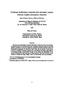
M Fig. 1.1. Any RLC network N can be represented by an algebraic subnetwork M , with port currents iaj , ibk and port voltages uaj , ubk , that is terminated by inductors and capacitors, respectively. The inductors (capacitors) may be coupled to each other.

Definition 1.1 (Resistor) A resistor is an element whose instantaneous current and voltage, denoted by ir ∈ Ir and ur ∈ Ur , respectively, satisfy the relation Γr (ir , ur ) = 0,

(1.4)

called the current-voltage characteristic. A resistor is said to be current-controlled if there exists a function uˆ r : Ir → Ur such that Γr (ir , ur ) = uˆ r (ir ) − ur = 0, or equivalently, ur = uˆ r (ir ). It is voltage-controlled if there exists a function iˆr : Ur → Ir such that ir = iˆr (ur ). A resistor that is both current- and voltage-controlled is a one-toone resistor. For example, a linear resistor is represented by ur = Rir (Ohm’s law), where R is the resistance, or, similarly, ir = Gur , where G (= R−1 ) is the conductance. Hence, a linear resistor is a one-to-one resistor. For ease of presentation, we will often denote a voltage-controlled resistor (a conductor) by the port variables ig and ug , with ig ∈ Ig and ug ∈ Ug , instead of ir and ur , i.e., Γg (ig , ug ) = 0. Definition 1.2 (Inductor) A one-port inductor is an element whose instantaneous 16

§1.3. Two Common State Formulations flux-linkage p ∈ P and current i ∈ I satisfy the relation Γ (p , i ) = 0,

(1.5)

called the flux-current characteristic. An inductor is flux-controlled if there exists a function iˆ : P → I such that Γ (p , i ) = iˆ (p ) − i = 0, or equivalently, i = iˆ (p ). Conversely, it is current-controlled if there exists a function pˆ  : I → P such that p = pˆ  (i ). It is said to be a one-to-one inductor if it is both flux-controlled and current-controlled. Definition 1.3 (Capacitor) A one-port capacitor is an element whose instantaneous charge qc ∈ Qc and voltage uc ∈ Uc satisfy the relation Γc (qc , uc ) = 0,

(1.6)

called the charge-voltage characteristic. A capacitor is charge-controlled if there exists a function uˆ c : Qc → Uc such that Γc (qc , uc ) = uˆ c (qc ) − uc = 0, or equivalently, uc = uˆ c (qc ). Conversely, a capacitor is voltage-controlled if there exists a function qˆc : Uc → Qc such that qc = qˆc (uc ). It is a one-to-one capacitor if it is both chargecontrolled and voltage-controlled. Furthermore, the subnetwork M in Figure 1.1 admits a mixed representation3 of the port voltages ua of the form   hˆ a ia , ub , φs (t) − ua = 0,

(1.7a)

and for the port currents ib   ib − hˆ b ia , ub , φs (t) = 0,

(1.7b)

  where φs (t) = col Es (t), Is (t) represents the possibly time-varying independent voltage and current sources. For autonomous networks, i.e., networks driven by constant (DC) sources, we usually omit the source vector φs . 3

In the work of Chua, e.g., [21], such representations are called hybrid representations, where the word hybrid is used in the sense that the Ohmian relation may be a function of both current and voltage at the same time. We prefer to use the term ‘mixed’ in order to avoid confusion with other closely related fields of research.

17

Chapter 1. Nonlinear RLC Networks: History, Properties and Preliminaries 1.3.1

Current-Voltage Formulation

Let us first consider the current-voltage formulation. Suppose all inductors are current-controlled and the incremental inductance matrix L(i )
∇pˆ  (i )

(1.8)

is non-singular for all i ∈ I . Suppose that all capacitors are voltage-controlled and the incremental capacitance matrix C(uc )
∇qˆc (uc )

(1.9)

is non-singular for all uc ∈ Uc . Substitution of u = −ua into (1.7a) and ic = −ib into (1.7b), yields (see also Figure 1.1)   u = −hˆ a ia , ub , φs (t) ,

  ic = −hˆ b ia , ub , φs (t) .

(1.10)

By Faraday’s law, the inductor voltages equal u = dp /dt = L(i )di /dt, while the capacitor currents equal ic = dqc /dt = C(uc )duc /dt. Furthermore, substitution of i for ia and uc for ub in (1.10) yields    di    = −L−1 (i )hˆ a i , uc , φs (t)     dt (1.11) N :      du c  − 1  = −C (uc )hˆ b i , uc , φs (t) ,  dt which are the state equations on E∗ . Let us define x
col(ia , ub ) = col(i , uc ),      ˆ   ˆh(·)
 ha (·) , and M(·)
 L(·) 0  . (1.12)  ˆ   0 C(·) hb (·) Then, the state equations (1.11) can be represented by the following compact form:   dx = −M −1 (x)hˆ x, φs (t) , dt

(1.13)

ˆ ·) and M(x) are C k -functions, for some k ≥ 0, of x ∈ E∗ . where h( 1.3.2

Flux-Charge Formulation

Let us next derive the flux-charge formulation. For that, the inductors and capacitors need to be flux-controlled and charge-controlled, respectively, so that we may substitute ia = iˆ (p ) and ub = uˆ c (qc ) in (1.7a) and (1.7b), respectively. Hence, by 18

§1.3. Two Common State Formulations noting that dp /dt = −ua and dqc /dt = −ib , we obtain the following state equations on E:  
dp   ˆ a iˆ (p ), uˆ c (qc ), φs (t)  = − h     dt N : (1.14)  
  dq c    = −hˆ b uˆ c (qc ), iˆ (p ), φs (t) . dt Let z
col(p , qc ), then in a similar fashion as before, Eq.’s (1.14) can be represented by the compact form:   dz ˆ = −hˆ x(z), φs (t) , dt

(1.15)

ˆ ·) is a C k -function, for some k ≥ 0, of z ∈ E. where x( 1.3.3

On the Existence of the State Equations

The preceding two state equation formulations are set up deceptively simple beˆ ·) describing the subnetwork M is known a pricause we assumed the function h( ori. For each network, this function must be derived before the state equation can be written, which, in general, is not always possible [21]. Moreover, it is not difficult to give simple examples of pathological networks for which a state equation formulation is even impossible, e.g., a network with a non-invertible currentcontrolled (voltage-controlled) resistor in parallel (series) with a capacitor (inductor). In order to ensure the existence of the solutions for the state equations, either on E∗ or E, we need to confine our study to the class of complete networks expounded below. Definition 1.4 (Completeness) A network N is said to be complete if the state variables x form a complete set of variables. The set of state variables x is complete if its components can be chosen independently without violating Kirchhoff ’s laws4 , and if they determine either the current or the voltage (or both) in every branch of the network. Basically, a network N is complete if the following conditions are satisfied [21, 86]: 4

Kirchhoff ’s current law (KCL) states that for any lumped network, for any of its cutsets, and at any time, the algebraic sum of all the branch currents traversing a branch cut-set is zero. Kirchhoff ’s voltage law (KVL) states that for a lumped network, for any of its loops, and at any time, the algebraic sum of all the branch voltages around a loop is zero.

19

Chapter 1. Nonlinear RLC Networks: History, Properties and Preliminaries C.1 There are no cutsets formed exclusively by inductors and/or independent current sources. There are no loops formed exclusively by capacitors and/or voltage sources. C.2 Each current-controlled (but not voltage-controlled) resistor is in series with an inductor, and each voltage-controlled (but not current-controlled) resistor (i.e., conductor) is in parallel with a capacitor.5 C.3 Each remaining resistor has a bijective characteristic relation. Concerning condition C.1, every inductor-only cutset can usually be eliminated by short-circuiting one of the inductors in the cutset, and by modifying the constitutive relations of the remaining elements in the cutset. Similarly, every capacitoronly loop can be eliminated by open-circuiting any one capacitor in the loop, and by modifying the constitutive relations of the remaining elements in the loop. Most of the fundamental properties of the original elements are inherited by the resulting ‘new’ elements, see e.g., [88]. The same kind of treatment applies to cutsets formed by independent current sources and loops formed by independent voltage sources. Condition C.2 guarantees that the voltage across each current-controlled resistor in series with an inductor is uniquely determined by the inductor current i . Likewise, the current through each voltage-controlled resistor (i.e., conductor) in parallel with a capacitor is uniquely determined by capacitor voltage uc . Condition C.3 guarantees that the resistors not in series or in parallel with an inductor or a capacitor, respectively, are one-to-one which ensures that their constitutive relations can always be expressed in terms of either a current or a voltage. Corollary 1.1 A network N has a global current-voltage formulation (1.13) if it is complete, and the inductors are current-controlled possessing a non-singular incremental inductance matrix of the form (1.8), and the capacitors are voltagecontrolled possessing a non-singular incremental capacitance matrix of the from (1.9). Likewise, the existence of a global flux-charge formulation (1.15) requires the network to be complete with flux-controlled inductors and charge-controlled capacitors. 5 In the multi-port case: Each current-controlled port (or terminal pair) should be in series with an inductor, while each voltage-controlled port (or terminal pair) should be in parallel with a capacitor [21].

20

§1.3. Two Common State Formulations Remark 1.1 Note that in a more general network, where some inductors (capacitors) are current-(voltage-)controlled while others are flux-(charge-)controlled a state formulation is still possible, mutatis-mutandis, by defining a complete set of state variables in an obvious way. Mixed formulations will be used to formulate Lagrange’s equations as treated in Section 1.5. A special subclass of networks that will often be consider in our developments is the class of so-called topologically complete networks.6 Definition 1.5 (Topologically Completeness) A network N is said to be topologically complete if it is complete, and furthermore, if the network N can be decomposed into two subnetworks Na and Nb , where Na contains all inductors and current-controlled resistors, and Nb contains all capacitors and voltage-controlled resistors (i.e., conductors). Basically, a network is topologically complete if all current-controlled resistors are in series with the inductors and all voltage-controlled resistors (conductors) are in parallel with the capacitors. This means that for an autonomous network equations (1.10) take the explicit form  T    u = −Λt uc − Λr uˆ r (Λr i ) −Na − (1.16) N :   ic = ΛT i − ΛT iˆg (Λg uc ) −Nb −. t

g

Observe that ΛTr i = ir and Λg uc = ug , where Λr ∈ Rnr ×n and Λg ∈ Rnc ×ng are constant matrices, express how the currents and voltages in the resistors are related to the independent dynamical variables. The matrix Λt ∈ Rn ×nc can be considered as the ‘turns-ratio’ of a bank of ideal one-to-one transformers connecting the inductive and capacitive elements [99]. Indeed, if we assume for a moment that there are no resistive elements in the network, i.e., Λr = 0 and Λg = 0. Then (1.16) reduces to     u + Λt uc = 0 N : (1.17)   i − ΛT i = 0, c

t 

which clearly constitutes the relationships of an ideal multiple input-output transformer. This agrees with the important fact that the interconnection is lossless and power preserving. We come back to this later on. 6 We have adopted the terminology used in [108]. It should be remarked that the definitions of complete and topologically complete networks are sometimes used in an opposite manner.

21

Chapter 1. Nonlinear RLC Networks: History, Properties and Preliminaries If a network is not topologically complete, we can always try to enlarge the network topology by adding additional dynamic elements — in agreement with the requirements of Definition 1.5 — such that the enlarged network is topologically complete. Let us illustrate this idea using a simple example. uˆ r1 (·) uˆ r2 (·)

uˆ r1 (·) L1

E s1

⇐⇒

uˆ r2 (·) L1

C1 E s1

C1

(a)

(b)

L2 uˆ r2 (·)

M

uˆ r1 (·) L1

E s1

C1 (c)

Fig. 1.2. Network for Example 1.1. (a) A network that is not topologically complete; (b) Subnetwork decomposition (note that M can be considered as a two-port resistor); (c) The addition of an extra inductor renders the network topologically complete.

Example 1.1 Consider the nonlinear RLC network depicted in Figure 1.2(a). Obviously, the network is not topologically complete since the current ir1 cannot be expressed in terms of independent dynamical variables. Suppose that we add an additional inductor, L2 , as shown in Figure 1.2(c). Then, the matrices Λr and Λt are readily found as     −1 0  −1    Λr =   , Λt =   . 1 1 1 Applying Kirchhoff ’s voltage and current law yields the network equations  di    0 = L1 1 − uc1 − ur1    dt  KVL :  (1.18)    di2    0 = L2 − Es1 + uc1 + ur1 + ur2 , dt 22

§1.3. Two Common State Formulations and KCL :

0 = C1

duc1 + i1 − i2 . dt

(1.19)

Since ir1 = i2 − i1 and ir2 = i2 , the enlarged network now is topologically complete. However, in order to find a state formulation for the network of Figure 1.2(a). we need to be able to eliminate the additional current i2 from the above equations. Letting L2 → 0, the second equation in (1.18) reduces to 0 = −Es1 + uc1 + uˆ r1 (i2 − i1 ) + uˆ r2 (i2 )
hˆ a2 (i1 , i2 , uc1 ). The dynamics of the network of Figure 1.2(a) are described implicitly by a set of differential-algebraic equations (DAE’s):   di1  1
   ˆ = + u (i − i ) u c r    1 1 2 1   dt L1        duc1 1
N : (1.20) = i2 − i1    dt C1          0 = hˆ a (i , i , uc ). 2

1

2

1

If hˆ a2 (i1 , i2 , uc1 ) = 0 can be solved7 for i2 such that its solution, i2 = iˆ2 (i1 , uc1 ), is well-defined, then we arrive at an explicit set of ordinary differential equations  di
 1
 1  ˆ (i , uc ) − i  ˆ = + u u i  c r 1 2 1 1 1   L1 1  dt (1.21) N :    duc1 1
ˆ    = i (i , uc ) − i1 .  dt C1 2 1 1 1.3.4

Reciprocity, Passivity and Positivity

Reciprocity A very important network property is the notion of reciprocity. For our purposes, reciprocity is best defined in terms of the symmetry of the incremental parameter matrices. Thus, a multi-port resistor (conductor) described by a C 1 -function is said to be reciprocal iff its associated incremental resistance (conductance) matrix
 R(ir )
∇uˆ r (ir ), G(ug )
∇iˆg (ug ) (1.22) 7 This can be easily checked using the implicit function theorem, which can be found in almost any textbook on advanced calculus or mathematical analysis.

23

Chapter 1. Nonlinear RLC Networks: History, Properties and Preliminaries is symmetric. Reciprocity is defined similarly for inductive and capacitive elements. Of particular interest is the condition for reciprocity of the algebraic subnetwork M of Figure 1.1. Since M consists of one-port or multi-port resistive and/or conductive elements, M itself can be considered as a multi-port resistive and/or conductive element. However, the condition for reciprocity of M is slightly more involved. For ease of notation we assume that M is autonomous. Definition 1.6 The multi-port subnetwork M described by C 1 -functions hˆ a (·) and hˆ b (·) is reciprocal if both the incremental mixed submatrices Haa (·)
∇ia hˆ a (ia , ub ), (1.23)

Hbb (·)
∇ub hˆ b (ia , ub ) are symmetric, and Hab (·)
∇ub hˆ a (ia , ub ),

(1.24)

Hba (·)
∇ia hˆ b (ia , ub ) T (·), for all ia , ub ∈ Rn . are skew-symmetric, i.e., Hab (·) = −Hba

Observe that a one-port element is inherently reciprocal. Thus, the subnetwork M is reciprocal if it contains only one-port resistors and conductors. In case M contains multi-port elements, M is reciprocal iff the elements are reciprocal. However, if M contains a non-reciprocal element, such as a gyrator, M will in general become non-reciprocal. Element Passivity and Positivity A one-port (two-terminal) resistor is passive if its current-voltage characteristic lives in the first and third quadrants, i.e., iTr ur ≥ 0 (see also Figure 1.3), otherwise, it is said to be active. Note that a resistor may possess regions of negative slope and still be passive. A nonlinear resistor is said to be positive if for any two points on the current-voltage characteristic: 

(2) (2) ≥ 0. u(1) i(1) r − ir r − ur It is strictly positive if the latter holds with strict inequality. (Note that the resistor of Figure 1.3 is not positive.) The passivity definition can be extended to multiport resistors. The definition of positivity is extended merely by summing over the terminal pairs [83]. Passivity and positivity is defined similarly for (multi-port) conductive, inductive and capacitive elements. 24

§1.4. On the Role of State Functions

u

I 0

i

III

Fig. 1.3. Characteristic curve of a nonlinear resistor.

1.4

On the Role of State Functions

In the previous section, we have briefly discussed two different sets of state equations describing the dynamical behavior of a large class of (possibly nonlinear) electrical networks. In the chapters that follow we will often make use of special forms describing either one or combinations of the previously defined equations sets (1.13) and/or (1.15). These special forms all make use of certain scalar functions defined on the network’s state-space. The use of state functions in nonlinear network analysis was originated by [17] and [70]. The most familiar examples of such functions are the energies in connection with inductors and capacitors, which will be defined in Subsection 1.4.2. Let us start by introducing the less known concepts of content and co-content.

1.4.1

Millar’s Content and Co-Content

The concepts of content and co-content of a nonlinear resistive type of element was first introduced in [70]. Millar’s original intention seemed to be the search for a generalization of Maxwell’s minimum heat theorem [66] to nonlinear networks. However, the content and co-content functions turned out to be very useful for structural modeling, analysis and control purposes. Definition 1.7 (Content and Co-Content) For any one-port element with charac25

Chapter 1. Nonlinear RLC Networks: History, Properties and Preliminaries

I

u

u

I

G

Is

i

i

(a)

u

(c)

u

Es

G

I G

i

i

(b)

(d)

Fig. 1.4. Content and co-content: (a) The content G and the co-content I are equal to the areas indicated below and above the curve, respectively; (b) Content of a DC voltage source; (c) Cocontent of a DC current source; (d) For a linear element content equals co-content.

ˆ − u = 0, the content G (i) is defined as teristic relation Γ(i, u) = u(i)  G (i)


i

ˆ  )di . u(i

(1.25)

Conversely, for any one-port element that may be characterized explicitly by the ˆ = 0, the co-content I (u) is defined as characteristic relation Γ(i, u) = i − i(u)  u ˆ  )du . I (u)
(1.26) i(u A typical geometrical interpretation of the content and co-content function of various one-port elements is depicted in Figure 1.4. Additionally, we observe that G (i) + I (u) = iu, which shows that the content and co-content are proportional to the power (thus, in case of a resistor, to the generated heat). 26

§1.4. On the Role of State Functions Example 1.2 Consider a linear resistor described by ur = Rir (Ohm’s law). This means that the content is simply half the dissipated power, i.e.,  Gr (ir ) =

ir

1 Rir dir = Ri2r . 2

Similarly, for the co-content, which in case of a linear resistor is defined by Ir (ur ) =




1 2 Gu 2 r

 G = R−1 .

Hence, in the linear case: Gr (ir ) = Ir (ur ) = 12 ir ur (see Figure 1.4 (d)). The above definitions may be extended to multi-port elements, provided that the element is reciprocal, i.e., the gradients of the constitutive relations are symmetric, see Subsection 1.3.4. Reciprocity of the elements is necessary and sufficient to ˆ ˆ and i(u), ensure integrability of u(i) and hence to have G and I , respectively, be state functions. The content and co-content will play a central role in our future developments. Remark 1.2 Millar has generalized the concepts of content and co-content beyond the realm of (reciprocal) elements that allow a functional description in terms of ˆ ˆ or i(u). u(i) From the instantaneous current i(t) and the instantaneous voltage u(t) of an one-port element, the generalized content G (t) is defined as G (t) = G (0) +

 t 0

 di(t  ) u(t )  dt  . dt 

(1.27)

In general, G (t) depends upon the past history of the excitation and so its not a state function — of course, for reciprocal elements it is a state function and is equal to the content defined in (1.25). The co-content can be generalized in a similar way [70]. 1.4.2

Cherry’s Energy and Co-Energy

In the previous subsection we have seen that the dissipated power in any resistive element at any instant can be divided into two parts, the content and the cocontent. In [17] it is shown that similar, yet physically quite distinct, notions arise in connection with inductive and capacitive elements. 27

Chapter 1. Nonlinear RLC Networks: History, Properties and Preliminaries Definition 1.8 (Magnetic Energy and Co-Energy) The magnetic energy, a function of flux-linkage, in a one-port inductive element is  E  (p )


p

iˆ (p )dp ,

(1.28)

and the magnetic co-energy, a function of current, is  E ∗ (i )


i



pˆ  (i )di

 = p i − E  (p ) .

(1.29)

A typical geometrical interpretation of the energy and co-energy function of a oneport inductive element is depicted in Figure 1.5 (a). Γc Γ

E ∗

i

uc

E

E c∗ Ec qc

p (a)

(b)

Fig. 1.5. Energy and co-energy: (a) Inductive element. (b) Capacitive element.

Remark 1.3 Note that the magnetic energy E  (·) may derived from the instantaneous power associated with the inductive element, i.e.,  0

t







i (t )u (t )dt =

 t 0

  p (t) dp (t  )    i (t ) dt = iˆ p (t) dp (t). dt  p (0) 

For the magnetic co-energy E ∗ (·) such power association only holds if the inductor is linear, i.e., when E ∗ (·) = E  (·). Similarly, for a nonlinear capacitive element we have, together with its possible generalizations, the following definition: 28

§1.5. The Lagrangian Formulation Definition 1.9 (Electric Energy and Co-Energy) The electric energy, a function of charge, in an one-port capacitive element is  qc E c (qc )
(1.30) uˆ c (qc )dqc , and the electric co-energy, a function of voltage, is  uc   = qc uc − E c (qc ) . E c∗ (uc )
qˆc (uc )duc

(1.31)

A typical geometrical interpretation of the energy and co-energy function of an one-port capacitive element is depicted in Figure 1.5 (b). The above definitions of energy and co-energy may be extended to multi-port inductive and capacitive elements (with linear or nonlinear mutual coupling), provided that the inductors and capacitors are reciprocal. The (co-)energy functions are found simply by summing over all relevant ports (or terminal pairs) in the definitions. Hence, the total stored (co-)energy of a network is equal to the sum of the (co-)energy stored in each individual inductive and capacitive element.

1.5

The Lagrangian Formulation

The state functions presented in the previous section play an important role in various phases of network theory. The formulation of the network equations in terms of scalar functions provides a compact and elegant description. Equations of this kind are the Lagrangian and Hamiltonian formulations of the network equations, as well as gradient type of descriptions like the Brayton-Moser equations (an extensive list of references is given in the introduction of this chapter). In this section, we briefly discuss some highlights of the Lagrangian modeling approach. We start by considering networks consisting solely of inductors and capacitors, which are characterized by either the energy or co-energy. The inclusion of resistive elements and independent sources is accomplished using the electrical analogue of the Rayleigh dissipation function: the content and co-content. Additionally, it is shown that a peculiar choice of generalized coordinates leads to a special Lagrangian description which coincides with the Brayton-Moser equations. The (port-)Hamiltonian formulation is treated in Section 1.6. 1.5.1

Nonlinear LC Networks

Let N be a network solely composed of n one-port and/or multi-port inductors and nc one-port and/or multi-port capacitors (LC network). Assume that the in29

Chapter 1. Nonlinear RLC Networks: History, Properties and Preliminaries ductors are described by the constitutive relations pˆ j : I → Pj , for j = 1, . . . , n , then the total co-energy stored by the inductors in the network is determined by n  i  j ∗ E  (i ) = pˆ j (. . . , ij , . . .)dij j=1

=

n 

(1.32) ∗

E j (i ).

j=1

Differentiating the latter function with respect to the inductor currents yields ∇E ∗ (i ) = p ⇒ p˙  =

dp d ∗  = ∇E  (i ) = u . dt dt

(1.33)

Furthermore, assume that the capacitors are described by the constitutive relations uˆ ck : Qc → Uck , for k = 1, . . . , nc . The total electric energy stored by the capacitors in the network is determined by nc  qc  k E c (qc ) = uˆ ck (. . . , qck , . . .)dqck k=1

=

nc 

(1.34) E ck (qc ),

k=1

and ∇qc E c (qc ) = uc .

(1.35)

Although there are no resistive and/or conductive elements, the network N can still be represented as shown in Figure 1.1, where the subnetwork M consists solely of a bank of ideal transformers with n × nc ‘turns-ratio’ matrix Λt . For complete networks the topological relationships are explicitly determined by (1.17), which for ease of reference are repeated as: u + Λt uc = 0 (KVL), and ic − ΛTt i = 0 (KCL). Hence, mimicking (KVL) in terms of (1.33) and (1.35) yields d ∗  ∇E  (i ) + Λt ∇E c (qc ) = 0, dt

(1.36)

which is recognized to be closely related to Lagrange’s equation for a conservative mechanical system [1, 2]. Indeed, if we integrate (KCL) with respect to time, we obtain (replacing ic = q˙c and i = q˙ ) by the principle of conservation of charge   t

 t  T    T   q˙c (t ) − Λt q˙ (t ) dt = qc (t ) − Λt q (t )  = 0, 0 0 30

§1.5. The Lagrangian Formulation which, if we assume without loss of generality that the initial conditions are zero, implies that qc = ΛTt q . Hence, if we take the inductor ‘charges’ q as the generalized coordinates, equation (1.36) may be rewritten as  d
∇q˙ L (q , q˙ ) − ∇q L (q , q˙ ) = 0, dt

(1.37)


 where the Lagrangian function is defined as L (q , q˙ )
E ∗ (q˙ ) − E c ΛTt q . Example 1.3 Consider the LC network depicted in Figure 1.6. This example is also used in [5, 63], however, for simplicity we assume that the elements are linear. The matrix Λt is readily found using either one of the Kirchhoff laws (KVL) or (KCL), i.e.,    1 −1 1     0 1 0  (1.38) Λt =  .  0 1 −1    1 0 −1 The Lagrangian for the network is 1 2 1 Lj q˙j − (q + q4 )2 2 j=1 2C1 1 4

L (q , q˙ ) =

−

1 1 (−q1 + q2 + q3 )2 − (−q3 − q4 )2 . 2C2 2C3

Hence, Lagrange’s equations (1.37) read  d2 q1    L  1   dt 2        d2 q2    L  2    dt 2 N :    d2 q3    L 3    dt 2       d2 q     L4 2 4 dt

+

1 1 (q1 + q4 ) − (−q1 + q2 + q3 ) = 0 C1 C2

+

1 (−q1 + q2 + q3 ) = 0 C2

+

1 1 (−q1 + q2 + q3 ) − (−q3 − q4 ) = 0 C2 C3

+

1 1 (q + q4 ) − (−q3 − q4 ) = 0. C1 1 C3

Conversely, if we assume that the capacitors are described by the constitutive relations qˆck : Uc → Qck , for k = 1, . . . , nc , then the total electric co-energy stored 31

Chapter 1. Nonlinear RLC Networks: History, Properties and Preliminaries

L4

C1

L1

L1

L3 C2

C1

⇐⇒

L2

L4

C3

Λt    1 −1 1   0 1 0     0 1 −1    1 0 −1

C2

C3

M

Fig. 1.6. Linear LC network.

by the capacitors in the network is determined by nc  uc  k ∗ E c (uc ) = qˆck (. . . , uck , . . .)duck k=1

=

nc 

(1.39) ∗

E ck (uc ),

k=1

Differentiating the latter function with respect to the voltages yields ∇E c∗ (uc ) = qc ⇒ q˙c =

dqc  d ∗ = ∇E c (uc ) = ic . dt dt

(1.40)

Similarly, if we assume that the inductors are described by the constitutive relations iˆj : P → Ij , for j = 1, . . . , n , then the total energy stored by the inductors in the network is determined by n  p  j E  (p ) = iˆj (. . . , pj , . . .)dpj j=1

=

n 

(1.41) E j (p ).

j=1

Observe that we now have the property ∇E  (p ) = i .

(1.42)

In a similar fashion as before, we try to mimic (KCL) in terms of (1.40) and (1.42), and interpret the integral of (KVL) as some sort of ‘flux-conservation law’, i.e., 32

§1.5. The Lagrangian Formulation p + Λt pc = 0, and consider the variable pc as the ‘capacitor flux’. Indeed, by defining the function L ∗ (pc , p˙ c )
E c∗ (p˙ c ) − E  (−Λt pc ), we obtain  d
∇p˙ c L ∗ (pc , p˙ c ) − ∇pc L ∗ (pc , p˙ c ) = 0. dt

(1.43)

Equations of the form (1.43) are often referred to as co-Lagrangian equations with a Lagrangian co-function L ∗ (pc , p˙ c ). 1.5.2

Constrained Lagrangian Equations

In a mechanical context, EL equations of the form (1.37) represent a generalized force balance. In the electrical domain this means that the equations constitute a voltage balance that corresponds with Kirchhoff voltage law (KVL) — Kirchhoff ’s current law (KCL) is implicitly included in the Lagrangian. The choice of generalized coordinates (inductor ‘charges’), however, seems rather artificial. Similar arguments hold for the co-EL equations (1.43), which constitute a generalized velocity balance. One way to include KCL explicitly in the EL equations (resp., KVL in the co-EL equations) is to consider the constrained EL equations, see e.g., [105], given by  d
˙ − ∇q L (q, q) ˙ = Aλ, ∇q˙ L (q, q) dt

(1.44)

together with the constraint equation8 AT q˙ = 0,

(1.45)

where A is a constant matrix of appropriate dimensions and λ denotes the Lagrange multiplier. The constrained EL equations are accommodated for its application to network modeling by selecting an appropriate set of generalized coordinates. For that, we attach to each energy storage element, i.e., inductor and/or capacitor, two state variables, namely a charge and a current [90]. Physically, it can be viewed as if for the inductor the charge is an intermediate help variable, and for the capacitor the current is. Eliminating the algebraic constraints then finally results in the removal of the intermediate help variables. Indeed, let      q   q˙  q =   , q˙ =   , (1.46) qc q˙c 8 Constraints of this type fall in the class of holonomic constraints, see e.g., [105]. Thus, Kirchhoff ’s current and voltage law can be considered as holonomic constraints. Constraint equations that are not integrable are called non-holonomic.

33

Chapter 1. Nonlinear RLC Networks: History, Properties and Preliminaries then by substitution of A = (Λt | I)T , with I the identity matrix, into (1.44) and solving for λ, yields the network equations (1.17), in the form  dq˙    = −Λt uˆ c (qc ),  L(q˙  )  dt N :     q˙c = ΛTt q˙

L(q˙ ) = ∇2 E ∗ (q˙ ),

(1.47)

For completeness, the constrained version of the co-EL equation can be obtained assigning to each energy storage element both a flux and a voltage coordinate. Hence, equation (1.43) is augmented with  d
˙ − ∇p L ∗ (p, p) ˙ = AT λ∗ , ∇p˙ L ∗ (p, p) dt

(1.48)

and the constraint equation Ap˙ = 0,

(1.49)

or equivalently, replacing pc = uc and solving for λ∗ ,   p˙  = −Λt uc      N :   duc   = ΛTt iˆ (p ), C(uc ) = ∇2 E c∗ (uc ).  C(uc ) dt 1.5.3

(1.50)

Rayleigh Dissipation

Classically, the inclusion of mechanical dissipative elements (e.g., friction) is accomplished using a so-called Rayleigh dissipation function. In the electrical domain, resistive elements are included using a content type of function G : Rn → R such that (1.44) is extended to  d
˙ − ∇q L (q, q) ˙ = Aλ − ∇q˙ G (q), ˙ ∇q˙ L (q, q) dt

(1.51)

while (1.45) remains untouched. Regarding the network representation of Figure 1.1, we directly observe that the subnetwork M should be characterizable solely in ˙ Since the gradient of this function constitutes terms of the content function G (q). a vector of voltages, this means that all elements in M should be strictly currentcontrolled and/or one-to-one. In the linear case this condition is always satisfied. However, more often than not, this will not be the case in nonlinear networks. We come back to such difficulties in Subsection 1.5.4. A similar discussion holds when 34

§1.5. The Lagrangian Formulation we extend (1.48), which involves the inclusion of a co-content type of function I : Rn → R, i.e.,  d
˙ − ∇p L ∗ (p, p) ˙ = AT λ∗ − ∇p˙ I (p). ˙ ∇p˙ L ∗ (p, p) (1.52) dt The subnetwork M should then be characterizable solely in terms of a co-Rayleigh function, i.e., the resistors co-content, requiring that the elements in M are strictly voltage-controlled and/or one-to-one. It should be noted that, in general, the constraints corresponding to KCL (KVL) should be divided between the constraint matrix A and the (co-)content function. In other words, the derivation of the (co)content function may involve the use of KCL (KVL) for determining the current (voltage) associated to a resistive/conductive branch. The remaining constraints thus only involve currents (voltages) associated to the dynamic elements. If there are no such constraints left: set A = 0. Example 1.4 Consider the network depicted in Figure 1.2 (b). The network contains two nonlinear current-controlled resistors characterized by the constitutive relations urj = uˆ rj (irj ), with j = 1, 2, while the remaining elements are linear. We start by assigning to the inductors the (intermediate) variables qj and q˙j , for j = 1, 2, and to the capacitor the variables qc1 and q˙c1 . The Lagrangian for the network is determined by the sum of the co-energy in each inductor minus the energy stored in the capacitor, i.e., L (qc1 , q˙1 , q˙2 ) =

1 2 1 2 1 2 L1 q˙1 + L2 q˙2 − q . 2 2 2C1 c1

(1.53)

The currents through the resistors is completely determined by the inductor currents, hence, the content function is readily found as  q˙ −q˙  q˙ 2 1 2   uˆ r1 (ir2 ) − Es1 dir2 , G (q˙1 , q˙2 ) = (1.54) uˆ r1 (ir1 )dir1 + while the constraint matrix is given by A = (1 −1 | 1)T and λ ∈ R. Substituting the latter into (1.51) yields the following set of implicit differential equations  dq˙    L1 1 = λ + uˆ r1 (q˙2 − q˙1 )    dt        d q˙2    = Es1 − λ − uˆ r1 (q˙2 − q˙1 ) − uˆ r2 (q˙2 )  L2 dt N :     qc1    =λ    C1       0 = q˙1 − q˙2 + q˙ c1 . 35

Chapter 1. Nonlinear RLC Networks: History, Properties and Preliminaries Eliminating the Lagrange multiplier gives  dq˙ qc     L1 1 = 1 + uˆ r1 (q˙2 − q˙1 )    dt C1      dq˙ qc N :  L2 2 = Es1 − 1 − uˆ r1 (q˙2 − q˙1 ) − uˆ r2 (q˙2 )    dt C1       q˙ c1 = q˙2 − q˙1 ,

(1.55)

which coincides with (1.18) and (1.19).

1.5.4

Stern’s Dissipation Function

The above construction has shown that using the Lagrangian formulation, we can concisely summarize the dynamics for a broad class of nonlinear networks in terms of certain scalar state functions. The existence of these functions, and thus of the associated Lagrangian formulation, depend on the type of nonlinearity of the element. The network of Figure 1.2 (b), for example, allowed for a Lagrangian formulation in terms of the inductive co-energy, capacitive energy and a content function playing the role of the Rayleigh function. However, if the resistors are strictly voltage-controlled, or the inductor is strictly flux-controlled such formulation would not be possible. Most of these difficulties associated to the type of nonlinearities of the resistive elements are eliminated if both formulations (1.51) and (1.52) could be somehow combined to one Lagrangian type of equation leading to either state equations of the form (1.11) or (1.14) — depending on the choice of coordinates. Indeed, in [99] it is shown that if we select as generalized velocities the set of independent inductor currents and capacitor voltages (i , uc ) ∈ E∗ (it will turn out that there is no need for the generalized coordinates, i.e., their time-integrals). Assume that the inductors are current-controlled, the capacitors are voltage-controlled, and that the subnetwork M (Figure 1.1) is reciprocal. Let E ∗ (i ) and E c∗ (uc ) denote the total stored inductive and capacitive co-energy, respectively defined in (1.32) and (1.39). Furthermore, assume that there exists a scalar function D : E∗ → R that describes the characteristic of the subnetwork M , i.e.,  D (i , uc ) =

i

 uTa dia −

uc

iTb dub .

(1.56) 36

§1.6. Hamiltonian Formulation Now define the network Lagrangian as the difference between inductive and capacitive co-energy, L (i , uc )
E ∗ (i ) − E c∗ (uc ), and the EL equations become 
 d    ∇i L (i , uc ) = −∇i D (i , uc )     dt N :     d
  ∇uc L (i , uc ) = −∇uc D (i , uc ).  dt

(1.57)

(Compare with (1.11).) Observe that all constraint equations are captured by (1.56), in which the first term is a content type of function and the second term is co-content type of function. In [99], the scalar function (1.56) is referred to as the ‘hybrid dissipation’ function. However, a function of this form was originally introduced in [72] and called ‘mixed-potential’ function. Moreover, Equations (1.57) are a peculiar form of what is known as the Brayton-Moser equations [10, 11]. This formulation will prove itself to be very instrumental for the various developments in the chapters that follow. The explicit construction and philosophy behind the Brayton-Moser equations is discussed in detail in Chapter 2.

1.6

Hamiltonian Formulation

Let N be a network solely composed of n (one-port and/or multi-port) inductors described by the constitutive relations iˆj : P → Ij , for j = 1, . . . , n , and nc (one-port and/or multi-port) capacitors described by the constitutive relations uˆ ck : Q → Uk , for k = 1, . . . , nc . If the network is complete, the state equations in terms of the inductor flux-linkages and capacitor charges, i.e., on the state-space E, can explicitly be written as: dqc = ΛTt iˆ (p ). dt

dp = −Λt uˆ c (qc ), dt

(1.58)

(Compare with (1.17).) Let H : E → R represent the total energy stored in the network, that is H (p , qc ) =

n   j=1

+ =

n  j=1

pj

iˆj (. . . , pj , . . .)dpj

nc   k=1

E j (p ) +

qck

nc 

uˆ ck (. . . , qck , . . .)dqck E ck (qc ),

k=1

37

(1.59)

Chapter 1. Nonlinear RLC Networks: History, Properties and Preliminaries or equivalently, H (z) =

n  

zj

xˆj (. . . , zj , . . .)dzj ,

(1.60)

j=1

where z = col(p , qc ) ∈ E. Then, by noting that ˆ = ∇H (z), x(z)

(1.61)

the network equations (1.58) can compactly be expressed in terms of the energy function as follows: dz = J ∇H (z), dt

(1.62)

where    0 −Λt   .  J
 T Λt 0

(1.63)

In terms of mathematical control theory, the dynamical equations (1.62) with the inductor flux-linkages and capacitor charges as state variables constitute a Hamiltonian system with Hamiltonian function defined as the sum of the inductive and capacitive energy functions of the network, with respect to a Poisson bracket defined on the manifold E by the structure matrix J, see e.g., [63]. For the above equations to be in canonical Hamiltonian form, the number of inductors and the number of capacitors must be equal and Λt must be the identity matrix.9 In such case, the structure matrix J is said to be symplectic [1, 2, 73]. A set of equations of the form (1.62), together with (1.63), is referred to as a generalized Hamiltonian system. An interesting feature of (1.62) is that along the solutions of N dH (z) = 0, dt

(1.64)

which expresses that power is conserved in the network. 1.6.1

Port-Hamiltonian Systems

Recently, the notion of generalized Hamiltonian systems has been extended to the so-called port-Hamiltonian formulation. Port-Hamiltonian systems encompass 9 In [5] a method is proposed to obtain a canonical Hamiltonian formulation using particular state transformations.

38

§1.6. Hamiltonian Formulation a very large variety of physical nonlinear system models [105]. In the context of electrical networks, the philosophy behind the construction of a port-Hamiltonian model is that the elements in the network exchange power (and energy) among each other and the environment through their ports. Indeed, we have already seen in the previous subsection that the inductive and capacitive elements are interconnected through a ‘bank’ of ideal one-to-one transformers. Hence, power between the inductors and capacitors is exchanged through this interconnection and, since the interconnection is lossless, this power is preserved in the network — see (1.64). Suppose now that there are (possibly time-varying) independent sources present in the network, then (1.62) can be extended as dz = J ∇H (z) + Λs φs (·), dt

(1.65)

where the n × ns matrix Λs is called the input matrix. Observe that along the solutions of N we now have that T dH (z)  = ∇H (z) Λs φs (·), dt where the currents and the voltages associated to the independent sources — the so-called ‘natural’ outputs — are determined by    is  dH (z) T = iTs Es (·) + uTs Is (·) = ysT φs (·), (1.66)   = Λs ∇H (z)
ys ⇒ dt us which again expresses power conservation (available network power equals supplied power). Note that the conjugated input-output pair, φs (·) and ys , can be considered as the external ports of the system to which energy can be supplied to or extracted from. A network formulation of the form (1.65), together with outputs ys , i.e.,  dz     = J ∇H (z) + Λs φs (·)  dt (1.67) N :     y = ΛT ∇H (z) s s is called a port-Hamiltonian (PH) system. 1.6.2

Dissipation

Based on the power port concept, additional elements, such as resistors, are easily included terminating (some of) the external ports. Indeed, consider instead of 39

Chapter 1. Nonlinear RLC Networks: History, Properties and Preliminaries Λs φs (·) in (1.67) a term    φs    T  Λs Λr Λg  ur  = Λs φs + Λr ur + ΛTg ig ,   ig and accordingly extend ys to    T  ys   Λs     T   ir  =  Λr  ∇H (z).     ug Λg

(1.68)

(1.69)

Here the pairing ur , ir and ig , ug denote the power variables at the ports which are terminated by (linear) resistive and conductive elements, i.e.,        ur  ˜  ir  ,   = −D (1.70) ig ug ˜ =D ˜ T . Substitution of the latter leads to a portfor some symmetric matrix D Hamiltonian system of the form dz = (J − D)∇H (z) + Λs φs (·), dt

(1.71)

˜ Tr Λg )T is the resistance/conductance matrix. If the resistors where D
(Λr ΛTg )D(Λ and/or conductors are passive, i.e., D = DT ≥ 0, then (1.71) is referred to as a portHamiltonian system with dissipation (PHD) — compare with (1.15) and (1.17). In the previous subsection it was shown that for the case when D = 0, the power-balance dH (z) = ysT φs (·), dt

(1.72)

with ysT φs (·) the power supplied by the indepedent sources. For a network with dissipation (1.71) the power-balance (1.72) extends to T  dH (z) = ysT φs (·) − ∇H (z) D∇H (z), dt

(1.73)

where the second term of the right-hand equation represents the power dissipated by the resistors and conductors. The PHD formulation has the advantage that the network equations are expressed in terms of flux-linkages and charges which directly, and almost always, 40

§1.6. Hamiltonian Formulation lead to a globally defined state equation. On the other hand, it clearly has a disadvantage concerning the admissible class of resistors and conductors. Although, for sake of brevity, we only included linear resistors and/or conductors the largest admissible class is limited to resistors and/or conductors that can be described by a constitutive relation of the form    
  ur  i  T ˜ ˆ T T   = (Λr Λg )D i (p ), uˆ c (qc ) (Λr Λg )    , (1.74) ig 



































































 uc D(z) whereas in general ur and ig are mixed relations: ur = uˆ r (i , uc ) and ig = iˆg (i , uc ). Example 1.5 Consider the topologically complete network of Figure 1.2(c). The Hamiltonian is represented by the total energy stored in the network, i.e., H (p1 , p2 , qc1 ) =

1 2 1 2 1 2 p1 + p2 + q . 2L1 2L2 2C1 c1

Recall that the network contains two nonlinear current-controlled resistors characterized by the constitutive relations urj = uˆ rj (irj ), with j = 1, 2. In order to be able to include these relations they must be such that urj can be decomposed as urj = Rj (. . . , irj , . . .)irj ,

(1.75)

˜ ·) takes the form for some Rj : I → R. In that case, the matrix D(    R1 (ir ) −R1 (ir ) 0   ˜  ) =  −R1 (ir ) R1 (ir ) + R2 (ir ) 0  , D(i   0 0 0 i =ΛT i r

r 

where we subsequently use the fact that i = iˆ (p ) to obtain the dissipation matrix D(p ). Then, the PHD model for the network reads  dp1                0 0 1   dt         dp2       0 0 −1  −    =     dt         −1 1 0   dqc  N :  1     dt            R1 (p ) −R1 (p ) 0   ∇p1 H   0               −R1 (p ) R1 (p ) + R2 (p ) 0   ∇p2 H  +  1 Es1 .             0 0 0 0  ∇qc H  1

41

Chapter 1. Nonlinear RLC Networks: History, Properties and Preliminaries

1.7

Retrospection

In this chapter, we have discussed several fundamental aspects of nonlinear network theory. We have seen that, in general, the study of network theory is based on four fundamental electrical variables, namely, the current, the voltage, the flux, and the the charge. Furthermore, there are three basic network elements defined in terms of the relationship between two of the four fundamental electric variables. The three basic elements are the resistor (defined between current and voltage), the inductor (defined between current and flux), and the capacitor (defined between voltage and charge). A network N made of an arbitrary interconnection of these basic elements is called a dynamic lumped RLC network, or simply an RLC network. Every properly modeled complete RLC network has a well-defined state equation. Depending on the individual element characteristics such state equation is formulated in terms of the inductor currents and capacitor voltages, the inductor flux-linkages and the capacitor charges, or combinations of these variables. A very important concept in network theory is the notion of state functions such as content and co-content, or energy and co-energy. These functions can be used to formulate the dynamic behavior of RLC networks in an elegant, compact and convenient manner. In the last part of this chapter, we have discussed the most well-known examples of state function based modeling concepts: the Lagrangian and (port-)Hamiltonian (PHD) formulations. An overall picture of the connection between the electrical variables, the network elements and the different (state) formulations is shown in Figure 1.7. It is clear that the Lagrangian and co-Lagrangian formulations may be associated to the dashed lines, while the PHD formulation may be associated to the bottom line. The remaining part of the quadrangle (top line) may be associated to the network formulation discussed in Subsection 1.5.4. This particular description is better known as the Brayton-Moser equations, which are discussed in detail in the next chapter. It is of interest to point out that in the nonlinear case the admissible types of dissipation in the PHD framework bear a marked similarity with the definition of the memristor as proposed in [18]. For instance, a one-port charge-controlled memristor is an element characterized by a constitutive relation p = pˆ (q). The corresponding relation between its port voltage and current is given by the Ohmian relation dp/dt = ∇pˆ (q)dq/dt, or u = W(q)i, where W(q)
∇pˆ (q) is called the incremental memristance.10 A memristor as a physical electrical device is, to our 10 A flux-controlled memristor is defined in similar way and is often referred to as a memductance (like a voltage-controlled resistor is often denoted as a conductance).

42

§1.7. Retrospection Brayton-Moser

P

Q

P

Q

I

resistor

U

inductor

U

U

I

U

P

Q

capacitor

I

I

P

?

Q

co-Lagrangian

Lagrangian I

U

P

Q

(port-)Hamiltonian Fig. 1.7. Basic element quadrangle. The ‘?’ could be replaced by memristor type of dissipative elements.

knowledge, still physically undiscovered — apart from realizing its port behavior by operational amplifiers. On the other hand, if one considers mechanical systems, it is easy to see that position dependent friction can be considered as memristor type of phenomena [82]. Memristors can be useful to model various complicated devices. However a detailed discussion is out of place here.

43

Chapter 1. Nonlinear RLC Networks: History, Properties and Preliminaries

44

Chapter 2

The Brayton-Moser Equations: State-of-the-Art “Black fish blue fish old fish new fish.” Dr. Seuss (1960) One particular source of inspiration for the progress of this thesis was the theory expounded in [10] and [11]. For complete reciprocal nonlinear networks, Brayton and Moser proved that it is possible to describe the network as a gradient type of system associated to a single scalar function, called the mixed-potential function. By means of the mixed-potential function, they also constructed several theorems concerning the stability of the network — each with its own particular restriction on the type of admissible nonlinearities. The first part of this chapter reviews the construction of the mixed-potential function up to a level of generality sufficient for the developments in the remaining part of this thesis. In the second part, some generalizations of Brayton and Moser’s stability theorems are provided. This extended family of criteria will appear to be very useful in later chapters. The third and final part of this chapter is devoted to the establishment and study of certain mathematical relations between the Brayton-Moser equations and recent notion of port-Hamiltonian systems, as briefly discussed at the end of the previous chapter.

2.1

Mixed-Potential Modeling

In the early sixties, J.K. Moser [72] developed a mathematical analysis to study the stability of circuits containing tunnel diodes.1 His method was based on the intro1

It should be mentioned that related ideas where already contained in [100].

45

Chapter 2. The Brayton-Moser Equations: State-of-the-Art duction of a certain power-related scalar function, which was four years later generalized and coined mixed-potential by the same author, together with his companion R.K. Brayton in [10] and [11]. For the class of complete networks, Brayton and Moser proved the existence of the mixed-potential function, while for the subclass of topologically complete networks they gave an algorithm for its construction.2 Since then, many generalizations of the mixed-potential are given. For example, in [99] a Lagrangian interpretation of Brayton and Moser’s equations is given, where the mixed-potential is considered as a generalized dissipation function (see also Subsection 1.5.4). In [30], [31] the existence of the mixed-potential for the same classes of networks is proved and an algorithm is given for its construction in terms of a total content and a total co-content function. In [55], [61] the mixed-potential is derived from a variational point a view. The latter observations were proved more rigorously a few years later in [64]. The inclusion of ideal transformers — although this was already discussed years before in [99] — was treated in [36]. For noncomplete networks, Chua [19] explicitly constructed a mixed-potential by using the concept of a pseudo (co-)content and pseudo hybrid content. The problem of finding the largest class of networks for which a mixed-potential can be constructed has been discussed in [62] and [108]. Detailed discussions on the geometrical aspects of the concept of mixed-potential can be found in e.g., [6], [9], [62], [65], and [98]. 2.1.1

General Idea

Basically, the theory of Brayton and Moser is based on the following observation. If the n-port subnetwork M in Figure 1.1 is reciprocal, and each of its branches can (not necessarily uniquely) be determined in terms of its port voltages and currents, then M can be characterized by a single scalar function P : Rn → R. For reciprocal networks this function — the mixed-potential — takes the general form  P (ia , ub ) =

ia

 hˆ Ta (v, w)dv −

ub

hˆ Tb (v, w)dw,

(2.1)

where hˆ a (·) and hˆ b (·) are defined in (1.7a) and (1.7b), respectively (recall that we do not explicitly show the source vector φs (·) in case it is constant). The presence of the minus sign in the right-hand side of the latter equation may seem a little strange at first. Its origin stems from Definition 1.6 and can be explained as follows. Since hˆ a (·) and hˆ b (·) are defined in terms of mixed variables, its associated 2

See Definitions 1.4 and 1.5.

46

§2.1. Mixed-Potential Modeling incremental matrix is not symmetric (see Subsection 1.3.4). Therefore, to define a proper mixed-potential function for M , we need to multiply both sides of (1.7b) ˆ ·) in (1.12) by by minus one and consequently replace h(  ˆ    ˆh∗ (·)
 ha (·)  , ˆ −hb (·) which guarantees that the gradient of hˆ ∗ (·) is symmetric iff M is reciprocal. Thus, for a reciprocal network, hˆ ∗ (·) is integrable for all ia , ub ∈ Rn yielding the mixedpotential function (2.1). Indeed, taking the respective gradients of (2.1), we have by (1.10) that   u = +∇ia P (ia , ub )    a (2.2) M :    i = −∇ P (i , u ). b

2.1.2

ub

a

b

Explicit Construction

In general, the construction of the mixed-potential requires the solution of implicit equations. Simple procedures for its explicit construction, however, can be given for a certain classes of networks. In particular, Brayton and Moser have shown [10] that for topologically complete networks the mixed-potential P : E∗ → R takes the form  i  T   1 Λr uˆ r ΛTr i + Λt uc di P (i , uc ) = 2 (2.3)  uc  T   1 ΛTg iˆg Λg uc − ΛTt i duc , − 2 where we have substituted i = ia and uc = ub (recall that for topologically complete networks, hˆ a and hˆ b are determined by (1.16)). Note that the mixed-potential involves the construction of content and co-content functions. It can be subdivided into a resistive content function Gr : I → R (current potential) associated to the current-controlled resistors in Na ⊆ N , i.e.,  i
 T Gr (i ) = (2.4) Λr uˆ r ΛTr i di and a conductive co-content function Ig : Uc → R (voltage potential) associated to the voltage-controlled resistors in Nb ⊆ N , i.e.,  uc
 T Ig (uc ) = (2.5) ΛTg iˆg Λg uc duc . 47

Chapter 2. The Brayton-Moser Equations: State-of-the-Art The remaining part of the mixed-potential represents the difference between the mixed content and co-content, respectively Gt : E∗ → R and It : E∗ → R, associated to the bank of ideal transformers representing the interconnection between the inductors and capacitors, i.e.,   T 1 i  1 uc
T T  Gt (i , uc ) − It (i , uc ) = −Λt i duc Λt uc di − 2 2 (2.6) T = i Λt uc , where, as before, Λt denotes the ‘turns-ratio’ matrix. This means that (2.3) can be written compactly as P (i , uc ) = Gr (i ) − Ig (uc ) + iT Λt uc ,

(2.7)

while (2.2) in relation to the overall network N takes the form       di         dt   ∇i P (i , uc )      − L(i ) 0       =   N :       .   ) 0 C(u  du c c    ∇ P (i , u )    uc  c  dt

(2.8)

The latter set of equations provide us an elegant way of expressing the dynamical behavior of any network whose resistive portion is reciprocal — and in particular topologically complete. A set of equations of the form (2.8) is referred to as a set of canonical Brayton-Moser (BM) equations. Since L(i ) and C(uc ) are assumed to be non-singular, the state equations can be expressed as  di    = L−1 (i )∇i P (i , uc ) −     dt (2.9) N :    duc  −1  = C (uc )∇uc P (i , uc ).  dt This form simplifies further in three special cases: ✦

(RL networks) If the network does not contain any capacitors, Λt = 0. Furthermore, if all resistors are such that they are contained in the subnetwork Na (i.e., are either current-controlled or one-to-one), then (2.7) reduces to P (i ) = Gr (i ), where the resistive content Gr (i ) is defined in (2.4). Hence, the network equations are −L(i )

di = ∇P (i ). dt

(2.10) 48

§2.1. Mixed-Potential Modeling ✦

(RC networks) Similarly, if the network does not contain any inductors, Λt = 0, and if all resistors are such that they are contained in the subnetwork Nb (i.e., are either voltage-controlled or one-to-one), then (2.7) reduces to P (uc ) = −Ig (uc ), where the conductive co-content Ig (uc ) is defined in (2.5). Thus, the network equations are C(uc )

✦

duc = ∇P (uc ). dt

(2.11)

(LC networks) If the resistors and conductors are absent, we have that Gr = Ig = 0, and thus that P (i , uc ) = Gt (i , uc ) − It (i , uc ) = iT Λt uc . Obviously, the network equations remain of the form (2.8).

Example 2.1 Consider again the topologically complete network of Figure 1.2(c). The network contains two nonlinear current-controlled resistors characterized by the constitutive relations urj = uˆ rj (irj ), with j = 1, 2, while the remaining elements are linear. Hence, the mixed-potential for this network is  P (i1 , i2 , uc1 ) =

i2 −i1

 uˆ r1 (ir1 )dir1 +

i2



 uˆ r2 (ir2 ) − Es1 dir2

+(i1 + i2 )uc1 , (note that Ig = 0) which leads to the following set of differential equations  di    −L1 1 = ∇i1 P = −uc1 − uˆ r1 (i2 − i1 )    dt       di  N : −L2 2 = ∇i2 P = −Es1 + uc1 + uˆ r1 (i2 − i1 ) + uˆ r2 (i2 )   dt        du    C1 c1 = ∇uc1 P = i2 − i1 , dt which coincides with (1.18) and (1.19).

Remark 2.1 Notice that the sum of the mixed content and co-content associated with the bank of ideal transformers representing the interconnection between the inductors and capacitors equals zero, i.e., Gt + It = 0, which expresses the fact that the interconnection is lossless. 49

Chapter 2. The Brayton-Moser Equations: State-of-the-Art Remark 2.2 We can interpret the matrix    −L(i ) 0   
Q(i , uc ) 0 C(uc )

(2.12)

as a pseudo-Riemannian metric on the state-space (i , uc ) ∈ E∗ [104]. Then, the Brayton-Moser equations (2.8) represent a gradient system with respect to this metric and with potential function (2.3). Since the incremental matrices L(i ) > 0 and C(uc ) > 0, the metric is indefinite. If there are no capacitors present (an RL network), or if there are no inductors present (an RC network), then the metric can be taken positive definite.

2.2

Stability Theorems

Apart from being an elegant way of formulating the behavior of a large class of nonlinear networks, the principal use of the concept of the mixed-potential function concerns its use in determining stability criteria for nonlinear networks. Originally, it was Moser’s [72] special interest in finding conditions under which RLC networks containing ‘negative’ resistors such as tunnel diodes do not oscillate, and therefore the trajectories approach the stable equilibria as time increases. For now, let us indicate how the mixed-potential can be advantageously used by considering a network with no capacitors (RL network). In such case, the mixed-potential reduces to P (i ) = Gr (i ), and the Brayton-Moser equations (2.8) reduce to (2.10). Consider then the time-derivative of P (i ) along the trajectories of (2.10):  T T di di di dP
= ∇i P (i ) =− L(i ) . dt dt dt dt

(2.13)

Since L(i ) is positive definite, the network is locally asymptotically stable with Lyapunov function P (i ). If, in addition, the resistors are such that the resistive content has the property Gr (i ) → ∞ as |i | → ∞, then the network is globally asymptotically stable. In general, most RL networks will at least be locally asymptotically stable. Similar conclusions can be drawn for networks with no inductors (RC networks). However, RLC networks will admit self-sustained oscillations and thus marginally stable or even unstable behavior — even in the linear case! One might expect that oscillations can not occur if either the inductors or the capacitors are sufficiently small. Based on the mixed-potential formulation (2.8) Brayton and Moser were 50

§2.2. Stability Theorems able to proof several theorems concerning global asymptotic stability. Two of Brayton and Moser’s stability theorems — Theorem 3 and 4 of [10], respectively (which for ease of reference are stated below as Theorem 2.1 and 2.2, respectively) — give conditions which depend on the interconnection of the circuit as given by the matrix Λt but are independent of the nonlinearities in either the R, L and C elements. Some additional requirements of Theorem 3 and 4 of [10] are that either the Hessian of the current or voltage potentials should be constant and positive definite, i.e., either ∇2 Gr (i ) > 0 and constant or ∇2 Ig (uc ) > 0 and constant. Roughly speaking, this means that either all inductors should have some linear series resistance or all capacitors should have some linear parallel conductance. Theorem 2.1 [10] If R
∇2 Gr (i ) is constant, symmetric and positive definite, Ig (uc ) + |Λt uc | → ∞ as |uc | → ∞, and there exists a δ > 0 such that3 1

1

L 2 (i )R−1 Λt C− 2 (uc ) ≤ 1 − δ,

(2.14)

for all (i , uc ) ∈ E∗ , then all trajectories of (2.8) tend to the set of equilibrium points as t → ∞. Theorem 2.2 [10] If G
∇2 Ig (uc ) is constant, symmetric and positive definite, Gr (i ) + |ΛTt i | → ∞ as |i | → ∞, and there exists a δ > 0 such that 1

1

C 2 (uc )G−1 ΛTt L− 2 (i ) ≤ 1 − δ,

(2.15)

for all (i , uc ) ∈ E∗ , then all trajectories of (2.8) tend to the set of equilibrium points as t → ∞. On the other hand, the third theorem — Theorem 5 of [10] — does not depend on the interconnection matrix Λt but gives conditions which depend on the nonlinearities of the resistors. However, as a dual to the two aforementioned theorems, this theorem requires linearity of both the L and C elements. Let the eigenvalues of a symmetric m × m matrix S(x) be denoted by the set σ(x) = {σ1 (x), . . . , σm (x)}, and let µ(S) represent the infimum of the eigenvalues of S(x) for all x, i.e., " ! µ(S) = inf σj (x) , j = 1, . . . , m. j,x

Theorem 2.3 [10] Under the condition that L and C are constant, symmetric and positive definite, and
1 
1  1 1 µ L− 2 ∇2 Gr (i )L− 2 + µ C− 2 ∇2 Ig (uc )C− 2 ≥ δ, (2.16) 3

The notation · denotes the spectral norm of a matrix.

51

Chapter 2. The Brayton-Moser Equations: State-of-the-Art

Table 2.1. Different assumptions for Brayton and Moser’s stability theorems; linear (LIN) and nonlinear (NL). The column marked with ‘?’ represents the ‘missing’ theorem.

Type

Thm. 3

Thm. 4

Thm. 5

?

R G L/C

LIN NL NL

NL LIN NL

NL NL LIN

NL NL NL

for all δ > 0 and (i , uc ) ∈ E∗ , then all trajectories of (2.8) approach the equilibrium solutions as t → ∞. In summary, Table 2.2 shows the assumptions on the circuit elements regarding the applicability of each of the three theorems above. The column marked with ‘?’ represents the ‘missing’ theorem, i.e., a generalization of the existing three theorems. In the remaining of the section, a new theorem will be proved which omits all possible linearity requirements on the network elements and thus completes Table 2.2. For sake of brevity, Eq’s (2.8) are rewritten in the compact notation Q(x)

dx = ∇P (x), dt

(2.17)

where x ∈ E∗ and Q(x) is defined in (2.12). 2.2.1

Generation of Lyapunov Function Candidates

The underlying idea to proof the stability theorems 2.1, 2.2, and 2.3 (resp., 3, 4, ˜ and P˜ (x), such that (2.17) and 5 of [10]), is the search for an alternative pair, Q(x) can be written as ˜ dx = ∇P˜ (x), Q(x) dt

(2.18)

˜ is negative definite, i.e., and such that the symmetric part of Q(x)  1
˜ + Q˜ T (x) < 0, Q˜ sym (x)
Q(x) 2

(2.19)

for all x. 52

§2.2. Stability Theorems Lemma 2.1 [10] For any arbitrary constant λ and any constant symmetric n × n matrix K, the pair   ˜ = λQ(x) + ∇2 P (x)KQ(x)  Q(x)    (2.20)  T 1     P˜ (x) = λP (x) + ∇P (x) K ∇P (x) 2 is admissible and equivalently characterizes the dynamics (2.17). Proof. Computing the gradient of P˜ (x) gives
 ∇P˜ (x) = λ + ∇2 P (x)K ∇P (x). Since Q(x) is full-rank by assumption, such that −1 ˜ ∇P˜ (x) = Q(x)Q (x)∇P (x),

(2.21)

we conclude that (2.18) is equivalent with (2.17).

Q.E.D.

(More details on the construction of the pairs (2.20) can be found in [10].) The usefulness of Lemma 2.1 is best illustrated as follows. The proof of Theorem 2.1, for example, consists in first selecting λ = −1 and  −1   2R 0   , K =  (2.22) 0 0 and proceeds by verification of (2.14). A simple Schur analysis shows that if (2.14) holds, then negative definiteness of (2.19) is guaranteed. The last step involves the application of LaSalle’s invariance theorem [10]. The proof of the other two theorems follow in a similar way. However, the requirement that K in Lemma 2.1 should be chosen constant is precisely the reason for the several linearity assumptions of the three theorems. Hence, the first step towards a generalization of the theorems is to extend the above procedure to a non-constant K-matrix, i.e., K = K(x). Lemma 2.2 For any arbitrary constant λ and any symmetric n × n matrix K(x), the pair    1
  2 ˜  Q(x) = λQ(x) + ∇ ∇P (x) + ∇ P (x)K(x) Q(x) K(x)    2  (2.23)      1  T   P˜ (x) = λP (x) + ∇P (x) K(x)∇P (x). 2 is admissible and equivalently characterize the dynamics (2.17). 53

Chapter 2. The Brayton-Moser Equations: State-of-the-Art Proof. Like the proof of Lemma 2.1, the extended characterization (2.23) simply follows by noting that    1 1  ∇P˜ (x) = λI + ∇ K(x)∇P (x) + ∇2 P (x)K(x) ∇P (x), 2 2 which, by using (2.21), clearly restores the original description (2.17). Q.E.D. 2.2.2

The Missing Theorem

As discussed before, the original form of Brayton and Moser’s fifth theorem (Theorem 2.3) does not depend on the network interconnection matrix Λt , but it imposes the condition that the inductors and capacitors are linear. Using the theory developed in the previous section, this linearity condition can be omitted as follows. Let  1 1
M1 (x)
∇2 Gr (i ) + ∇i L−1 (i )∇i P L(i ) 2 2 (2.24)  1
−1 1 2 M2 (x)
∇ Ig (uc ) − ∇uc C (uc )∇uc P C(uc ), 2 2 sym

sym

and let M1 (·) and M2 (·) denote their corresponding symmetric parts. Furthermore, let us select a K-matrix and a constant λ in (2.23) as  −1   L (i ) 0  µ − µ1  , λ = 2 , K(x) =  −1 2 0 C (uc ) ˜  ˜  where µ1 = µ M 1 and µ2 = µ M 2 represent the infima of the eigenvalues of the ˜ 1
L−1/2 (i )M sym L−1/2 (i ) and M ˜ 2
C−1/2 (uc )M sym C−1/2 (uc ), respecmatrices M 1 2 tively. Hence, by substituting the latter into (2.23) yields        −M1 (x) −Λt   −L(i ) 0     ˜ =    + λ   Q(x)      ΛTt −M2 (x) 0 C(uc )         T T 1 1    P˜ (x) = λP + ∇i P L−1 (i )∇i P + ∇uc P C−1 (uc )∇uc P , 2 2 which enables us to proof the following theorem. Theorem 2.4 Under the condition that µ1 + µ2 ≥ δ,

δ > 0,

(2.25)

and P˜ (x) → ∞ as |x| → ∞, then all trajectories of (2.17) tend to the set of equilibrium points as t → ∞. 54

§2.2. Stability Theorems Proof. The proof follows along the same lines as the proof of Theorem 5 in [10], and basically consists in evaluating the sign of  T  T dP˜ dx dx ˜ dx ˜ = ∇P (x) = Q(x) dt dt dt dt  T dx ˜ sym dx Q (x) , = dt dt for all x, i.e., we need to show that under condition (2.25) the matrix Q˜ sym (x) is negative definite. Defining I
L1/2 (di )/(dt) and U
C1/2 (duc )/(dt) (for sake of brevity we omit the arguments), one can write 

T   dx ˜ sym dx sym Q (x) = −I T L−1/2 M1 L−1/2 I − dt dt
   sym U T C−1/2 M2 C−1/2 U − λ I T I − U T U
 ˜ 1I − U TM ˜ 2U − λ ITI − U TU = −I T M ≤ −(µ1 + λ)I T I − (µ2 − λ)U T U ≤−

 µ1 + µ2
T I I + U TU 2

< 0, for all I, U
0. This proves the theorem.

Q.E.D.

It is directly noticed that if the inductors and capacitors are linear, the matrices in (2.24) reduce to M1 (i ) = ∇2 Gr (i ) and M2 (uc ) = ∇2 Ig (uc ), respectively. In that case, Theorem 2.4 reduces to Theorem 2.3 (i.e., Theorem 5 in [10]). However, in case of nonlinear inductors and capacitors, the difference between Theorem 2.4 reduces to Theorem 2.3 are the additional terms involving the gradients of L−1 (i ) and C−1 (uc ). We also observe that in contrast to Theorem 2.3, the stability condition of Theorem 2.4 now also depends on the topology of the network since the interconnection matrix Λt now appears in the matrices (2.24), and thus in the stability criterion. Remark 2.3 So far, we have derived a new stability theorem that omits the restrictions imposed by the existing stability theorems originally proposed by Brayton and Moser. The result is mainly based on the generalization of Theorem 2.3. However, the characterization of the pair (2.23) also naturally suggest to generalize Theorem 2.1 and 2.2. This would mean that we have to select the K-matrix in Lemma 55

Chapter 2. The Brayton-Moser Equations: State-of-the-Art 2.2 either as   2    α ∇ Gr (i ) −1 0   , K(·) =   0 0 or

(2.26)

   0  0   K(·) =  −1  ,  2 0 β ∇ Ig (uc )

(2.27)

respectively, where α and β are arbitrary constants. As discussed before, invertibility of ∇2 Gr (i ) (∇2 Ig (uc )) implies that at least every inductor (capacitor) should contain a series (parallel) resistor with a strictly convex constitutive relation. These conditions seem more restrictive than the conditions imposed by Theorem 2.4, but follow along the same lines.

2.3

From PHD to BM and Back

As observed in the previous sections, the mixed-potential function can be built up from contributions of each single one- or multi-port non-energetic element in the subnetwork M (of Figure 1.1), like the energy in the port-Hamiltonian formulation is the sum of the energy associated to each energetic element. It is therefore not so surprising that the Brayton-Moser (BM) equations bear a marked similarity in structure to the port-Hamiltonian (PH, or PHD when dissipation is included) equations discussed in Section 1.6. In view of its practical applications related to controller design, we want to establish a connection between the two formulations and discuss their advantages and disadvantages. The most trivial ‘duality’ is that PH systems requires the inductors and capacitors to be flux- and charge-controlled, while the BM equation impose the restriction that these elements are controlled by the dual variables, namely currents and voltages, respectively. Another duality is that the mixed-potential has the units of power, while the Hamiltonian function has the units of energy. If the formulations are used to design feedback controllers, the controller will consequently rely on some output or state measurements, i.e., measurements of fluxes and charges or currents and voltages. In a practical situation, the off-the-shelf available sensors give as output the measurements in terms of current or voltage quantities only. In the linear case, the relation between flux and current or charge and voltage is an easily obtained bijective relation, but if a system contains nonlinear elements complicated state transformations have to be included or quality degrading approximations have to 56

§2.3. From PHD to BM and Back be made. Since in general the elements may not have bijective relations, it may not even be possible to use one the formulations. One reason to work with PH systems is that the dynamic equations are formulated in physical or ‘natural’ variables [63]. In case of lossless (LC) networks this can be considered a reasonable argument. However, the inclusion of non-energetic elements, like sources and resistors, seems not so natural in the PH framework.4 In principal, the constitutive relations of sources and resistive elements are rather considered in terms of currents or voltages (i.e., in terms of Ohmian relations), instead of fluxes or charges, see e.g., Section 1.3. The inclusion of such elements seems more natural for the BM formalism. Therefore, it is of interest to study if there exists some fundamental relation, in a mathematical sense, between both frameworks. Indeed, as will be shown in the remaining part of this chapter, under some reasonable assumptions such a relation exists. As a consequence, essential and important properties of one framework can be translated to the other. For example, the established relations enable us to translate (already available) controller structures from one framework to the other. Observation 1 Consider a topologically complete linear time-invariant RLC network without any independent sources. The PHD formulation (see Section 1.6) of such network takes the explicit form     dz  0 −Λt   R 0  =  T (2.28)  −   ∇H (z), dt Λt 0 0 G 











































 J −D

where we recall that z ∈ E is a vector containing the inductor fluxes and the capacitor charges, R and G are the resistance and conductance matrices, respectively, and the Hamiltonian H (x) represents the total stored energy, which for linear timeinvariant inductors and capacitors reduces to the quadratic function  −1 1 T  L 0   z. H (z) = z  2 0 C

(2.29)

4

We also remark that, unlike voltage and current whose initial values can be measured at any initial time t0 , Eq.’s (1.2) and (1.3) show that the initial flux p0 initial charge q0 are not measurable quantities and must therefore be prescribed a priori. For that reason, p0 and q0 have no physical significance other than an arbitrary point of reference from which to reckon p and q.

57

Chapter 2. The Brayton-Moser Equations: State-of-the-Art Suppose now that Λt , R, and G are such that J − D is full-rank , then we may rewrite (2.28) as dz (J − D)−1 = ∇H (z). (2.30) dt " ! Furthermore, let Q
J − D. Hence, we actually have two possible pairs, Q , H " ! and (Q )−1 , H , describing the same network dynamics. Inspired by the ideas pre! " sented in Section 2.2.1, the question arises if there exists more pairs, say Q , H  , such that the network dynamics can be written as dz = ∇H  (z). (2.31) dt By Lemma 2.1, such pairs exist under the condition that Q Q ∇H (z) ≡ ∇H  (z) for all z. Now, the key observation is that there is a choice for λ and K in (2.20) such that (2.31) shapes to a set of BM equations. Indeed, if we set λ = 0 and select    R Λt  , K =  T (2.32) Λt −G Q

we observe that (2.31) becomes −1   −L 0  dz   = ∇H  (z), dt 0 C 













(2.33)

Q

where the ‘new’ Hamiltonian H  (z) takes the form 1 1 H  (z) = pT L−1 RL−1 p − qTc C−1 GC−1 qc + pT L−1 Λt C−1 qc . 2 2 



















 





















 























 Gr

(2.34)

Gt −It

Ig

First, we directly notice that Q corresponds to (2.12) in the sense that Q = Q−1 . Second, since L−1 p = i and C−1 qc = uc , we recognize in (2.34) the content and co-content terms (2.4), (2.5), and (2.6). Moreover, the ‘new’ Hamiltonian H  (z) precisely coincides with (2.7) for linear resistors and conductors — with the exception of p and qc . Remark 2.4 Obviously, the above observation also holds for nonlinear networks. In such case, one might need to apply Lemma 2.2, and select a state-dependent Kmatrix, i.e., K = K(z). The main restriction, for both linear or nonlinear networks, is the full rank condition of the J − D matrix. However, if J − D is rank deficient then the network has equilibria at points which are not extrema of the total stored energy. For that reason, the full rank condition seems not restrictive in physical applications. 58

§2.3. From PHD to BM and Back Observation 2 Consider the BM equations (2.17). Since Q(x) is non-singular for all x, we may rewrite (2.17) as dx = Q−1 (x)∇P (x), dt

(2.35)

which directly reveals a marked similarity with the PHD equations (1.71). However, before we may refer to (2.35) as a PHD type of system, we first need to decompose Q−1 (x) into a skew-symmetric and a symmetric matrix which play a role similar to that of the structure matrix J and the dissipation matrix D in the PHD framework. Such decomposition is defined by  1 −1 1    Q (x)
(x) − Q−T (x) J    2 2  Q−1 (x)
J  (x) − D (x) :    1 1    D (x)
− Q−1 (x) − Q−T (x). 2 2

(2.36)

Hence, Eq. (2.35) extends to  dx   = J (x) − D (x) ∇P (x). dt

(2.37)

However, the ‘structure’ matrix J  (x) equals zero since Q−1 (x) is symmetric, while the ‘dissipation’ matrix D (x) is in general indefinite. As we have seen in Section 2.2, we can, using Lemma 2.1, always try to search ! ˜ ˜" for another pair Q, P such that (2.35) can equivalently be described as dx ˜ −1 = Q (x)∇P˜ (x), dt

(2.38)

and such that Q˜ −1 (x) can be decomposed into a (non-zero) skew-symmetric matrix and a (positive semi-definite) symmetric matrix as discussed above. Suppose, for example, that the voltage-controlled resistors (i.e., the conductors) are linear and G is full-rank, and select in Lemma 2.1 λ = 1, and    0 0  K =   , 0 2G−1 then

   −L(i ) 2Λt G−1 C(uc )  ˜   . Q(x) =  −C(uc ) 0

(2.39) 59

Chapter 2. The Brayton-Moser Equations: State-of-the-Art As before, let Q˜ −1 (x)
J˜ (x) − D˜  (x). Hence, the network dynamics can be written in the form  dx
˜ = J (x) − D˜  (x) ∇P˜ (x). dt

(2.40)

Notice that (2.40) is ‘dissipative’ if and only if D˜  (x) ≥ 0, which clearly holds true if the constitutive relations of the network elements are such that Theorem 2.2 is satisfied. In such case, Eq.’s (2.40) constitute a port-Hamiltonian system with dissipation (PHD). Remark 2.5 Since the criteria of Theorem 2.2 determine wether the PHD system (2.40) is ‘dissipative’ or not, we may associate a dissipativity interpretation with the stability condition (2.15). Similar interpretations hold for the conditions of Theorem 2.1 and Theorem 2.3 (as well as Theorem 2.4). See [6], for material closely related with these observations. A dissipativity interpretation of Theorem 2.3 will be of particular interest in Chapter 4.

2.4

Retrospection

In the first part of this chapter, we briefly reviewed the main ideas behind the concept of the mixed-potential function introduced by Brayton and Moser in the early sixties. The second part of this chapter is concerned with the extension of the stability criteria introduced in [10] to a broader class of networks. The key to this result is the generalization of the pair in Lemma 2.1 to the set of pairs in Lemma 2.2. The same lemmata have proven to be useful to establish certain relations, in a mathematical sense, between the Brayton-Moser (BM) equations (‘old fish’) and the port-Hamiltonian (PHD) equations (‘new fish’), as is shown in the third and final part of this chapter. Lemma 2.1 and 2.2 will be of main importance to establish many of our results in the remaining of this thesis. For example, the relationship between the BM and PHD formulations, as outlined for linear time-invariant networks in the previous section, will be particulary useful in Chapter 4 and 7. Furthermore, the idea of writing the PHD equations (2.28) in the non-standard form (2.30) is used in Chapter 7 and 8.

60

Chapter 3

A Novel Passivity Property of RLC Networks: Synthesis and Applications to Stabilization

Arbitrary interconnections of passive (possibly nonlinear) resistors, inductors and capacitors define passive systems, with as power port variables the external sources voltages and currents, and as storage function the total stored energy. In this chapter, we identify a class of nonlinear RLC networks for which it is possible to ‘add a differentiation’ to the port terminals preserving passivity — with a new storage function that is directly related to the network power. For linear networks the new passivity property is characterized in terms of an order relation between the average stored magnetic and electric energy. The results are of interest in networks theory, but also has applications in control as it suggests the paradigm of Power-Shaping stabilization as an alternative to the well-known method of EnergyShaping. Furthermore, in contrast with Energy-Shaping designs, Power-Shaping is not restricted to systems without pervasive dissipation and naturally allows to add ‘derivative’ actions in the control. These important features, that stymie the applicability of Energy-Shaping control, make Power-Shaping very practically appealing. To establish our results we exploit the geometric property that voltages and currents in RLC networks live in orthogonal spaces, i.e., Tellegen’s theorem, and heavily rely on Brayton and Moser’s theorems as presented in the preceding chapter. 61

Chapter 3. A Novel Passivity Property of RLC Networks

3.1

Introduction

Passivity is a fundamental property of dynamical systems that constitutes a cornerstone for many major developments in network and systems theory, see e.g. [33, 105] and the references therein. It is well-known that (possibly nonlinear) RLC networks consisting of arbitrary interconnections of passive resistors, inductors, capacitors and voltage and/or current sources define passive systems with as conjugated port variables the external source voltages and currents, and as storage function the total stored energy [26]. This property was exploited by Youla [115], who proved that terminating the port variables of a passive RLC network with a passive resistor would ensure that ‘finite energy inputs will be mapped into finite energy outputs’, what in modern parlance says that injecting damping to a passive system ensures L2 -stability. Passivity can also be used to stabilize a non-zero equilibrium point, but in this case we must modify the storage function to assign a minimum at this point. If the storage function is the total stored energy this step is referred to as Energy-Shaping, which combined with damping injection constitute the two main stages of Passivity-Based Control (PBC) [79]. As explained in [77, 105], there are several ways to achieve Energy-Shaping, the most physically appealing being the so-called Energy-Balancing PBC (or control by interconnection) method. With this procedure the storage function assigned to the closed-loop passive map is the difference between the total energy of the system and the energy supplied by the controller, hence the name Energy-Balancing. Unfortunately, Energy-Balancing PBC is stymied by the presence of pervasive dissipation, that is, the existence of resistive elements whose power does not vanish at the desired equilibrium point [81]. Another practical drawback of Energy-Balancing control is the limited ability to ‘speed up’ the transient response. Indeed, as tuning in this kind of controllers is essentially restricted to the damping injection gain, the transients may turn out to be somehow sluggish, and the overall performance level below par (see [85] for some representative examples). The main contribution of this chapter is the proof that for all RL or RC networks1 , and a class of RLC networks it is possible to ‘add a differentiation’ to one of the port variables (either voltage or current) preserving passivity, with a storage function that is directly related to the network power. Since the supply rate (the product of the passive conjugated port variables) of the standard passivity property, as defined in e.g. [33, 105], is voltage × current, it is widely known that the 1 It should be mentioned that the result for RL and RC networks was already presented in [78]. This brief note formed the basis for the developments in the present chapter.

62

§3.2. Tellegen’s Theorem and Passivity differential form of the corresponding energy-balance establishes the active powerbalance of the network. Since the new supply rate is voltage × the time-derivative of the current (or current × the time-derivative of the voltage) — quantities which are sometimes adopted as suitable definitions of the supplied reactive power — our result unveils some sort of reactive power-balance. The new passivity property, which is by itself of interest in network theory, has two key features that makes it attractive for control design as well. First, the storage function is not the total energy, but a function directly related with the power in the network. Second, the utilization of power (instead of energy) storage functions immediately suggests the paradigm of Power-Shaping stabilization as an alternative to the method of Energy-Balancing control. It will be shown that, in contrast with Energy-Balancing designs, Power-Shaping is applicable also to systems with pervasive dissipation. The only restriction for stabilization is the degree of (under-)actuation of the network. Further, establishing passivity with respect to ‘differentiated’ port variables allows the direct incorporation of (approximate) derivative actions, whose predictive nature can speed-up the transient response. The chapter is organized as follows. In Section 3.2, we briefly review some fundamental results in networks theory, like the classical definition of passivity and Tellegen’s Theorem. The new passivity property for RL and RC networks is established in Section 3.3. In Section 3.4, this result is extended to the class of RLC networks with convex energy functions and weak electromagnetic coupling using the classical Brayton-Moser equations. In Section 3.5, it will be shown that in case of a linear network the characterization of the new passivity property has a clear interpretation in terms of the phase of the driving point impedance, and an order relationship between the average electric and magnetic energy stored in the network. Finally, in Section 3.6, we present the Power-Shaping stabilization method.

3.2

Tellegen’s Theorem and Passivity

Consider an arbitrary (possibly nonlinear) RLC network which is driven by ns independent (possibly time-varying) voltage and/or current sources. Let us pull out all the independent sources as shown in Figure 3.1 and denote the remaining network by N . In a similar fashion as before, let iγ ∈ Iγ and uγ ∈ Uγ , with ! " γ ∈ r, g, , c , denote the vectors of branch currents and voltages associated to the network elements, respectively. Recall that we may distinguish between two sets of resistors: current-controlled resistors and voltage-controlled resistors, for which the associated currents and voltages are denoted by the subscript ‘r’ and ‘g’, respec63

Chapter 3. A Novel Passivity Property of RLC Networks tively. Linear or one-to-one resistors belong to either one of the two sets. In the this setting, Tellegen’s theorem [83] leads to the observation that  iTs us = iTγ uγ , (3.1) γ

where we have adopted the standard sign convention for the (instantaneous) supplied power iTs us . Thus, at each instant of time the power that enters the network through its ports gets distributed among the elements of the network, so that none is lost [83]. Consequently, equality (3.1) implies that uTs

dis  T diγ = , uγ dt dt γ

us1

(3.2a)

i s1

as well as

N

 duγ = . iTγ is dt dt γ T dus

(3.2b) usk

Another immediate consequence of Tellegen’s theorem is the following, slight variation of the classical result in network theory, see e.g., Section 19.3.3 of [26], whose proof is provided for the sake of completeness.

i sk

Fig. 3.1. Nonlinear RLC network with external power ports.

Proposition 3.1 A network N consisting of arbitrary interconnections of inductors and capacitors with passive resistors verify the energy-balance inequality 









t1

E p (t1 ), qc (t1 ) − E p (t0 ), qc (t0 ) ≤ t0

iTs (t)us (t)dt,

(3.3)

for all t1 ≥ t0 , where E (p , qc ) = E  (p ) + E c (qc ) represents the total stored energy in the network. If, furthermore, the inductors and capacitors are also passive, then N is passive with respect to the supply rate iTs (·)us (·) and storage function the total stored energy. Proof. First, notice that the time-derivative of the total stored energy equals dE (p , qc ) = iT u + iTc uc , dt 64

§3.3. A New Passivity Property for RL and RC Networks where we have used the relations i = ∇E  (p ) and uc = ∇E c (qc ), together with u = dp /dt and ic = dqc /dt. Then, by (3.1), we have that
 dE (p , qc ) = iTs us − iTr ur + iTg ug . dt

(3.4)

Hence, since for passive resistors the dissipated power iTr ur + iTg ug ≥ 0, and integrating (3.4) over the interval [t0 , t1 ], we obtain (3.3). The passivity statement follows from non-negativity of the total stored energy E (p , qc ) for passive inductors and capacitors. Q.E.D. In other words, for passive networks the total stored energy is just a non-negative2 function which increases along the trajectories more slowly than the rate at which energy is supplied through the external ports (or decreases more rapidly than the rate at which energy is extracted from the ports).

3.3

A New Passivity Property for RL and RC Networks

In the remaining of this chapter, our aim is to consider passivity from a different perspective using the networks power flow instead of the total stored energy. To illustrate the basic idea of the new passivity properties, we first consider networks consisting solely of inductors, resistors and independent sources, i.e., RL networks N(C=) , and networks consisting solely of capacitors, resistors and independent sources, i.e., RC networks N(L=) . The results will be generalized to a class of RLC networks in the following sections. For ease of reference, let us recall some additional definitions and concepts which will be instrumental to formulate our results. Recall from Chapter 1, Definition 1.7, that to a set of reciprocal (one- or multi-port) nonlinear current-controlled resistors (this includes linear or one-toone resistors as special cases) we may associate a scalar function Gr : Ir → R, called the resistor’s content. Similarly, for a set of voltage-controlled resistors we may associate a scalar function Ig : Ug → R, called the resistor’s co-content. Proposition 3.2 Arbitrary interconnections of passive inductors for which the energy storage can be expressed by a convex function, resistors, and independent sources, verify the inequality  t1     dis (t) dt, (3.5a) Gr ir (t1 ) − Gr ir (to ) ≤ uTs (t) dt to 2

We could equally well require only that E (·) is bounded from below.

65

Chapter 3. A Novel Passivity Property of RLC Networks for all t1 ≥ t0 . If the resistors are passive, then N(C=) is passive with respect to the supply rate uTs dis /dt and storage function the total resistors content. Similarly, arbitrary interconnections of passive capacitors with convex energy function, conductors and independent sources, verify the inequality  t1     dus (t) dt, (3.5b) Ig ug (t1 ) − Ig ug (to ) ≤ iTs (t) dt to for all t1 ≥ t0 . If the conductors are passive, then N(L=) is passive with respect to the supply rate iTs dus /dt and storage function the total conductors co-content. Proof. The proof of the new passivity property for RL networks is established as follows. First, differentiate the resistors content with respect to time: dir dGr (ir ) = uTr . dt dt

(3.6)

Then, by using the fact that di /dt = ∇2 E  (p )dp /dt, and u = dp /dt, we obtain uT

   di u ≥ 0, = uT ∇2 E  (p ) p =pˆ  (i ) dt

(3.7)

where non-negativeness stems from the convexity assumption of the inductors energy function. Finally, by substitution of (3.6) and (3.7) into (3.2a), with γ = {r, }, and integrating over the interval [t0 , t1 ] yields the result. The proof for RC networks follows verbatim, but now invoking (3.2b) instead of (3.2a), with γ = {g, c}, as well as the relation ic = dqc /dt, iTc

   duc = iTc ∇2 E c (qc ) ic ≥ 0, qc =qˆc (uc ) dt

and the co-content.

Q.E.D.

Remark 3.1 The new passivity properties of Proposition 3.2 differ from the standard result of Proposition 3.1 in the following respects. First, while passivity in the classical sense is defined with respect to the total stored energy, the new passivity properties are established using the resistors content or co-content functions. Recall that these functions are proportional to the heat generated in the network, and thus to the dissipated power (in the linear case content and co-content equal half the dissipated power, see Section 1.4), we may consider (3.5a) and (3.5b) as power-balance inequalities. Second, while Proposition 3.1 holds for general RLC networks, the new properties are valid only for RL or RC systems. Using the fact 66

§3.4. Passivity of Brayton-Moser Networks that passivity is invariant with respect to negative feedback interconnections it is, of course, possible to combine RL and RC networks and establish the new passivity property for some RLC networks. A class of RLC networks for which a similar property as in Proposition 3.2 holds will be identified in Section 3.4. Third, the condition of convexity of the energy functions required for Proposition 3.2 is sufficient, but not necessary for passivity of the dynamic L and C elements. Hence, the class of admissible dynamic elements is more restrictive than in the classical case of Proposition 3.1.

3.4

Passivity of Brayton-Moser Networks i s1

The previous developments show that, using the Na resistors content and co-content as ‘storage’ functions, we can identify new passivity properties of i sk nonlinear RL and RC networks yielding alternaNb tive supply rates containing time-derivatives on either the source currents or source voltages. In this section, we will establish similar properties for a large class of RLC networks that can be deFig. 3.2. Topologically complete scribed by the Brayton-Moser equations. For this RLC network driven by independent purpose, we strongly rely on some fundamental voltage sources. results reported in [10]. We confine ourselves to topologically complete RLC networks.3 Furthermore, for simplicity we only allow for a total of ns independent voltage sources, denoted by Es , in series with the inductors, see Figure 3.2. 3.4.1

Framework

The networks belonging to the class of RLC networks under consideration are governed by the Brayton-Moser equations dx Q(x) = ∇P (x), (3.8) dt where x contains the inductor currents and capacitor voltages, Q(x) is a matrix of the form (2.12), and P (x) represents the mixed-potential function (see Chapter 2 for details). In order to be able to distinguish between the network’s internal and external behavior, we need to extract the voltage sources and subdivide P into 3 Recall from Chapter 1 that a topologically complete RLC network can be split into two subnetworks, Na and Nb , such that Na contains all the inductors and current-controlled resistors, and such that Nb contains all capacitors and voltage-controlled resistors.

67

Chapter 3. A Novel Passivity Property of RLC Networks two parts: internal mixed-potential P o and an interaction potential P s .4 Since the power supplied to the network of Figure 3.2 equals iTs Es , we have that  P s (x)
iTs Es  T , is =Λs x

where    Λ  Λs =  s  , 0 with Λs some n × ns matrix having the entries +1, 0, or −1. Hence, we may rewrite the Brayton-Moser equations (3.8) as Q(x) 3.4.2

  dx = ∇ P o (x) − P s (x) . dt

(3.9)

Generation of New Storage Function Candidates

Let us next consider how the equations (3.9) can be used to generate power-like storage functions for RLC networks. Suppose we take the time-derivative of the internal mixed-potential P o (x) along the trajectories of (3.9), i.e., dP o (x) = (dx/dt)T ∇P o (x) dt = (dx/dt)T Q(x)dx/dt + (dx/dt)T ∇P s (x),

(3.10)

or equivalently dP o (x) = (dx/dt)T Q(x)dx/dt + (dx/dt)T Λs Es . dt

(3.11)

That is, dP o (x)/dt consists of the sum of a term which is quadratic in dx/dt plus the inner product of the power port variables associated with the external voltage sources in the desired form: (dx/dt)T Λs Es = (di /dt)T Λs Es = (dis /dt)T Es (compare with the left-hand side of (3.5a) of Proposition 3.2). Unfortunately, even under the reasonable assumption that the inductor and capacitor have convex energy functions, the presence of the negative sign in the first main diagonal block of Q(x) makes the quadratic form (dx/dt)T Q(x)dx/dt sign-indefinite, and not negative (semi-)definite as desired. Hence, we cannot establish a power-balance inequality from (3.11). Moreover, to obtain a passivity property similar to Proposition 4

This terminology is adopted from [73], where it is used for affine Hamiltonian control systems.

68

§3.4. Passivity of Brayton-Moser Networks 3.2, an additional difficulty stems from the fact that the internal mixed-potential P o (x) is also not sign-definite. To overcome these difficulties, we invoke Lemma 2.1 and look for other suitable ˜ and P˜o (x), which we call ‘admissible’, that preserve the form of (3.9). pairs, Q(x) More precisely, similar to the proofs of the stability theorems in Chapter 2, we want ˜ to find matrix functions Q(x) of appropriate dimension, verifying  1 ˜ Q(x) + Q˜ T (x) ≤ 0, 2

(3.12)

and scalar functions P˜o : E∗ → R (if possible, positive semi-definite), such that the network dynamics (3.9) can be rewritten as ˜ dx = ∇P˜o (x) − Λs Es . Q(x) dt

(3.13)

˜ Hence, if the symmetric part of Q(x) is negative semi-definite, i.e., if (3.12) is satT isfied and thus (dx/dt) Q(x)dx/dt ≤ 0, we may state that dP˜o (x) ≤ EsT (dis /dt), dt

(3.14)

from which we could establish a power-balance inequality with a similar supply rate as in Proposition 3.2. Furthermore, if P˜o (x) is positive semi-definite we are able to establish the required passivity property. Remark 3.2 Since P o (x) has the units of power and P˜o (x) = λP o (x) + ‘a quadratic term in the gradient of P o (x)’, the new mixed-potential P˜o (x) also has the units of power. However, to ensure that the solution of the differential equation (3.13) precisely coincides with the solution of (3.9), we need to select λ and K in Lemma ˜ is full-rank in order to verify 2.1 such that Q(x)     Q−1 (x) ∇P o (x) − Λs Es ≡ Q˜ −1 (x) ∇P˜o (x) − Λs Es . Observe that in order to preserve the port variables (Es , dis /dt), an extra requirement is that we must ensure Q−1 (x)Λs Es coincides with Q˜ −1 (x)Λs Es . This naturally restricts the freedom in the choices for λ and K in Lemma 2.1. Remark 3.3 Some simple calculations show that a non-singular change of coordinates z = Φ(x), with Φ : E∗ → Rn , does not change the sign of Q. 69

Chapter 3. A Novel Passivity Property of RLC Networks 3.4.3

Power-Balance Inequality and the New Passivity Property

The main result can be stated as follows: Theorem 3.1 Consider a topologically complete RLC network N satisfying (3.9). Assume that: A.1. The inductors and capacitors are passive and have strictly convex energy functions. A.2. The (voltage-controlled) resistors in Nb are passive and constant, with cocontent function Ig (uc ) =

1 T u Guc > 0, 2 c

for all uc
0, where G denotes the conductance matrix and |G|
0. A.3. Uniformly in x, we have C1/2 (uc )G−1 ΛTt L−1/2 (i ) < 1, where · denotes the spectral norm of a matrix. Under these conditions, we have the following power-balance inequality     P˜o x(t1 ) − P˜o x(t0 ) ≤

 t0

t1

EsT (·)

dis (t) dt, dt

(3.15)

for all t1 ≥ t0 , where dis /dt = ΛTs dx/dt and 1 2

P˜o (x) = Gr (i ) + iT Λt G−1 ΛTt i

+

T   1 T Λt i − Guc G−1 ΛTt i − Guc . 2

(3.16)

If, furthermore A.4. The (current-controlled) resistors in Na are passive, i.e., Gr (i ) ≥ 0. Then, the network N defines a passive system with as supply rate EsT dis /dt and as storage function (3.16). Proof. The proof consists in selecting λ and K in Lemma 2.1 such that, under ˜ the conditions A.1–A.4, the resulting Q(x) satisfies (3.12) and P˜o (x) is a positive 70

§3.4. Passivity of Brayton-Moser Networks semi-definite function. Let λ = 1 and K = diag(0, 2G−1 ), then, by invoking (2.20), we obtain    −L(i ) 2Λt G−1 C(uc )   . ˜ Q(x) =   −C(uc ) 0 Observe that with this choice Q−1 (x)Λs Es = Q˜ −1 (x)Λs Es . Furthermore, Assumption A.1 ensures that the incremental inductance matrix L(i ) and the capacitance matrices C(uc ) are both positive definite. Hence, like in Section 2.2, a Schur complement analysis [35] proves that, under Assumption A.3, the inequality (3.15) holds. This proves the power-balance inequality. Passivity follows from the fact that, under Assumption A.2 and A.4, the mixed-potential function P˜o (x) is positive semi-definite for all x. Q.E.D. We have treated here only networks that are driven by independent voltage sources. Some lengthy, but straightforward, calculations suggest that networks driven by a set of independent current sources, denoted as Is , can be treated analogously using an alternative definition of the mixed-potential. Indeed, suppose that  P s (x)
uTs Is  , u =ΛT x s

s

where now    0  Λs =    , Λs with Λs some nc × ns matrix having the entries +1, 0, or −1. Hence, the network equations satisfy (3.8), or equivalently ˜ dx = ∇P˜o (x) − Λs Is . Q(x) dt

(3.17)

Since the construction of the new passivity property follows verbatim along the lines of the present section, we state without proof: Theorem 3.2 Consider a topologically complete RLC network N , with passive inductors and capacitors having a strictly convex energy function, satisfying (3.17). Furthermore, assume that: 71

Chapter 3. A Novel Passivity Property of RLC Networks A.2’. The (current-controlled) resistors in Na are passive and constant, with content function Gr (i ) =

1T i Ri > 0, 2

for all i
0, where R denotes the resistance matrix and |R|
0. A.3’. Uniformly in x, we have L1/2 (i )R−1 Λt C−1/2 (uc ) < 1. Under these conditions, we have the following power-balance inequality     P˜o x(t1 ) − P˜o x(t0 ) ≤

 t0

t1

IsT (·)

dus (t) dt, dt

(3.18)

for all t1 ≥ t0 . where dus /dt = ΛTs dx/dt and 1 2

P˜o (x) = Ig (uc ) + uTc ΛTt R−1 Λt uc

+

T   1 Λt uc − Ri R−1 Λt uc − Ri . 2

(3.19)

If, furthermore A.4’. The (voltage-controlled) resistors in Nb are passive, i.e., Ig (uc ) ≥ 0. Then, the network N defines a passive system with supply rate IsT dus /dt and storage function (3.19). Remark 3.4 Assumption A.3 (A.3’) is satisfied if the conductances G (resistances R) in Nb (Na ) are ‘small’. This means that the electromagnetic coupling between the subnetworks Na and Nb , that is, the coupling between the inductors and capacitors, is sufficiently weak — with the capacitors (inductors) ‘short-circuited’ (‘disconnected’) in the limiting case G → ∞ (R → 0). Moreover, as will be shown in the following section, weak electromagnetic coupling could also be interpreted as an order relationship between the magnetic and electric energies. Remark 3.5 Assumptions A.2 and A.2’ guarantee the existence of a proper constant K-matrix in Lemma 2.1. However, these assumptions can be relaxed by invoking 2.2, which allows for a nonconstant K-matrix. Notice that such choices lead to matrices of the form (2.27) and (2.26), respectively. 72

§3.5. Linear Time-Invariant RLC Networks Remark 3.6 Observe that if the network does not contain any capacitors, the storage power function (3.16) reduces to the resistors content. Similarly, if the network does not contain any inductors, the storage power function (3.19) reduces to the conductors co-content. Consequently, the properties of Theorem 3.1 and Theorem 3.2 coincide with the respective properties of Proposition 3.2. Example 3.1 Consider the RLC network depicted in Figure 3.3. For simplicity, assume that all the network elements are linear and time-invariant, except for the resistor R1 whose constitutive relation is given by ur1 = uˆ r1 (ir1 ). The internal mixedpotential for the network is readily found as 

i

P o (i , uc ) =

uˆ r1 (ir1 )dir1 −

0

1 2 u + i uc . 2R2 c

Clearly, since L, C, and R2 (= G−1 ) are linear, the conditions in A.1 and A.2 of Theorem 3.1 are satisfied. Selecting λ = 1 and K = diag(0, 2R2 ) yields    −L 2R2 C   , Q˜ =  −C 0 which by A.3 is negative definite if and only if # L . R2 < C

(3.20)

Furthermore, if R1 is also passive: 

i

P˜0 (i , uc ) = 0

 2 1 1 uc + R2 i2 ≥ 0, uˆ r1 (ir1 )dir1 + R2 i − 2 R2 2

for all i , uc . Hence, if (3.20) is satisfied, then the network defines a passive system with respect to the supply rate Es dis /dt and storage function P˜o (i , uc ).

3.5

Linear Time-Invariant RLC Networks

The previous sections have shown that there exists a class of nonlinear RLC networks, with convex energy functions and weak electromagnetic coupling, where it is possible to ‘add a differentiation’ to the external port variables preserving passivity. In this section, we focus our attention on linear time-invariant (LTI) RLC 73

Chapter 3. A Novel Passivity Property of RLC Networks L is

uˆ r1 (·)

Es

C

R2

Fig. 3.3. Nonlinear RLC Network.

networks. It will be shown that the class of LTI RLC networks that admit a differentiation to its external port variables — preserving passivity — allow a clear interpretation in terms of the phase of the network’s driving-point impedance. A rather complete characterization of this class is presented in terms of an order relationship between the average electric and magnetic energy stored in the network. For sake of clarity, the driving-point impedance analysis is carried out first for oneport networks, that is, networks excited by either an independent voltage source or an independent current source. The multi-port version is deferred to Remark 3.7. The energy characterization, however, is presented exclusively for one-port networks. 3.5.1

Preliminaries: Frequency Response Analysis

Consider a network N with linear passive resistors, inductors, and capacitors. Let the network be driven by only one sinusoidal source in the first branch. Let the source voltage be represented by u1 = us and let the source current in the associated reference direction be represented by i1 = is , see Figure 3.4 (a). Furthermore, let the branches inside N be numbered from 2 to b, and assume that the network is in the sinusoidal steady state at an angular frequency ω. In that case, we can represent the branch voltage uk by a complex number Uk (jω) and the branch current ik by Ik (jω), for all k = 1, . . . , b. Clearly, Uk (jω) and Ik (jω) also satisfy Tellegen’s theorem, and so does the conjugate Ik∗ (jω) = Ik (−jω), [26]. Therefore, by (3.1) we have 1 1 Us (jω)Is∗ (jω) = Uk (jω)Ik∗ (jω). 2 2 k=2 b

(3.21)

The terms 12 Uk (jω)Ik∗ (jω) are defined as being the complex power absorbed by the k–th branch, while 12 Us (jω)Is∗ (jω) is the complex power supplied through the 74

§3.5. Linear Time-Invariant RLC Networks

is us

N Zd (a)

N (b)

Fig. 3.4. Linear one-port network.

port to the rest of the network (hence − 12 Us (jω)Is∗ (jω) would be a measure of the amount of complex power recuperated to the ports by the rest of the network). Equality (3.21) is the mathematical formulation of the principle of conservation of complex power. This principle can be used to derive many important properties of driving-point impedance functions. The driving-point impedance Zd of a given LTI network N is defined as the ratio of the input voltage divided by the input current, see Figure 3.4 (b). In the complex frequency domain this means that Zd (jω) = Us (jω)Is−1 (jω). The impedance of the k-th branch, with either resistors, inductors and/or capacitors, is given by Zk (jω) = Rk + jωLk +

1 . jωCk

(3.22)

For further developments, we need to recall some additional definitions and concepts that are well-known in network theory [26]. First, for an LTI RLC network operating in sinusoidal steady state regime at an angular frequency ω, the average power dissipated by the network equals 1 S (ω) = Rk |Ik (jω)|2 , 2 k=2 b

(3.23)

with Rk the resistance of the k-th branch.5 Furthermore, the average magnetic and 5 Notice that (3.23) is simply obtained by taking the complex frequency domain counterparts of $ the instantaneous dissipated power pdiss (t) = bk=2 Rk i2k (t) — averaged over one period. The average magnetic and electric energies are obtained similarly.

75

Chapter 3. A Novel Passivity Property of RLC Networks electric energy stored in the network are defined by 1 E  (ω) = Lk |Ik (jω)|2 , 4 k=2 b

(3.24)

1 1 |Ik (jω)|2 , 4 k=2 ω2 Ck b

E c (ω) =

(3.25)

respectively, where Lk , Ck are the inductance and capacitance of the k-th branch. Proposition 3.3 [26] Consider the RLC network of Figure 3.4. If the network is in sinusoidal steady state, the complex power S (jω) delivered to the one-port by the source is given by
 S (jω) = S (ω) + 2jω E  (ω) − E c (ω) . (3.26) Proof. Since Uk (jω) = Zk (jω)Ik (jω), the complex power associated to the network can, using (3.21), be written as   b b  1   1 2 2 = S (jω) = Zk (jω)|Ik (jω)| Zd (jω)|Is (jω)|  . (3.27) 2 2 k=2

k=2

or equivalently, by writing out the separate sums of the resistors, inductors, and capacitors according to (3.22), we obtain  b  1 1 S (jω) = |Ik (jω)|2 Rk |Ik (jω)|2 + jωLk |Ik (jω)|2 + 2 k=2 jωCk Exhibiting the real and imaginary part of S (jω) yields  b   ! " 1    Re S (jω) = Rk |Ik (jω)|2    2   k=2 S (jω) :    b     ! " 1 Lk  2 2   Im S (jω) = 2ω |Ik (jω)| − |Ik (jω)| ,    4 4ω2 Ck k=2

from which we directly recognize the average power (3.23) and energy terms (3.24), (3.25), implying (3.26). Q.E.D. At this point, it is interesting to remark that the imaginary part of S (jω) is referred in the literature as the (average) reactive power, denoted by Q (ω). Thus, we may write (3.26) as S (jω) = S (ω) + jQ (ω).

(3.28) 76

§3.5. Linear Time-Invariant RLC Networks Additionally, notice that the driving-point impedance can be expressed in terms of the average dissipated power and the reactive power as Zd (jω) =

 2
S (ω) + 2j Q (ω) , |Is |2

(3.29)

where |Is | is the peak amplitude of the source current. 3.5.2

The New Passivity Property and LTI Networks

Our objective is to clarify the rationale behind the new passivity properties found in the previous section for the class of networks that can be described by the Brayton-Moser equations. Obviously, the derivations in the present setting apply to general RLC networks — though, consisting of LTI elements only. Before we present our main results regarding the new passivity property, let us briefly consider passivity of N in the classical sense. From the Kalman-Yakubovich-Popov lemma, we know that passivity of LTI systems is equivalent to positive realness of the transfer function of the overall system. For the network in Figure 3.4, passivity is established as follows. Suppose the network is driven by a current source Is (jω), which we regard here as the ‘input’ of the system. Hence, the corresponding ‘output’ is the voltage Us (jω) across the port. Since a transfer function is defined by the ratio of the output divided by the input, it is easily verified that passivity of the network in Figure 3.4 is equivalent to requiring that ! " 2 Re Zd (jω) = 2 S (ω) ≥ 0, |Is |

(3.30)

which follows directly by non-negativeness of (3.23) for passive resistors Rk ≥ 0. On the other hand, if the network has a voltage source as ‘input’, it is important to realize that the transfer function of interest is then represented by the driving-point admittance Yd (jω) = Is (jω)Us−1 (jω) instead of its impedance Zd (jω), where Yd (jω) = Zd−1 (jω)    |Is |2  S (ω) Q (ω)  . − 2j 2 =  2 2 2 2 S (ω) + 4Q (ω) S (ω) + 4Q (ω)

(3.31)

Obviously, Yd (jω) is a positive real function since by non-negativeness of (3.23) for passive resistors Rk ≥ 0, we have that    ! " |Is |2  S (ω) Re Yd (jω) = (3.32)  2  ≥ 0. 2 2 S (ω) + 4Q (ω)  77

Chapter 3. A Novel Passivity Property of RLC Networks

Us (jω)

Yd (jω)

Is (jω)

jω

jωIs (jω)

Fig. 3.5.

In the framework presented in Section 3.4, the new port variables of interest are us and (dis /dt), constituting the supply rate us (dis /dt). A similar framework for the LTI case can be schematically drawn as in Figure 3.5, where, in order to be consistent with the framework of Section 3.4, we need to consider the source voltage Us (jω) as the ‘input’ and the source current jωIs (jω) as the ‘output’ of the network.6 Hence, the class of LTI RLC networks for which it is possible to ‘add a differentiation to the ‘output’ port variable is characterized by the existence of admittances Yd (jω) such that the ‘new’ driving-point admittance Y˜ d (jω)
jωIs (jω)Us−1 (jω) = jωYd (jω)

(3.33)

is positive real. Interestingly, from a graphical viewpoint, this means that the Nyquist plot of Y˜ d (jω) must remain in the first quadrant of the complex frequency plane for all ω ∈ R.7 Theorem 3.3 [14] Consider an LTI RLC one-port network driven by a single sinusoidal voltage source. Then E  (ω) ≥ E c (ω),

(3.34)

for all ω ∈ R, if and only if the network N defines a passive system with respect to the supply rate Us (jω)(jωIs (jω)). Proof. From (3.31), it is easily shown that the real part of (3.33) can be written as     !˜ " Q (ω) ω 2 Re Y d (jω) = |Is |  2  . 2 S (ω) + 4Q (ω) ! " ! " Recalling that Q (ω) = 2ω E  (ω) − E c (ω) , it is directly noticed that Re Y˜ d (jω) is positive if and only if (3.34) holds. This concludes the proof. Q.E.D. 6

Recall that differentiation in the time domain corresponds to multiplication with jω in the complex frequency domain. Thus, the complex frequency domain counterpart of dis /dt is represented by jωIs (jω). 7 The author thanks G. Blankenstein and Prof. J.C. Willems for this insightful observation.

78

§3.5. Linear Time-Invariant RLC Networks

Is (jω)

Zd (jω)

Us (jω)

jω

jωUs (jω)

Fig. 3.6.

The inequality (3.34) implies that networks for which it is possible to add a differentiation to the source current are those having a non-negative (average) reactive power function Q (ω). Recall that for networks with passive elements the average stored energy is always non-negative. Hence, all passive RL networks with E  (ω) ≥ 0 naturally satisfy (3.34) since Nb =  ⇒ E c (ω) = 0, which was already proved in Section 3.3 for the general nonlinear case. On the other hand, as shown in the theorem below, networks whose (average) reactive power is non-positive admit a differentiation to the source voltage. This scenario is shown in Figure 3.6. Theorem 3.4 [14] Consider a LTI RLC one-port network driven by a single sinusoidal current source. Then E c (ω) ≥ E  (ω),

(3.35)

for all ω ∈ R, if and only if the network N defines a passive system with respect to the supply rate Is (jω)(jωUs (jω)). Proof. According to Figure 3.6, the proof now consist in showing that under condition (3.35), the driving-point impedance Z˜ d (jω)
jωUs (jω)Is−1 (jω) = jωZd (jω) is positive real for all ω ∈ R. From (3.29), it is easily shown that the real part of Z˜ d (jω) can be written as " ! 4ω Re Z˜ d (jω) = − 2 Q (ω). |Is | ! " Thus, in this case Re Z˜ d (jω) is positive if and only if Q (ω) ≤ 0, or equivalently, if and only if (3.35) holds. Q.E.D. Remark 3.7 If a network is driven by multiple sources, a square (strictly) stable multi-variable transfer (matrix) function, say H(jω), is positive real if and only if 79

Chapter 3. A Novel Passivity Property of RLC Networks H(jω)+H T (−jω) ≥ 0, for all ω ∈ R. Henceforth, for multi-port networks, Theorem 3.3 and 3.4 read as follows: Any LTI multi-port RLC network satisfying 
(3.36) jω Yd (jω) − YdT (−jω) ≥ 0, for all ω ∈ R, is passive with respect to the supply rate UsT (jω)(jωIs (jω)), where Us (jω) and Is (jω) are vectors of appropriate dimensions. Similarly, any LTI multiport RLC network satisfying 
(3.37) jω Zd (jω) − ZdT (−jω) ≥ 0, for all ω ∈ R, is passive with respect to the supply rate IsT (jω)(jωUs (jω)). It is an interesting fact that the conditions in the previous two Theorems depend not only on the topology of the network but lead to similar conditions on the parameters as in Theorem 3.1 — that obviously appear in the definitions of E  (ω) and E c (ω) — shown in the following examples. Example 3.2 Consider the RLC network of Example 3.1, but now with linear resistor R1 , i.e., ur1 = R1 ir1 with R1 ∈ R. The driving-point admittance is found as Yd (jω) =

1 + jωR2 C . R1 + R2 + jω(R1 R2 C + L) − ω2 R2 LC

(3.38)

Adding a differentiation to the source current yields that the resulting drivingpoint admittance is of the form Y˜ d (jω) = jωYd (jω). Suppose that the network is in sinusoidal steady state. Then the expressions for the average magnetic and electric energies are given by
 ω2 1 + R22 C2 LC2 >0 E  (ω) = 4Φ(ω) ω2 R22 C3 > 0, E c (ω) = 4Φ(ω) with


 Φ(ω)
1 + ω2 R21 C2 + 2LC + 2R1 R2 C2 +
 ω4 L2 C2 + R21 R22 C4 + ω6 R22 L2 C4 > 0,

for all ω ∈ R. Evaluation of the difference between E  (ω) and E c (ω) yields
 ω2 L − R22 C + R22 C2 ω2 C2 . E  (ω) − E c (ω) = 4Φ(ω) 80

§3.5. Linear Time-Invariant RLC Networks R

L

is Es

Is

C

us

L

C

R

Fig. 3.7. (a) Series RLC network; (b) Parallel RLC network.

From the latter expression we can deduce that condition (3.34) of Theorem 3.3 is fulfilled if and only if # L R2 < . C (Compare with condition (3.20) of Example 3.1.) Note that if the network was driven by a current source we would have the condition that # L R1 > . C

Example 3.3 Another interesting example is a series RLC network (Figure 3.7 (a)) driven by a voltage source. Adding a differentiation to the source current yields a driving-point admittance of the form Y˜ d (jω) = −

ω2 C . 1 + jωRC − ω2 LC

(3.39)

In sinusoidal steady state, we can compute ω2 LC2 >0 4Φ(ω) C > 0, E c (ω) = 4Φ(ω)   with Φ(ω)
1 + ω2 R2 C2 + 2LC + ω4 L2 C2 > 0, for all ω ∈ R. Evaluation of the difference   C ω2 LC − 1 E  (ω) − E c (ω) = 4Φ(ω) E  (ω) =

81

Chapter 3. A Novel Passivity Property of RLC Networks we observe that the condition of Theorem 3.3 is not fulfilled for all ω ∈ R since condition (3.34) is satisfied if and only if LCω2 > 1. Hence, we cannot add a differentiation to the source current preserving passivity. Note that application of Theorem 3.1 yields a similar conclusion because a series RLC network does not satisfy Assumptions A.2 and A.3. A similar result is obtained for a parallel RLC network (Figure 3.7 (b)) driven by a current source (LCω2 < 1).

3.6

Power-Shaping: A New Paradigm for Stabilization of RLC Networks

In this section, we will use the material of the previous sections to establish a new stabilization method, called Power-Shaping. This method, in its turn, forms an alternative to overcome the limitations of Energy-Balancing PBC. 3.6.1

Energy-Balancing PBC and Pervasive Dissipation

Let us for the moment return to general nonlinear m-port systems described by dz = f (z) + g(z)u, dt

y = h(z),

(3.40)

with state vector z = col(z1 , . . . , zn ) ∈ Rn , and power port variables u, y ∈ Rm . Obviously, the system (3.40) satisfies the energy-balance inequality if, along all trajectories corresponding with u : [0, t] → Rm , we have  t     E z(t) − E z(0) ≤ uT (t  )y(t  )dt  , (3.41) 0

where E : Rn → R represents the stored energy function. Additionally, if E (·) ≥ 0, then the system is passive with respect to the supply rate uT (·)y(·). Basically, the method of Energy-Balancing PBC can be summarized as follows. For simplicity, we present only the case of static feedback. The dynamic case — also called Control by Interconnection — may be found in [80, 105]. Consider m-port systems of the form (3.40) that satisfy the energy-balance inequality (3.41). If there exists a vector function uˆ : Rn → Rm such that the partial differential equation   ˆ T ∇E a (z) = −uˆ T (z)h(z) f (z) + g(z)u(z) 82

(3.42)

§3.6. Power-Shaping: A New Paradigm for Stabilization of RLC Networks can be solved for the scalar function E a : Rn → R, and the function E d (z)
E (z) + ˆ is an EnergyE a (z) has an isolated minimum at z , then the state-feedback u = u(z) Balancing PBC. Consequently, z is a stable equilibrium of the closed-loop system with Lyapunov function E d (z), satisfying  t     E d z(t) = E z(t) − uT (t  )y(t  )dt  + κ, (3.43) 0

where κ ∈ R represents a constant determined by the initial conditions. Thus E d (z) equals the difference between the stored and the supplied energy. However, it is shown in [80] that, beyond the realm of mechanical position control systems, the applicability of Energy-Balancing PBC is severely stymied by the system’s dissipation structure. Indeed, it is easily seen that a necessary condition for the global solvability of the partial differential equation (3.42) is that uˆ T (z)h(z) vanishes at ˆ ˆ is obviously zero at the all the zeros of f (z) + g(z)u(z). Now, since f (z) + g(z)u(z) equilibrium z , the power extracted from the controller should also be zero at the equilibrium. This means that Energy-Balancing PBC is applicable only to systems that do not pervasively dissipate as t → ∞, i.e., if the system can be stabilized extracting a finite amount of energy from the controller. A detailed discussion on the subject can be found in Chapter 8. 3.6.2

A Motivating Example

i

L(i )

Let us illustrate with a simple example how us ur (i ) the limitations of Energy-Balancing PBC can be overcome via Power-Shaping. For that, consider a two element nonlinear seFig. 3.8. Nonlinear RL network. ries RL network connected to a controllable voltage source us = uˆ s (·). Assume that the resistor is current-controlled and that the inductor has a convex energy function. The dynamics of the network are described by the state equation  1  di = us − uˆ r (i ) . dt L(i )

(3.44)

Of course, if the resistor is passive, the network defines a passive system with respect to the supply-rate us i and storage function E  (i ). Now, Suppose that we define as our control objective the stabilization of an equilibrium i L of (3.44), whose corresponding equilibrium supply voltage is given by u s = uˆ r (i  ). If we further assume that the function uˆ r (i ) is zero only at zero, it is clear that, at any equilibrium 83

Chapter 3. A Novel Passivity Property of RLC Networks i 
0, the extracted power uˆ r (i  )i  is nonzero, hence the network is not EnergyBalancing stabilizable — not even in the linear case! To overcome this problem, let us apply the theory of the previous sections and consider the resistor’s content function Gr (i ) instead of the inductor’s energy. (Recall that for passive resistors this function is non-negative and non-decreasing.) Hence, if we translate the Energy-Balancing ideas to the ‘power domain’, we should thus aim at shaping the resistor’s content function. That is, to look for functions uˆ s (i ) and Ga (i ) such that di dGa (i ) = −uˆ s (i ) , dt dt

(3.45)

which is equal to zero at the constant equilibrium i  . If we furthermore ensure that ! " i  = arg min Gr (i ) + Ga (i ) , then i  will be a stable equilibrium with Lyapunov function Gr (i ) + Ga (i ), that is, the system is stabilized via Power-Shaping! Clearly, for any choice of Ga (i ), the differential equation (3.45) is trivially solved with the control uˆ s (i ) = −∇Ga (i ). If the resistor’s characteristic is exactly known we can take 2 1
Ga (i ) = −Gr (i ) + Ra i − i  , 2 with Ra > 0 some tuning parameter. But, to assign the desired minimum, we obviously only need to ‘dominate’ Gr (i ) which (together with the fact that L(i ) is allowed to be completely unknown) illustrates the robustness of the design procedure. 3.6.3

Stabilization via Power-Shaping

Let us next show how to apply the Power-Shaping ideas in a more general setting. For sake of brevity, we consider only networks that admit a Brayton-Moser description of the form (3.9), i.e., networks driven by (controllable) voltage sources in series with the inductors. It is required that the inductors and capacitors have strictly convex energy function. On the other hand, it is not necessary to require the Assumptions A.3 or A.4 of Theorem 3.1, but the number of available control signals should be ‘sufficiently large’ to shape the mixed-potential function and add the damping. Theorem 3.5 Consider an RLC network described by (3.9) and satisfying Assumptions A.1 and A.2 of Theorem 3.1. Suppose (i  , u c ) ∈ E∗ is a desired (admissible) equilibrium and assume there exists a function P a : I → R verifying: 84

§3.6. Power-Shaping: A New Paradigm for Stabilization of RLC Networks A.5. (Realizability) (Λs )⊥ ∇P a (i ) = 0, where (Λs )⊥ denotes a left-annihilator of Λs , i.e., (Λs )⊥ Λs = 0. A.6. (Equilibrium assignment) ∇P a (i  ) + ∇Gr (i  ) + Λt G−1 ΛTt i  ≡ 0. A.7. (Damping injection) Uniformly in i , ∇2 P a (i ) + ∇2 Gr (i ) ≥ Ra I for some sufficiently large Ra > 0, Ra ∈ R. Under these conditions, the network is stabilizable via Power-Shaping. More precisely, the control law
 −1 us = − (Λs )T Λs (Λs )T ∇P a (i )

(3.46)

  ensures that all bounded trajectories satisfy limt →∞ i (t), uc (t) = (i  , u c ). Furthermore, if the constitutive relations of the inductors and capacitors are such that both p = pˆ  (i ) and qc = qˆc (uc ) are global diffeomorphisms, then all trajectories are bounded and the equilibrium is globally attractive. Proof. From (3.9), we know that the network dynamics is described by (for sake of brevity, we omit the arguments unless stated otherwise)        di    −L 0  dt   ∇i P o   Λs us   =    .  −   (3.47)        ∇uc P o 0 0 C  duc  dt Now, under Assumption A.5, the control law (3.46) satisfies Λs us = −∇P a . This leads to the closed-loop dynamics Q

dx = ∇P d , dt

(3.48)

where P d
P o + P a . From Assumption A.1, we have that Q is full-rank and consequently the equilibria are the extrema of P d . Under Assumption A.2, the internal mixed-potential takes the form P o = Gr − 12 uTc Guc + i Λt uc , so that    ∇Gr + Λt uc + ∇P a   . ∇P d =   ΛTt i − Guc

(3.49)

Hence, since all admissible equilibria satisfy u c = G−1 ΛTt i  , we clearly have that ∇P d = 0 at (i  , u c ). On the other hand, Assumption A.2 and A.7 ensure that the function P a + Gr + 12 iT Λt G−1 ΛTt i is strongly convex, and consequently that it has 85

Chapter 3. A Novel Passivity Property of RLC Networks a unique global minimum at the point where its gradient is zero. This, together with Assumption A.6, ensures (i  , u c ) is the unique equilibrium of the closed– loop system. Once we have achieved the Power-Shaping, we will apply Lemma 2.1 !˜ ˜ " ˜ + Q˜ T < 0 — note to generate another admissible pair Q, P d , such that the Q the strict inequality. At this point we make the important observation that, since ˜ −1 ∇P d , the extrema of all shaped mixed-potentials P˜d will by (2.21) ∇P˜d = QQ coincide with the extrema of P d . Applying the transformations of Lemma 2.1 to   the closed-loop system (3.48), with λ = 1 and K = diag 2Ra−1 , 0 , yields      −2Ra−1 ∇2 P a + ∇2 Gr + I L 0   , (3.50) Q˜ =  −2Ra−1 ΛTt L −C whose symmetric part is negative definite for sufficiently large Ra > 0. Consequently, along the closed-loop dynamics, which can now equivalently be described by dx Q˜ = ∇P˜d , dt we have dP˜d dt

=

(3.51)

 2 1  ˜ T ∇P d Θ∇P˜d ≤ −δP˜d  , 2

(3.52)

  for some δ > 0, and where we have defined Θ
Q˜ −T Q˜ + Q˜ T Q˜ −1 . Convergence of all bounded trajectories follows immediately from LaSalle’s invariance principle   ˜   and the fact that P d = 0 only at the desired equilibrium.8 Finally, to prove boundedness of the trajectories, we apply a change of coordinates and rewrite the closed-loop system (3.48) in flux-charge coordinates to obtain  dp         dt   0 −Λt   ∇E          dqc  =    Λ − G ∇E   t c (3.53) dt     Tˆ ˆ  ∇Gr Λr i (p ) + ∇P a i (p )  , −  0 where we have used the constitutive relation i = iˆ (p ), together with i = ∇E  and uc = ∇E c . From Assumption A.1, we know that the total stored energy E = E  + E c 8 The explicit expression of P˜d is of no interest for our derivations, as LaSalle’s invariance principle imposes no particular positivity constraint on this function.

86

§3.7. Retrospection is a non-negative and radially unbounded function. Evaluating it time-derivative along the trajectories of the closed-loop system (3.53), we get  T  T
    dE = − ∇E c G∇E c − ∇E c ∇Gr ΛTr iˆ (p ) + ∇P a iˆ (p ) . dt

(3.54)

Since Assumption A.7 ensures that the function Gr (·) + P a (·) is strongly convex, it is ensured that that the second right-hand term of (3.54) is positive outside some ball |i | = ε, and consequently (dE )/(dt) is negative outside some compact set. This proves global boundedness of the solutions and completes the proof. Q.E.D. Remark 3.8 Clearly, all assumptions of Theorem 3.5 are constraints related with the ‘degree of under-actuation’ of the network. All conditions are obviated in the extreme case where Λs is the identity matrix I when we can add an arbitrary power function P a . Also, the rather restrictive Assumption A.3 of Theorem 3.1 is conspicuous by its absence — this means that we do not assume that the network to be controlled is already passive.

3.7

Retrospection

The main contribution of this chapter is the establishment of a new passivity property for RL, RC, and a class of RLC networks. It is proved that for this class of networks it is possible to ‘add a differentiation’ to the port variables preserving passivity with respect to a storage function which is directly related to the network’s power. For LTI networks there exists a relation between these new passivity properties and an order relationship of the stored magnetic and electric energy. The main motivation behind the new passivity properties was to propose an alternative to the well-known method of Energy-Shaping stabilization of physical systems — in particular, to the physically appealing technique of Energy-Balancing (also known as control by interconnection for dynamic controllers) which, as discussed in [80, 105], is severely stymied by the existence of pervasive damping. This has led, for a class of complete nonlinear RLC networks, to the paradigm of PowerShaping stabilization which is shown not to be restricted to networks with finite dissipation. A different approach to overcome the dissipation obstacle will be discussed in Chapter 8. Instrumental for our developments was the exploitation of Tellegen’s theorem. Dirac structures, as proposed in [105], provide a natural generalization to this theorem, characterizing in an elegant geometrical language the key notion of power preserving interconnections. It seems that this is the right notion to try to extend 87

Chapter 3. A Novel Passivity Property of RLC Networks our results beyond the realm of RLC networks, e.g., to mechanical or electromechanical systems. A related question is whether we can find Brayton-Moser like models for this class of systems. The answer to this question will be answered in detail in Chapter 7. Interestingly, the new supply rates uTs dis /dt or iTs dus /dt have a direct relationship with the notion of reactive power, as classically defined for linear networks. Indeed, if we take the average of this signal on a period and expand in Fourier series, the first component coincides with the standard definition of reactive power for a two terminal network with sinusoidal voltage. Adopting this new ‘definition’ of reactive power for nonlinear networks might prove instrumental to formally study problems of reactive power compensation — an area of intense research activity in power electronics. We come back to reactive power compensation in the following chapter. Additionally, there are close connections of our result and the Shrinking Dissipation Theorem of [114], which is extensively used in analog VLSI network design. Exploring the ramifications of our research in that direction is a question of significant practical interest. Finally, although we have elaborated only on overcoming the dissipation obstacle in Energy-Balancing PBC, it has also been mentioned in the introduction that Power-Shaping naturally allows the addition of (approximate) derivative actions in the control to enhance the transient response. Indeed, following the procedure of Subsection 3.2 of [77] it is possible to show that we can add to the controller (3.46) an approximate differentiation term    − k1 jω   τ jω + 1   1    .. jωI (jω) ≈  .  I (jω),  kn jω     − τn jω + 1 with kj , τj > 0, j = 1, . . . , n , preserving the same stability properties of Theorem 3.5. The theoretical and practical implications of adding derivative actions in Power-Shaping is still under development.

88

Chapter 4

Reactive Hamiltonians: A Paradigm for Reactive Power Compensation This chapter first addresses the question when a given (possibly nonlinear) RLC network can be rewritten as a port-Hamiltonian (PH) system — with state variables the inductor currents and capacitor voltages instead of the fluxes and charges, respectively. The question has an affirmative answer for a class of networks that fulfills a certain regularity condition. This class includes networks where all dynamic elements are linear, and the associated resistors and conductors are passive — though possibly nonlinear. Interestingly, the resulting Hamiltonian function appears to be closely related with the network’s instantaneous reactive power associated with the inductors and capacitors. This novel network representation, called a reactive port-Hamiltonian description, naturally suggests the derivation of a very simple, and physically interpretable, expression for the rate of change of the network’s instantaneous reactive power, and a procedure for its regulation with external sources.

4.1

Introduction

Historically, in the design of (reactive) power compensation schemes the loads have been assumed to be linear, and mostly inductive. The usual purpose of the compensator is to reduce the reactive power, which is a scalar quantity proportional to the sine of the phase shift between voltage and current caused by the (inductive) load. Due to the linearity assumption, the design of a power compensator is usually based on sinusoidal steady-state considerations. However, we have witnessed in the last ten years an exponential increase of nonlinear loads, such as 89

Chapter 4. Reactive Hamiltonians adjustable AC drives and all sort of switching devices, that inject high-frequency harmonics to the power network establishing a non-sinusoidal regime. It is clear that, in these circumstances, classical design methods may become inadequate. For non-sinusoidal networks, a substantial amount of literature has reported about the definition of reactive power, see e.g. [60, 111], for a modern account. Despite of all the literature, there does not seem to be one definition that covers all aspects of the extension of the reactive power definition for LTI networks to other types of networks. The main contribution of this chapter is the construction of a framework that enjoys the following features (in order of appearance):

4.2

✦

The framework has a port-Hamiltonian structure, but instead of the fluxes and charges as state variables, the inductor currents and capacitor voltages are state variables, respectively.

✦

For LTI networks the Hamiltonian coincides — up to a factor — with the classical definition of reactive power. This suggests an alternative definition for instantaneous reactive power for non-sinusoidal steady-state regimes.

✦

A very simple expression is given for the rate of change of this quantity with the attractive feature that, in the case of LTI inductors and capacitors, it is solely determined by the resistors (that may be nonlinear) and can be affected adding regulated sources.

✦

Passivity is established with respect to a storage function that is directly related to the network’s reactive power, reflecting the physical pertinence of our approach.

A Reactive Port-Hamiltonian Description

The proposition below forms the basis for the main results of this paper. Basically, we show that, under some physically interpretable conditions, the BraytonMoser model (2.17) can be rewritten as a port-Hamiltonian system with dissipation. There are at least two motivations for rewriting (2.17) in a port-Hamiltonian form. First, in the resulting port-Hamiltonian description the state variables are the inductor currents and capacitor voltages instead of their fluxes and charges. For control applications, where the usual measured quantities are voltages and currents, this constitutes a clear practical advantage. Also, as will be shown later on, 90

§4.2. A Reactive Port-Hamiltonian Description the new model naturally suggests a new set of passive port variables, fundamentally different from the ones identified with the classical model [105], where the associated storage function is not energy but a reactive power-like function. 4.2.1

The New Model

As before, we consider networks that can be described by the Brayton-Moser equations (see Chapter 2) dx = Q−1 ∇P (x), dt

(4.1)

with the only exception that Q is now assumed to be a constant matrix, that is, the inductors and capacitors are linear.1 Recall that the sources are captured in the mixed-potential function, which is of the form (2.7). Let us define  2   ∇ Gr (i )  0   , D(x)
 (4.2)  2 ∇ Ig (uc ) 0 and

   0 −Λt   , J
  ΛTt 0

(4.3)

where Gr (i ) and Ig (uc ), are the resistors content and co-content, and and Λt represents the interconnection matrix. The main assumption throughout the paper is that J − D(x) is regular for all x. In most physical systems this property seems rather natural (see Remark 4.1). Proposition 4.1 Consider the Brayton-Moser equations (4.1) with linear passive inductors and capacitors. Assume that J − D(x) is regular. Then, the Brayton-Moser equations (4.1) can be transformed into an autonomous port-Hamiltonian system dx ˜ −1 = Q (x)∇H˜ (x), dt

(4.4)

˜ − D(x), ˜ where Q˜ −1 (x) can be decomposed into Q˜ −1 (x) = J(x) with ˜ = 1 J − D(x)−1 − 1 J − D(x)−T , J(x) 4 4 1 Although all derivations and definitions can be carried over to the nonlinear case, this requires more involved steps. In Section 4.6, we will briefly discuss how to treat the nonlinear case as well.

91

Chapter 4. Reactive Hamiltonians ˜ = −J˜T (x), and satisfying the skew-symmetry property J(x) ˜ = − 1 J − D(x)−1 − 1 J − D(x)−T , D(x) 4 4 ˜ = D˜ T (x). The Hamiltonian for the network H˜ : E∗ → R is with the property D(x) given by 

T

H˜ (x) = ∇P (x) K ∇P (x),

(4.5)

where K is a symmetric and positive-definite matrix of the form   L K =  0

−1 0   . C

(4.6)

Furthermore, if the resistors and conductors are passive with convex content and ˜ co-content functions, then D(x) ≥ 0. Hence, (4.4) defines a port-Hamiltonian system with dissipation. Proof. The proof makes use of Lemma 2.1, where we select λ = 0 and K as in (4.6) in order to ensure    −In 0  KQ =   . 0 Inc ˜ = 2J − D(x). Under the assumption of reguHence, it is easily verified that Q(x) larity of J − D(x), we can invert this matrix to obtain ˜ = 1 J − D(x)−1 ˜ − D(x) J(x) 2



 = Q˜ −1 (x) .

(4.7)

˜ ≥ 0. Hence, the Convexity of G (i ) and I (uc ) ensures that D(x) ≥ 0, and thus D(x) system (4.4) is dissipative. Q.E.D. Remark 4.1 We notice that the only condition needed for the derivation of (4.4) ˜ ˜ − D(x), or equivalently J − D(x), is full-rank. This full-rank condition is that J(x) does not seem restrictive in physical applications. On one hand, it will be verified if all inductors and capacitors are ‘leaky’, which is the case for real-life inductors that ˜ is rank deficient ˜ − D(x) always possess some resistance. On the other hand, if J(x) then the network has equilibria at points which are not extrema of (4.5), and consequently of the original mixed-potential (2.7). See [81], for a similar discussion in the conventional port-Hamiltonian framework. See also Chapter 8. 92

§4.2. A Reactive Port-Hamiltonian Description Remark 4.2 It is interesting to point out that, in contrast to conventional portHamiltonian systems, the (independent) voltage and current sources are captured in H˜ (x) and therefore do not appear as external ports in the formulation like in Subsection 1.6.1. For that reason, (4.4) may be considered as an autonomous Hamiltonian system. However, if a network is driven by one or more time-varying sources, the resulting Hamiltonian description is extended as dx ˜ −1 = Q (x, t)∇H˜ (x, t). dt

(4.8)

This will be illustrated in Example 4.1. In the following subsection, we provide a physical interpretation of the new Hamiltonian function (4.5). 4.2.2

Total Instantaneous Reactive Power

To justify the title above, we make the following observation. The new Hamiltonian (4.5) can, by substitution of (4.1), be written in the form H˜ (t) = uT (t)

di (t) T duc (t) + ic (t) . dt dt

(4.9)

If, for simplicity, we restrict the discussion to an LTI RLC network driven by a single sinusoidal voltage source Es (t) = Es cos(ωt), where Es denotes the peak value of Es (t), we know from e.g., [26], that the total supplied (average) power is expressed by Ps =

1 T



T

is (t)us (t)dt,

(4.10)

0

where the quantity is (t)us (t) equals the total supplied instantaneous power P s (t), with is (t) = is cos(ωt ± φ), and φ the displacement angle between the port signals Es (t) and is (t). Using basic trigonometric identities, Eq. (4.10) can be rewritten in terms of the RMS-values2 of the supplied voltage and current as P s = Is Us cos φ. If 2

For any periodic signal y(t), the RMS (root-mean-square) value is defined %  1 T 2 Y
y (t)dt. T 0

For a purely sinusoidal signal, i.e., y(t) = y cos(ωt), the RMS value is simply given by Y = y

93

&

2.

Chapter 4. Reactive Hamiltonians the displacement angle φ
0, one can decompose Is into two components: a real component and an imaginary component as '  2  2 2 Is = Re{Is } + Im{Is } , where Re{Is } = Is cos φ and Im{Is } = Is sin φ, respectively. Hence, (4.10) can alternatively be written as P s = Re{Is }Us , or equivalently, as P s = Is Us cos φ. A very important quantity in the study of electrical networks is the total supplied reactive power, as already briefly discussed in the previous chapter. This quantity, denoted by Qs , is classically defined as the product of the imaginary current component Im{Is } and Us , i.e., Qs
Im{Is }Us , or equivalently, Qs
Is Us sin φ. Interestingly, it is easily proved that in a similar fashion as (4.10), we may relate to Qs an alternative definitions involving time-derivatives of the conjugated port variables is (t) and us (t), i.e.,  1 T Qs = Qs (t)dt, (4.11) T 0 where Qs (t) is either represented by the supply-rates: Qs (t) = ω−1 is (t)dus (t)/dt, or Qs = ω−1 us (t)dis (t)/dt. This fact establishes the relationship between the average behavior of the port variables (is (t), us (t)) and the classical definition of reactive power. The above discussion suggests that we can give to Qs (t) an interpretation of supplied instantaneous reactive power. Hence, regarding (4.9), the quantities uT di /dt and iTc duc /dt can also be considered as some generalized powers related to the energy storing elements in the network. Moreover, as illustrated in the simple example below, we relate (4.9) with the total instantaneous reactive power. Example 4.1 Consider the LTI RC network shown in Figure 4.1. R1 is Es

C

R2

Fig. 4.1. Example RC network.

Suppose that the network is driven by a time-varying voltage source us (t). The dynamics can be described in the form (4.1) as follows. Since there are no inductors 94

§4.2. A Reactive Port-Hamiltonian Description and no current-controlled resistors, we have that the content Gr (i ) = 0 and Λt = 0. However, the network’s co-content is defined by Ig (uc , t) =

1 2 Gu − G1 uc us (t), 2 c

where G1 = 1/R1 and G = 1/R1 + 1/R2 . Thus, P (uc , t) = −Ig (uc , t), which yields for the dynamics that  duc 1 1 = ∇P (uc , t) = G1 us (t) − Guc . dt C C Now, according to Proposition 4.1, the network dynamics can be expressed in the form (4.5) as duc = Q˜ −1 ∇H˜ (uc , t), dt

(4.12)

 2 with Q˜ = −2G, and H˜ (uc , t) = C−1 G1 us (t) − Guc , from which it is clear that this is equivalent to saying H˜ (t) = ic (t)duc (t)/dt. Now consider the time-derivative of H˜ (t) along the trajectories of (4.12), i.e.,  dus (t) dH˜ (t) G1  = −2G (u˙ c )2 + 2 . G1 us (t) − Guc dt C dt For this simple example we can actually compute an explicit solution for H˜ (t). Indeed, the latter equation can be expressed in terms of H˜ (t) as % G21 dH˜ (t) G ˜ duc (t) = −2 H (t) + 2 . H˜ (t) dt C C dt Consider then the case when us (t) = E cos(ωt), then the solution of the differential equation above is easily obtained as H˜ (t) =

ω2 G21 CE2  2 ωC cos(ωt) − G sin(ωt) + εt , 2 2 2 2 (G + ω C )

where εt are exponentially decaying terms due to the initial conditions. As expected, the average value of H˜ coincides — up to a factor ω — with the classical definition of the reactive power associated with the capacitor, in the sense that  1 T ˜ H (t)dt = ωQc , T 0 95

Chapter 4. Reactive Hamiltonians Instantaneous Reactive Power [VAr]

0.035

0.03

0.025

0.02

0.015

0.01

0.005

0

0

0.01

0.02

0.03

0.04

0.05

0.06

time [sec]

Fig. 4.2. The instantaneous reactive power flow (dashed line) versus the classical average reactive power (solid line) for the component values: E = 1 V, ω = 100π rad/sec., R1 = 1 Ω, R2 = 100 Ω, and C = 100 µF.

(compare with (4.11)) as computed for instance in Example 11.7 of [15]. Figure 4.2 demonstrates the instantaneous reactive power flow (dashed line) for some particular values of the network components. The classical average reactive power Qc (solid line) associated with the capacitor is obtained by averaging the product Im{Ic }Uc with a running window over one cycle of the fundamental frequency ω. From the previous discussions, we observe that the Hamiltonian function (4.9), and thus (4.5), is related to the the total instantaneous reactive power in the network, providing some justification to the following definition. Definition 4.1 A system of the form (4.4), together with (4.5), is called a reactive port-Hamiltonian system. Furthermore, if the resistors are passive, it is called a reactive port-Hamiltonian system with dissipation. In the remaining sections, we will illustrate the usefulness of (4.4) by highlighting some theoretical properties and potential implications for control.

4.3

Towards a Regulation Procedure of Instantaneous Reactive Power

So far, we have introduced a new port-Hamiltonian equation set that admits the interpretation of a reactive power-like description (recall that the original portHamiltonian equations, as defined in [105], have the interpretation of an energy 96

§4.3. Towards a Regulation Procedure of Instantaneous Reactive Power description since the Hamiltonian function equals the total stored energy). In the proposition below we generalize the ideas illustrated in Example 4.1, and derive a simple expression for the time evolution of the total instantaneous power — that highlights the role of dissipation and suggests a procedure to regulate it with the inclusion of regulated voltage and/or current sources. For ease of presentation, we will assume first that the external sources, which are contained in Gr (i ) and/or Ig (uc ), are constant. Proposition 4.2 Consider an RLC network described by (4.4). Assume that the voltage sources and/or current sources are constant. Then, along the trajectories of the network we have that the rate of change of the reactive Hamiltonian satisfies  T dH˜ (x) dx dx = −2 (4.13) D(x) , dt dt dt where D(x) is defined in (4.2). In particular, if the resistors have convex content and co-content functions, we have that dH˜ (x) ≤ 0. dt

(4.14)

Proof. Since the external sources are constant by assumption, equation (4.13) ˜ and (dx)/(dt), i.e., follows directly by pre-multiplying (4.4) by both Q(x)  T  T dx dH˜ (x) dx ˜ dx Q(x) = . ∇H˜ (x) = dt dt dt dt Negative semi-definiteness follows from the convexity assumption of both the resistive content Gr (i ) and co-content Ig (uc ). Q.E.D. Note that the previous observations remain valid if we include current-dependent voltage sources, with characteristic function usr = uˆ sr (i ), in series with the inductors and/or voltage-dependent current sources, with characteristic function isg = iˆsg (uc ), in parallel with the capacitors. Indeed, the expressions (4.9) and (4.13) remain valid if we replace Gr (i ) with a new content function  i G˜r (i ) = Gr (i ) − (4.15) uˆ sr (i )di , 0

and Ig (uc ) with a new co-content function  uc I˜g (uc ) = Ig (uc ) − iˆsg (uc )duc , 0

97

(4.16)

Chapter 4. Reactive Hamiltonians respectively. The characteristic functions uˆ sr (i ) and iˆsg (uc ) can be chosen by the designer. As indicated in (4.13), and illustrated in the example below, these control actions enter through the Hessians of the content and co-content functions. Henceforth, the reactive Hamiltonian H˜ (x) can be regulated via a suitable selection of the ‘slopes’ of the characteristic functions of the sources. Example 4.2 Consider the network realization of a Van der Pol oscillator network shown in Figure 4.3 (a). The nonlinear resistor is usually characterized by a func  tion iˆg (ug ) = αug u2g − β , with ug = uc and α, β ∈ R.

isg (·)

L

C

iˆg (ug )

(b) L

iˆg (ug )

C

usr (·)

(a) C

L

iˆg (ug )

(c) Fig. 4.3. Van der Pol Oscillator: (a) uncontrolled, (b) current-regulated, (c) voltage-regulated.

It is easily shown that the reactive Hamiltonian reads H˜ (i , uc ) =

2 1 2 1
uc + i − iˆg (uc ) , L C

(4.17)

while its time evolution is determined by
  duc 2 dH˜ (i , uc ) ˆ = −2 ∇ig (uc ) . dt dt As indicated above, the total instantaneous reactive power in the network can be ‘controlled’ adding regulated sources. For instance, let us add a voltage-dependent 98

§4.4. Input-Output Representation and Passivity current source in parallel with the capacitor, see Figure 4.3 (b). Let the control action be given by isg = iˆsg (uc ), with iˆsg : Uc → R a function to be defined. One can easily verify that the quantities of Proposition 4.2 remain unaffected, and that only the network’s co-content function  uc Ig (uc ) = iˆg (uc )duc 0

has to be changed to  uc  I˜g (uc ) = iˆg (uc )duc − 0

uc

iˆsg (uc )duc .

0

The rate of change of the total instantaneous reactive power now becomes
  duc 2 dH˜ (i , uc ) = −2 ∇iˆg (uc ) − ∇iˆsg (uc ) . dt dt The previous expression shows how we can modify the total instantaneous reactive power via a suitable selection of the ‘slope’ of the function iˆsg (uc ). A similar effect is obtained, but now modulated by the quantity (di /dt)2 , placing a currentdependent voltage source in series with the inductor (see Figure 4.3. (c)). This line of reasoning will generalized to some extend in the following section.

4.4

Input-Output Representation and Passivity

For control applications it is convenient to write the equations with the manipulated inputs appearing explicitly. For that purpose, we need to extract the controllable sources from the reactive Hamiltonian. This is easily done as follows. 4.4.1

Input-Output Representation

Consider the Brayton-Moser equations (4.1). In a fashion similar to Section 3.4.1, let us extract the (possibly regulated) sources from the resistors content Gr (i ) and co-content Ig (uc )) such that the mixed-potential function P (x) can be decomposed into an internal mixed-potential, denoted by P o (x), and an interaction potential, denoted by P s (x), i.e., P (x) = P o (x) − P s (x). Hence, the Brayton-Moser equations (4.1) can be written as   dx = Q−1 ∇ P 0 (x) − P s (x) . (4.18) dt A similar discussion holds for the reactive Hamiltonian description (4.4), as illustrated by the following proposition. 99

Chapter 4. Reactive Hamiltonians Proposition 4.3 The reactive port-Hamiltonian system representation (4.4) admits an input-output representation of the form  dx  −1    = Q˜ (x)∇H˜o (x) + g˜ (x)φs (·)  dt (4.19)      y = g˜ T (x)∇H˜ (x), o  T where H˜o (x) = ∇P o (x) K ∇P o (x) is the internal reactive Hamiltonian, and the forcing term is given by g˜ (x)φs (·)
Q−1 ∇P s (x),

(4.20)

with g˜ (x) ∈ Rn×m and φs ∈ Rm representing the external (regulated) voltage and/or current sources, and y ∈ Rm represents the natural outputs of the system. Proof. The proof for the ‘internal’ part (i.e., φs = 0) follows along the same lines of the proof of Proposition 4.1, while (4.20) follows by construction. Q.E.D. There are several reasons for adopting y = g˜ T (x)∇H˜o (x) as the set outputs for the system. First, a similar duality between the inputs and outputs is introduced as with standard port-Hamiltonian systems [105]. Second, differentiating the internal reactive Hamiltonian along the trajectories of the system we obtain some reactive power-balance, as will be shown in the following section. Let us illustrate the input-output description using our Van der Pol example. Example 4.3 Consider again the controlled Van der Pol network, denoted by N , of Example 4.2, but now with a regulated voltage source usr = uˆ sr (i ) in series with the inductor (see Figure 4.3. (c)). Since Gr (i ) = 0, the modified content (4.15) reads  i G˜r (i ) = − uˆ sr (i )di . 0

In order to obtain an input-output description we set P s (i ) = G˜r (i ), while the internal reactive Hamiltonian H˜o (i , uc ) equals (4.17). Consequently, the controlled Van der Pol network in the form (4.19) reads        di      −∇iˆg (uc ) −1   ∇i H˜o (i , uc )   L−1     1    dt   =     +  φs       0  1 0 ∇uc H˜o (i , uc )   duc  2 (4.21) N :  dt     −1 T   ˜     L   ∇i H o (i , uc )       , y =     0  ∇uc H˜o (i , uc )  100

§4.4. Input-Output Representation and Passivity with φs = uˆ sr (i ). To this end, it is interesting to observe that the natural (‘reactive power conjugated’) output for the latter reactive port-Hamiltonian system equals  1
y= i − iˆg (uc ) , LC which, by using (4.1), can also be written as y = L−1 duc /dt. Hence, there is a ‘natural’ differentiation in the output (compare with Section 3.4). This observation will be of key importance in the following section.

4.4.2

Yet Another Passivity Property

From the previous chapter, it is evident that arbitrary interconnections of passive resistors, inductors and capacitors define passive systems, with respect to the power supplied by the external sources. The associated storage function equals the total stored energy. Based on the mixed-potential, we have identified in Section 3.4 a class of RLC networks for which it is possible to ‘add a differentiation’ to the port terminals preserving passivity — with a new storage function that is directly related to the network power. Additionally, for LTI networks, the class verifying these new passivity properties is identified in terms of an order relation between the magnetic and the electric energy. This has led to the paradigm of a new control strategy, called Power-Shaping control in Chapter 3. The following proposition reveals yet a new passivity property, which is independent of the energy relations. It yields a set of passive outputs, different from the ones in Section 3.4, that will be shown to be useful for reactive power compensation purposes. Proposition 4.4 Consider the reactive port-Hamiltonian input-output system described by (4.19). If Gr (i ) and Ig (uc ) are convex, then the network defines a passive system with respect to the supply-rate yT φs , where y = g˜ T (x)∇H˜o (x),

(4.22)

and non-negative storage function H˜o (x). Proof. In a similar fashion as before, the proof consists in showing that  t1     ˜ ˜ H o x(t1 ) − H o x(t0 ) ≤ yT (t)φs (t)dt,

(4.23)

t0

for all t1 ≥ t0 . First, differentiation of H˜o (x) along the trajectories of (4.19) yields  T dH˜ (x) = yT φs + ∇H˜ (x) Q˜ −1 (x)∇H˜ (x). dt 101

(4.24)

Chapter 4. Reactive Hamiltonians Due to the convexity assumption of Gr (i ) ≥ 0 and Ig (uc ) ≥ 0, we have that the symmetric part of Q˜ −1 (x) ≤ 0. Hence, the proof is completed integrating (4.24) Q.E.D. from t0 to t1 . Remark 4.3 Notice that we may interpret the inequality (4.23) as a reactive powerbalance inequality. Example 4.4 For the controlled Van der Pol oscillator of Figure 4.3. (c) we found in (4.21) that y = L−1 duc /dt. According to (4.24), we have 2  duc duc dH˜o (i , uc ) = L−1 uˆ sr (·) − 2∇iˆg (uc ) . dt dt dt If i (0) = uc (0) = 0 and ∇iˆg (uc ) ≥ 0, then   1 H˜o i (t), uc (t) ≤ L



t

usr (·) 0

duc (t  )  dt . dt 

(4.25)

For all values of uc for which ∇iˆg (uc ) is non-negative, the Van der Pol network defines a passive system with respect to the supply-rate L−1 usr duc /dt and storage function H˜o (i , uc ). On the other hand, it is clear that if ∇iˆg (uc ) < 0, the network can be rendered passive by defining a suitable control usr = uˆ sr (·) that dominates the term 2  duc ˆ 2∇ig (uc ) , dt such that (4.25) is satisfied for all (i , uc ) ∈ E∗ . In that case, the system is stabilized via Reactive Power-Shaping! (see Chapter 3 for Power-Shaping.)

4.5

A Different Perspective of PI(D) Control

Motivated by the foregoing discussion, we have the following proposition: Proposition 4.5 Consider a reactive port-Hamiltonian input-output system of the form (4.19), with passive resistors having convex content and co-content functions. Assume H˜o (x) admits a local minimum, that we denote by x .3 Let φˆ s : 3 Note that x is clearly an equilibrium point of the open loop system, that is furthermore stable due to the convexity assumption of the resistors.

102

§4.5. A Different Perspective of PI(D) Control Rn → Rm be defined by

 T ˜  ˆ    φs (x, ξ) = −KP g˜ (x)∇H o (x) − KI ξ(x)   dξ    = g˜ T (x)∇H˜o (x),  dt

(4.26)

with KP , KI some positive definite symmetric m × m matrices. Then, the system (4.19) in closed-loop with the control φs = φˆ s (x, ξ), has x as an asymptotically stable equilibrium point. Proof. The closed-loop dynamics reads  dx ˜ −1    = Q (x)∇H˜o (x) + g˜ (x)φˆ s (x, ξ)     dt Ncl :     dξ    = g˜ T (x)∇H˜o (x) (= y). dt

(4.27)

Next, we define the Lyapunov function candidate 1 2

W (x, ξ) = H˜o (x) + ξ T KI ξ,

and differentiate W (x, ξ) along the trajectories of (4.27), i.e.,  dW (x, ξ)  ˜ T
˜ −1 = ∇H o (x) Q (x) − g˜ T (x)KP g˜ (x) ∇H˜o (x), dt

(4.28)

Since the symmetric part of Q˜ −1 (x) is negative semi-definite by assumption and g˜ T (x)KP g˜ (x) > 0, we have that W˙ (x, ξ) ≤ 0, for all x. Hence, we conclude that y and ξ are bounded, and thus x is (Lyapunov) stable. The claim that the equilibrium point is asymptotically stable follows directly from application of LaSalle’s invariance principle. Q.E.D. Remark 4.4 Proposition 4.5 has close relations with Proposition 9 (page 49) of [85], where a similar type of control is proposed for conventional pre-controlled port-Hamiltonian systems. At a first glance, the proposed control strategy is of course structurally equivalent to the well-know and widely used PI (proportional-integral) control. However, since the present construction of the control action is achieved through some kind of shaping process of the reactive power in the network, and more importantly, since it involves a completely different set of outputs, the application of PI 103

Chapter 4. Reactive Hamiltonians control in the reactive port-Hamiltonian context seems novel. Moreover, depending on the structure of the network, the passive outputs may ‘naturally’ contain derivative actions on the signals (see e.g., Example 4.4, where y was found to be y = L−1 duc /dt). This means that adding an integral term to the ‘differentiated’ output signals results in a proportional feedback, while a proportional feedback of a signal containing derivatives results in a differentiating action. Indeed, as will be illustrated, using our Van der Pol network example, the integral action reduces to a simple proportional controller, while the proportional part of the control reduces to a differentiating (D) action. Example 4.5 To motivate the use of the theory developed above, consider again the controlled Van der Pol oscillator of Figure 4.3(c). Recall that the characteristic function of the conductor is usually defined by iˆg (uc ) = αuc (u2c − β), where α and β are some (constant) design parameters, and assume that the initial conditions are zero. It is easily observed that (   positive if |uc | ≥ β/3   ∇iˆg (uc )  (4.29)   active if |u | < (β/3. c According to (4.29), the network is only passive, with respect to the supply-rate ( L−1 (duc /dt)usr , for all |uc | ≥ β/3. Straightforward application of Proposition 4.5 yields that  KP
φˆ s (x, ξ) = − i − iˆg (uc ) −KI ξ, LC 























 KP duc L dt

with  dξ 1 1
= i − iˆg (uc ) ⇒ dt LC L



t 0

duc (t  )  uc dt = , dt  L

for uc (0) = 0. Hence, the network dynamics in closed-loop with the PI controller (4.26) are given by   duc  di    = KP + 1 + KI uc −L    dt dt  (4.30) Ncl :     du c   = i − iˆg (uc ), C dt where we have defined KP
L−1 KP and KI
L−1 KI , respectively.

104

§4.6. Retrospection Regarding the discussion above, it is indeed directly recognized that the P-action, i.e., the term −KP duc /dt, actually represents a D-action, while the I-action,  t duc (t  )   −KI dt = −KI uc ,  dt 0 reduces to a simple P-action. (Thus, the PI controller acts as a PD controller.) Substitution of the second equation of (4.30) into the first and rearranging the terms yields −L


 di = KP i + uc − KP ∇iˆg (uc ) − KI uc , dt

where we have defined KP
KP /C. It is directly noticed that −KP i represents a damping term, which plays a similar role as if there where a real resistor connected   in series with the inductor. Note that the third right-hand term, KP ∇iˆg (uc ) − KI uc , destroys the reciprocal structure, and thus the port-Hamiltonian/Brayton-Moser form of the closed-loop system. Now, suppose that we select a voltage depending gain KI = Kˆ I (uc ) = KP ∇iˆg (uc ), the resulting closed-loop dynamics become  di    = KP i + uc −L    dt  Ncl :     duc   = i − iˆg (uc ). C dt Evaluating (4.28) along the closed-loop dynamics suggests that if we choose KP large enough, that is, choose KP such that it dominates ∇iˆg (uc ), the network will be stable for all (i , uc ) ∈ E∗ . Indeed, we at least need to require that # L  , KP > C which according to Theorem 2.1 is sufficient for stability (see Section 2.2).

4.6

Retrospection

In this chapter we have shown that, under some regularity assumptions on the mixed-potential function, the Brayton-Moser equations can be transformed into a port-Hamiltonian system with dissipation—with state variables inductor currents and capacitor voltages, and with Hamiltonian a function related with the reactive power of the network. For that reason, and with some obvious abuse of notation, 105

Chapter 4. Reactive Hamiltonians the new description is coined a reactive port-Hamiltonian system. Furthermore, the reactive port-Hamiltonian framework naturally suggests a new passivity property that — unlike the passivity property of Chapter 3 — does not impose any order relationships between the electric and magnetic energies. The new passivity property has been shown to be potentially useful for some control application, including the challenging and widely elusive reactive power compensation problem. Although we have restricted here to the case of linear active elements, the main ideas apply as well to the nonlinear case. Indeed, it is easy to show that the effect of the nonlinearities appears as some additional terms on the diagonal of the matrix ˜ Q(x), that is  2   −∇ Gr (i ) +  −Λ t  , ˜ = 2  Q(x)   ΛTt −∇2 Ig (uc ) − denoted here with a ‘ ’ (see Section 2.2). Given that these terms have a complicated expression that require additional compensation steps we have preferred to present here the linear case which has very nice and physically intuitive interpretations.

106

Part II

Switched-Mode Power Converters

107

Chapter 5

Power-Based Modeling of Switched-Mode Networks This chapter presents a systematic method to describe a large class of switchedmode power converters within the Brayton-Moser (BM) framework. The approach forms an alternative to the switched Lagrangian and port-Hamiltonian formulation, which are introduced in the works of e.g., [77, 90, 96, 97], and [29], respectively. The proposed methodology allows us to include often encountered devices like diodes, nonlinear (multi-port) resistors, and equivalent series resistors (ESR’s), a feature that does not seems feasible in the switched Lagrangian formulation. Additionally, and besides the fact that the BM equations allow for almost any type of nonlinear resistor, the framework constitutes a practical advantage since in most control applications the usual measured quantities are voltages and currents — instead of fluxes and charges as with the Lagrangian or port-Hamiltonian approaches.

5.1

Introduction

In the last two decades, modeling, design and control techniques for switchedmode power converters have obtained a lot of attention from researchers in both the power electronics and control community. Power converters play a primary role in modern power systems [8, 56] for many applications, but in the applications so far, the controller design is most often based on the linearized models. In recent developments, the power converters have been considered from an energy storage modeling point of view, with the prime objective to design Lyapunov-based controllers, such that the nonlinearities of the models are taken into account. It is 109

Chapter 5. Power-Based Modeling of Switched-Mode Networks shown in [96, 97, 77, 90] that the well-known models of a large class of power converters can be constructed via the Lagrangian, or Hamiltonian [29], equations. An important feature is that the physical properties, e.g., energy and interconnection, of the power converters are underscored. These properties can advantageously be exploited at the feedback controller design stage since the nonlinear phenomena and features are explicitly incorporated in the model, and thus in the corresponding controller. In particular, the Passivity-Based Controller (PBC) design approach is emerging as an advantageous physically motivated controller design methodology since it exploits the energy and dissipation structure of Lagrangian systems. The terminology PBC has its origins in the field of robotics (see [77] and the references therein), However, as has been shown in Chapter 1, the Lagrangian formalism for general nonlinear networks leads to an implicit set of second-order differential-algebraic equations. In all the references cited above, the Lagrangian equations first need to be transformed into a normal-form equation set in order to be suitable for the PBC design. Hence, the particular Lagrangian structure is thus, in principal, disregarded at the controller design stage.1 The switched BM approach allows us to include the characteristics of general resistors, like diodes, nonlinear (multi-port) resistors, and equivalent series resistors (ESR), a feature that does not seem feasible in the switched Lagrangian formulation. As argued in the previous chapter, a problem with the port-Hamiltonian approach is that the equations are formulated in terms of the inductor flux-linkages and the capacitor charges. However, the characteristics of resistors are usually expressed in terms of their (instantaneous) currents and voltages using generalizations of Ohm’s law. Also, the port-Hamiltonian framework is restricted to resistors of which their characteristic curves pass the origin. Besides the fact that the BM equations allow for almost any type of (smooth) nonlinear resistors, they additionally constitute a clear practical advantage since in most control applications the usual measured quantities are voltages and currents — instead of fluxes and charges. The remaining of this chapter is organized as follows. In Section 5.2, we describe the main building block of an idealized power converter topology, namely the ideal switch. Based on the operation of the ideal switch, we proceed in Section 5.3 with defining a set of switched BM parameters. As an illustration of the proposed methodology, we study some well-known power converter networks, such 1 For mechanical systems PBC designs only aim at shaping the potential energy and the injection of additional damping. As shown in [77], for electrical systems the design of PBC’s involve the shaping of the total energy stored in the network.

110

§5.2. Ideal Switching Devices as the elementary single-switch DC/DC Boost and Buck converters, in Section 5.4. A multi-switch example is given in Section 5.5. In Section 5.6, we illustrate the inclusion of non-ideal diodes. Finally, in Section 5.7, we show how to solve some subtle discrepancies, in comparison with the conventional state models, that occur when formulating the switched Lagrangian equations for some particular converter topologies.

5.2

Ideal Switching Devices iσ

An ideal switch can be considered as a lossless element since it can conduct current at zero voltage, while it is closed or ‘ON’, and hold a voltage at zero current, while it is open or ‘OFF’. Both positions are assumed to be controllable by an input σ, which takes values in the discrete set {0, 1}. The constitutive relation of an ideal switch is described by the parameterized curve of Figure 5.1, which corresponds to the relations:

uσ = 0

2

iσ = 0 0

uσ

Fig. 5.1. Ideal switch characteristic

Mode 1 : σ = 1 (ON) ⇒ iσ ∈ R, uσ = 0 Mode 2 : σ = 0 (OFF) ⇒ iσ = 0, uσ ∈ R. Note that an ideal switch can conduct current in both directions (bidirectional) and that the power satisfies uσ iσ = 0 at all time.

5.3

The Switched Brayton-Moser Equations

Let us first consider a network containing a single controllable ideal switch — even though the method and definitions can easily be extended to the multi-switch case, as will be shown using an example later on. The switch position, denoted by the scalar function σ, is assumed to take values in the discrete set {0, 1}. We assume that for each of the switch positions, the associated network topology is complete so that it can be characterized by a set of BM parameters.3 In other words, we assume that when the switch position function takes the value σ = 1, the associated 2

A practical switch is usually realized by a semi-conductor device such as a transistor, MosFet, IGBT, or a thyristor. 3 This terminology is adopted from [96], where the Lagrangian function, the Rayleigh dissipation, and the forcing function is referred to as the set of Lagrangian (or EL) parameters.

111

Chapter 5. Power-Based Modeling of Switched-Mode Networks network, denoted by N 1 , is characterized by a known set of BM parameters !

N 1 = Q1 , P 1

"

(5.1)

satisfying N 1 : Q1 (x)

dx = ∇P 1 (x), dt

(5.2)

Similarly, when the switch position function takes the value σ = 0, we assume that the associated network, denoted by N 1 , is characterized by !

N 0 = Q0 , P 0

"

(5.3)

satisfying N 0 : Q0 (x)

dx = ∇P 0 (x). dt

(5.4)

A (matrix) function ψσ (·)
ψ( · , σ), parameterized by σ, is said to be consistent with the (matrix) functions ψ1 (·) and ψ0 (·) whenever   ψσ (·) = ψ1 (·); ψσ (·) = ψ0 (·). (5.5) σ=1

σ=0

Hence, in accordance to the latter definition, we may also introduce a set of " ! switched BM parameters Qσ , P σ as a set of functions parameterized by σ which are consistent with respect to the BM parameters of the networks N 1 and N 2 . A switched network arising from the networks N 1 and N 2 is a switched BM system whenever it is completely characterized by the set of switched BM parameters N

σ

! " = Qσ , P σ .

(5.6)

Hence, we consider switched BM models of the form N

σ

: Qσ (x)

dx = ∇P σ (x), dt

(5.7)

with the switched mixed-potential P σ (x) = σP 1 (x) + (1 − σ)P 0 (x).

(5.8)

Note that since the topology of the network is only determined by P σ (x), the Qmatrices are not altered by the switch, i.e., Qσ (x) = Q1 (x) = Q0 (x) = Q(x).

112

§5.4. Modeling of DC/DC Converters with Ideal Switches The following section presents some applications of the switched BM equations to the derivation of switched-mode models of DC/DC power converters. The proposed methodology is illustrated in detail for the elementary single-switch Boost and Buck converters. Application to more general converter structures consisting of multiple switches, like the three-phase AC/DC voltage-source converter, is illustrated in Section 5.5.

5.4

Modeling of DC/DC Converters with Ideal Switches

Let us first consider the application of the switched mixed-potential methodology to the single-switch DC/DC Boost converter. 5.4.1

Boost Converter

Consider the switched-mode Boost converter network topology depicted in Figure 5.2, where i and uc represent the input inductor current and the output capacitor voltage, respectively. The positive quantity Es represents a constant external DC voltage source, and the parameter σ ∈ {1, 0} represents the switch position value. The aim of the Boost converter is to produce a output voltage uc ≥ Es . Consider the case that σ = 1. In this situation two separate, or decoupled, networks are obtained and the switched BM formulation can be carried out as follows. Recall from Chapter 2, that the mixed-potential is defined as the difference between the content and co-content functions. These quantities are readily found to be G 1 (i ) = −Es i ,

I 1 (uc ) =

1 2 u, 2Ro c

respectively. Hence, the associated mixed-potential for σ = 1 reads P 1 (i , uc ) = G 1 (i ) − I 1 (uc ) = −Es i −

1 2 u, 2Ro c

(5.9)

and evidently, the BM equations (5.2) yield the dynamic equations of the (decoupled) network for σ = 1, i.e.,  di    −L = ∇i P 1 (i , uc ) = −Es    dt  N1:   duc 1    = ∇uc P 1 (i , uc ) = − uc . C dt Ro 113

Chapter 5. Power-Based Modeling of Switched-Mode Networks L σ=1

Es

C

Ro

C

Ro

σ

L 1

0

Es

C

Ro L

σ=0

Es

Fig. 5.2. Boost converter topology.

Consider then the case that σ = 0. The associated content and co-content functions for this mode are 1 2

G 0 (i , uc ) = −Es i + i uc ,

I 0 (i , uc ) =

1 2 1 u − uc i , 2Ro c 2

respectively. The associated mixed-potential for σ = 0 reads P 0 (i , uc ) = −Es i −

1 2 u + i uc , 2Ro c

(5.10)

The dynamic equations of the network for σ = 0 are obtained from (5.4) as  di    = ∇i P 0 (i , uc ) = uc − Es −L    dt 0  N :   1 duc    = ∇uc P 0 (i , uc ) = i − uc . C dt Ro Then, according to (5.5), the following consistent parameterization for the set of switched BM equations is given by: P σ (i , uc ) = −Es i −

1 2 u + (1 − σ)i uc . 2Ro c 114

(5.11)

§5.4. Modeling of DC/DC Converters with Ideal Switches Indeed, note that in the cases where σ takes the values σ = 1 or σ = 0, one recovers the mixed-potential functions P 1 (x) and P 0 (x) in (5.9) and (5.10), respectively, from the proposed switched mixed-potential function (5.11).  di    = ∇i P σ (i , uc ) = (1 − σ)uc − Es −L    dt σ  N : (5.12)   1 duc  σ   = C ∇ P (i , u ) = (1 − σ)i − u .  uc  c  c dt Ro The proposed switched-mode dynamics represented by (5.12) precisely coincide (as they should!) with the state model developed in e.g. [67]. Remark 5.1 As shown in Subsection 1.5.4, it is possible to associate a Lagrangian type of function to the switched BM model (5.12). Let the Lagrangian function be defined by the difference between the stored magnetic and electric co-energy, i.e., L σ (x)


1 2 1 2 Li − Cu . 2  2 c

Hence, the dynamics of the Boost converter (5.12) can be rewritten as   d    ∇i L σ (x) = −∇i P σ (x)     dt Nσ:     d   ∇uc L σ (x) = −∇uc P σ (x).  dt

(5.13)

We come back to this in Section 5.7. 5.4.2

Buck Converter

The single-switch DC/DC Buck converter network topology is depicted in Figure 5.3. This converter is complementary to the Boost converter in the sense that it is used to produce an output capacitor voltage uc ≤ Es . Since the switch σ ∈ {1, 0} only affects the external voltage source, the switched content and co-content functions are easily found to be 1 2

G σ (i , uc ) = −σEs i + i uc ,

I σ (i , uc ) =

1 2 1 u − uc i , 2Ro c 2

respectively, and thus P σ (i , uc ) = −σEs i −

1 2 u + i uc . 2Ro c 115

(5.14)

Chapter 5. Power-Based Modeling of Switched-Mode Networks L

σ=1 σ 1

Es

Es

C

Ro

C

Ro

L 0

Ro

C

L

σ=0

Fig. 5.3. Buck converter topology

Hence, the resulting switched BM equations for the Buck network read  di    = ∇i P σ (i , uc ) = uc − σEs −L    dt  Nσ:   1 duc    = ∇uc P σ (i , uc ) = i − uc . C dt Ro

5.5

(5.15)

Networks with Multiple Switches

So far, we have only concentrated on networks with a single controllable switch. A power converter network with multiple switches is treated similarly. For simplicity, let us illustrate the modeling procedure using a three-phase AC/DC voltage-source rectifier example as shown in Figure 5.4. Here, ik , with k = 1, 2, 3, denote the input inductor currents through the input filter inductances Lk , uco denotes the voltage across the output filter capacitor Co , the load is represented by a linear conductance Ro , and the external three-phase voltage source Es (t) is represented by its separate 116

§5.5. Networks with Multiple Switches components    Es1 (t)    Es (t) =  Es2 (t)  .   Es3 (t) The switches σk can take two positions, denoted ‘a’ and ‘b’, which represent the values ‘1’ (ON) or ‘0’ (OFF), respectively. We will consider two particular descriptions: (i) the phase-to-phase description, and (ii) the line-to-line description. io

E s1

L1

i1

a

σ1 b

E s2

L2

i2

a

σ2

uco

C

Ro

b

E s3

L3

a

i3

σ3 b

Fig. 5.4. Idealized network topology of a three-phase AC/DC voltage-source rectifier.

5.5.1

Phase-to-Phase Description

There are eight different network topologies arising from each admissible switch position, as depicted in Figure 5.5. The relation between the phase voltages uk
Esk − uk , where uk represents the voltages across the input inductors, and the output capacitor voltage uco is determined by   3    1 σk  uco . (5.16) uk = σk − 3 k=1 Furthermore, the output current io is determined by the input inductor phase currents ik through the relation io =

3 

σk ik .

(5.17)

k=1

117

Chapter 5. Power-Based Modeling of Switched-Mode Networks The differential equations describing the phase-to-phase behavior of the rectifier are determined by [27]    3     di  1   k σk −  uc   = E (t) − σ L k s j  k   o   dt 3   j=1 (5.18) Nσ:  3    du 1  c o   = C σk ik − uco , k = 1, 2, 3.    o dt Ro k=1

Since the existence of a standard BM formulation relies upon the symmetry of the voltage and current relations (reciprocity), we need to impose the assumption that the rectifier is balanced, i.e., 3 

Esk (·) = 0 ⇒

k=1

3 

ik = 0

(L1 = L2 = L3 ).

(5.19)

k=1

In that case, we may rewrite (5.17) as   3  3   1   σk − σj  ik , io = 3

(5.20)

j=1

k=1

which means that the input-output power-balance of the switching matrix takes the form   3 3  3    1   σk − uk ik ≡ io uco ≡ σj  ik uco . (5.21) 3 j=1 k=1 k=1 Following the procedure presented in the previous sections for each admissible positions of the three switches yields for the switched content and co-content 1 uk ik 2 k=1 k=1   3 3 3  1   1   =− Esk (t)ik + i σk − σj  uc , 2 k=1 k  3 j=1  o k=1

(5.22)

1 2 u 2Ro co   3 3 1   1   1 2 =− ik σk − σj  uco + u , 2 k=1 3 j=1 2Ro co

(5.23)

G σ (·) = −

3 

3

Esk (t)ik +

and 1 2

I σ (·) = − io uco +

118

§5.5. Networks with Multiple Switches

u1

i1

1 σ1

u1

0

u2 u3

u1

uco

u2

σ3

i3

i1

u3

1 σ1

u1

0

u2 u3

u1

uco

u2

σ3

i3

i1

u3

1 σ1

i1

u2 u3

u1

u1

u2 u3

i3

σ2

i2

i1

uco σ3

i3

1 σ1

uco

u2

σ3

u3

1 σ1

u1

σ2

i2

i1

uco σ3

i3

0

i2

1 σ1

0 σ2

i3

i1

uco σ3

i3

0

i2

σ2

i2

0 σ2

i2

1 σ1 0

σ2

i2

i1

1 σ1 0

σ2

uco

u2

σ3

u3

i2 i3

σ2

uco σ3

Fig. 5.5. There are eight different network topologies for the three-phase AC/DC voltage-source rectifier arising from each admissible switch configuration.

119

Chapter 5. Power-Based Modeling of Switched-Mode Networks respectively. Hence, the switched mixed-potential takes the form P σ (i , uco , t) = −

3 

1 2 Esk (t)ik − u 2Ro co k=1   3 3     1 + ik σk − σj  uco , 3

(5.24)

j=1

k=1

Under the condition (5.19), the differential equations (5.18) are equivalently described by    3      di 1   k σ   = ∇ik P = −Esk (t) + σk − −Lk σj  uco    dt 3 j=1         3  3        du 1 c   o σ σk −  i − 1 uc , k = 1, 2, 3 (5.25) = C ∇ P = σ Nσ: o u j c o    dt 3 j=1  k Ro o   k=1      3       ik . 0 =    k=1

Remark 5.2 The algebraic constraints, as imposed by the balanced assumption (5.19) have not been eliminated yet. This implies, in a system theoretic parlance, that the state-space of the above equation set is non-minimal. A minimal equation set can be obtained by deleting the dynamic equation for, say i3 , and substitute i3 = −i1 − i2 into the dynamical equation for uco . However, it is easily shown that the particular BM structure will then be lost. The most efficient and useful minimal equation sets are obtained if the system is transformed by an orthogonal transformation into the so-called αβ reference frame, as will be discussed in the Subsection 5.5.3. 5.5.2

Line-to-Line Description

As shown in the previous subsection, the phase-to-phase description requires the converter to be balanced in order to guarantee the existence of the switched BM equations. Such restriction is omitted if we consider the line-to-line behavior of the rectifier. For that, we define the following vectors:      i12   i1 − i2      ill =  i23 
 i2 − i3  ,     i31 i3 − i1

     E12 (t)   Es1 (t) − Es2 (t)      Ell (t) =  E23 (t) 
 Es2 (t) − Es3 (t)  ,     E31 (t) Es3 (t) − Es1 (t) 120

§5.5. Networks with Multiple Switches and      σ12   σ1 − σ2      σll =  σ23 
 σ2 − σ3  ,     σ31 σ3 − σ1 which represent the line-to-line input currents, the line-to-line source voltages, and the line-to-line switching functions, respectively [34]. Letting Lf = Lk , the differential equations are given by   dill    = −Ell (t) + σll uco −Lf    dt σ  N : (5.26)    duco 1  T    Co dt = σll ill − R uco , o which clearly defines a reciprocal system. (Note that there are still eight different network topologies arising from each admissible switch position.) It is now straightforward to relate the following switched content and co-content to the model (5.26): 1 2

G σ = −EllT (t)ill + iTll σll uco ,

1 2

I σ = − iTll σll uco +

1 2 u . 2Ro co

(5.27)

Hence, the differential equations (5.26) can be written as  dill    = ∇ill P σ (ill , uco , t) −Lf    dt  Nσ:    du    Co co = ∇uco P σ (ill , uco , t), dt

(5.28)

where the switched mixed-potential is given by P σ (ill , uc , t) = −EllT (t)ill + iTll σll uco −

5.5.3

1 2 u . 2Ro co

(5.29)

Orthogonal Transformations

In three- or multi-phase networks it is often assumed, or practically the case, that the source voltages satisfy constraints of the form (5.19). Generally, for an m-phase network with m external voltage sources that form a balanced source, these constraints are of the form Es1 + · · · +Esm = 0. For a symmetrical m-phase network with a balanced source and no neutral line this results in constraints on the currents 121

Chapter 5. Power-Based Modeling of Switched-Mode Networks through the input inductances as well. As argued briefly before, from a system theoretic point of view, the latter implies that the system is non-minimal in the present description. In general there are many ways to deal with this type of algebraic dependence. In the field of electrical machines and power electronics, a very often used and convenient method is to transform the system into an orthogonal fixed αβ reference frame using a Park transformation [59]. In case of a three-phase network, this transformation is defined as follows. If Esk , with k = 1, 2, 3, satisfy the relation 3 

Esk = 0,

k=1

then there exist a mapping Φαβ : R3 → R2 such that Esk can be expressed as   E    #  1 1   s1  − − 1  Eα  2  2 2       Es  .     =  3 0 1 3 − 1 3   2  Eβ 2 2 















































 Es3

(5.30)

Φαβ

Now, let us return to our three-phase rectifier example of the previous section, and let      i1   iα      = Φαβ  i2  , iβ   i3

     σ1   σα      = Φαβ  σ2 . σβ   σ3

(5.31)

The switched mixed-potential in terms of the transformed Park variables is then simply obtained by replacing Es = ΦTαβ Esαβ , etc..4 Hence, 

σ P αβ (iα , iβ , uco , t) = uco σα iα + σβ iβ



−Eα (t)iα − Eβ (t)iβ − 4

1 2 u , 2Ro co

(5.33)

Note that the input power satisfies:


i  1 i 2

      Es1 
  Eα  i3  Es2  = iα iβ   , Eβ   Es 3

(5.32)

which implies that Φαβ ΦTαβ = I, i.e., the Park transformation is power conserving.

122

§5.6. Networks with Non-Ideal Switches giving the switched BM equations in the αβ-frame:  diαβ  σ   = ∇iα P αβ −Lα = −Eα + σα uco    dt        diαβ σ  σ Nαβ :  = ∇iβ P αβ −Lβ = −Eβ + σβ uco   dt        duc  1  σ  = σα iα + σβ iβ − uco ,  Co o = ∇uco P αβ dt Ro

(5.34)

where Lα = Lβ = Lk .

5.6

Networks with Non-Ideal Switches

The ideal switch considered in the previous sections is conducting in both directions (bidirectional). In real power converters this is often not the case. In order to more realistically describe the behavior we must include the characteristics of diodes as well. An ideal diode is a typical example of a passive (i.e., uncontrollable) unidirectional switch. It is operation can be summarized as follows: ) Mode 1 : ON ⇒ id ≥ 0, ud = 0 (5.35) Mode 2 : OFF ⇒ id = 0, ud ≥ 0. However, a more realistic curve is shown Figure 5.6, which we will use for the construction of the model. Let us illustrate the modeling procedure using the DC/DC Boost converter described in Subsection 5.4.1, but now including a clamping diode as depicted in Figure 5.7. The switch is still assumed to be ideal. Consider first the case that σ = 1. Notice that in this case the diode acts as a voltage-controlled resistor (i.e., a conductor). As before, the content function is determined by the power supplied by the constant external voltage source, i.e., G 1 (i ) = −Es i ,

while the characteristic of the diode is captured by the co-content function  uc 1 2 1 I (uc ) = u + iˆd (ud )dud . 2Ro c Thus, the mixed-potential for σ = 1 reads  uc 1 2 P 1 (i , uc ) = −Es i − uc − iˆd (ud )dud , 2Ro 123

(5.36)

Chapter 5. Power-Based Modeling of Switched-Mode Networks yielding the dynamic equations of the (decoupled) network for σ = 1, i.e.,  di    = ∇i P 1 (i , uc ) = −Es −L    dt  N1:   duc 1    = ∇uc P 1 (i , uc ) = − uc − iˆd (uc ). C dt Ro

id

‘ON’

 Gd =

ud did 

Id =

Gd

id dud

Id

ud

0 ‘OFF’

Fig. 5.6. Typical diode characteristic.

Consider then σ = 0. In this case the diode acts as a current-controlled resistor and therefore needs to be captured in the content function 1 G (i , uc ) = −Es i + i uc + 2



0

i

uˆ d (id )did ,

and thus the co-content reduces to I 0 (i , uc ) =

1 2 1 u − uc i , 2Ro c 2

and hence  P 0 (i , uc ) = −Es i +

i

uˆ d (id )did −

1 2 u + i uc , 2Ro c

124

(5.37)

§5.6. Networks with Non-Ideal Switches

L

σ=1

id = iˆd (ud )

Es

C

Ro

d

L σ Es

Ro

C

L

σ=0

ud = uˆ d (id )

Es

C

Ro

Fig. 5.7. Single-switch DC/DC Boost converter with clamping diode.

giving the dynamic equations of the network for σ = 0:  di    = ∇i P 0 (i , uc ) = uc + uˆ d (i ) − Es −L    dt  N0:   duc 1    = ∇uc P 0 (i , uc ) = i − uc . C dt Ro

In a similar fashion as before, one then proceeds to formally obtain the switched mixed-potential by combining the individual mixed-potentials (5.36) and (5.37) along the lines of (5.5), i.e.,  σ

P (i , uc ) = −Es i + (1 − σ)

 +σ

uc

i

uˆ d (id )did

1 2 u + (1 − σ)i uc , iˆd (ud )duc − 2Ro c 125

(5.38)

Chapter 5. Power-Based Modeling of Switched-Mode Networks which, finally, results in the switched BM equations    di    = ∇i P σ (i , uc ) = (1 − σ) uc + uˆ d (i ) − Es −L    dt  Nσ:   1 duc    = ∇uc P σ (i , uc ) = (1 − σ)i − uc + σiˆd (uc ). C dt Ro

(5.39)

Remark 5.3 A typical diode characteristic, like the one depicted in Figure 5.6, can be expressed as a single expression [23] 
qe id = iˆd (ud ) = Io exp(γud ) − 1 , γ = , (5.40) ηkT where Io is the reverse saturation current, qe is the electron charge (1.6e−19 JV−1 ), k is Boltzmann’s constant (1.38e−23 JK−1 ), T is the absolute temperature (in Kelvin), and η denotes an empirical constant between 1 and 2, sometimes referred to as the exponential ideality factor. Conversely, the characteristic can also be expressed in terms of the current  1
ud = uˆ d (id ) = ln(id + Io ) − ln(Io ) . (5.41) γ Substitution of the latter into (5.38) gives  1 − σ
(i + Io )ln(i + Io ) − i ln(Io ) − i γ  1 2 Io
+σ exp(γuc ) − γuc − u + (1 − σ)i uc + κ, γ 2Ro c

P σ (i , uc ) = −Es i +

(5.42)

where κ represents a constant due to the initial conditions, yielding the dynamic equations    1 di 1    = (1 − σ) uc + ln(i + Io ) − ln(Io ) − Es −L    dt γ γ σ  (5.43) N :  
 1 duc    ) = (1 C − σ)i − u + σI − 1 . exp(γu   c o c dt Ro

5.7

Some Issues Regarding Lagrangian Modeling

In this section, we show that straightforward application of the Lagrangian modeling approach for switched-mode power supplies, as proposed in e.g. [96, 77, 90], may lead to dynamical models which are slightly different than the models obtained using conventional modeling techniques. Typically, this problem occurs 126

§5.7. Some Issues Regarding Lagrangian Modeling when modeling a switched electrical network where the practically relevant equivalent series resistors (ESR’s) of the capacitors are taken into account. First, a simple solution, based on the notion of equivalent transfer impedances, is proposed on a case-by-case basis to ensure that the Lagrangian approach remains applicable to such networks. Second, in view of a more general solution, the switched BM equations are shown to be an interesting alternative. 5.7.1

Background

For switched power converters containing a single controllable switch, the switched Lagrangian formulation [97, 77] is characterized by a set of switched Lagrangian parameters N

σ

" ! = T σ, V σ, D σ, F σ ,

(5.44)

where  σ  T = Switched total stored magnetic co-energy in the inductors        V σ = Switched total stored electric energy in the capacitors    D σ = Switched Rayleigh dissipation function (resistors content)      F σ = Switched forcing functions (external sources). These parameters are functions of the generalized coordinates, q and qc , i.e., the charges on the inductors and capacitors, and their corresponding generalized velocities, q˙ and q˙c , i.e., the currents through the inductors and capacitors. Let L σ = T σ − V σ denote the (switched) Lagrangian, then the switch-position parameterized differential equations corresponding to the Lagrangian parameters (5.44), that is, the switched Lagrangian equations, are given by (for sake of brevity, we omit the arguments, unless stated otherwise) 
 d    ∇q˙ L σ − ∇q L σ = −∇q˙ D σ + Fσ     dt (5.45) Nσ:     d
 σ σ σ σ  ∇q˙c L − ∇qc L = −∇q˙c D + Fc .  dt The class of (switched-mode) networks that can be described using the Lagrangian equations (5.45) is quite restricted since the all the Kirchhoff laws should be includable in the Rayleigh dissipation function — unless one defines rather unusual expressions for the state variables [77]. A larger class of networks is described using the constraint Lagrangian equations proposed in [90], see also Subsection 1.5.2. 127

Chapter 5. Power-Based Modeling of Switched-Mode Networks 5.7.2

Problem Formulation

To illustrate the use and to demonstrate the validity of the Lagrangian model, consider the single-switch DC/DC Boost converter shown in Figure 5.8. Here Ro denotes the output resistance (load) and Rc represents the parasitic effects of the capacitor. Such resistor is usually referred to as the equivalent series resistor, or briefly ESR. Consider first the case that ESR equals zero, i.e., Rc = 0. The state equations describing the network are given by (see also (5.12)) Es x2 − (1 − σ) L L x2 x1 x˙ 2 = (1 − σ) − , C Ro C

x˙ 1 =

(5.46)

where x1 = i represents the current flowing through the inductor and x2 = uc represents the voltage across the capacitor. Let us now (re)derive the latter equations using the Lagrangian modeling procedure as outlined above. The corresponding Lagrangian parameters are easily recognized to be (see [97] for a detailed derivation):  1    T σ = Lq˙2    2       1 2    qc Vσ=    2C   σ N = (5.47)  2 1   σ   ˙ ˙ R D = − σ) q − q (1 o  c    2          Es    σ     F =  0  , where q˙ and q˙c are the currents through the inductor and capacitor, respectively, and qc is the charge on the capacitor plates. (Notice that there is no need for an artificial inductor charge q in the formulation.) Substitution of the latter parameters into the Lagrange equation (5.45) yields the following set of equations      L¨q = Es − (1 − σ)Ro (1 − σ)q˙ − q˙c    (5.48) Nσ:  qc      = Ro (1 − σ)q˙ − q˙c .  C Evidently, after substitution of the second equation into the first, and solving the second equation for q˙c , the resulting switched Lagrangian equations immediately 128

§5.7. Some Issues Regarding Lagrangian Modeling σ

L

0 1

C Ro

Es Rc

Fig. 5.8. Boost converter with equivalent series resistor (ESR).

restore to (5.46), where q˙ = x1 and C−1 qc = x2 . Thus, the definition of the Lagrangian parameters of the form (5.47) results in a valid dynamical model of the Boost converter. (Compare with (5.12).) Let us next consider the case that the equivalent series resistor Rc
0. In [77] it is suggested that the Lagrangian parameters should be of the form  1    T σ = Lq˙2    2       1 2    qc Vσ=    2C   σ N =  2 1 1     D σ = Rc q˙2c + Ro (1 − σ)q˙ − q˙c    2 2          Es    σ     F =  0  .

(5.49)

(Note that only the Rayleigh dissipation function has changed in comparison with the Lagrangian parameters found under (5.47)). Evaluating (5.45) then yields the set of equations:      L¨q = Es − (1 − σ)Ro (1 − σ)q˙ − q˙c    Nσ:  qc      = −Rc q˙c + Ro (1 − σ)q˙ − q˙c .  C

(5.50)

Hence, in similar fashion as before, the differential equations describing the dynamic behavior of the network are then determined by substitution of the second equation of (5.50) into the first, solving for q˙c , and by letting x1 = q˙ and 129

Chapter 5. Power-Based Modeling of Switched-Mode Networks x2 = C−1 qc , i.e., Ro Rc Es Ro x1 − (1 − σ) x2 − (1 − σ)2 L Rγ L Rγ L 1 Ro x1 − x2 , x˙ 2 = (1 − σ) Rγ C Rγ C x˙ 1 =

(5.51a) (5.51b)

where we have defined Rγ
Ro + Rc . To see whether the model (5.51) is correct or not, the state equations are also calculated using conventional network analysis techniques. This produces the following set of state equations for the Boost converter with Rc
0 Es R o Rc Ro x1 − (1 − σ) x2 − (1 − σ) L Rγ L Rγ L 1 Ro x1 − x2 x˙ 2 = (1 − σ) Rγ C Rγ C x˙ 1 =

(5.52a) (5.52b)

see also [106]. It is directly recognized that there is now a difference between both sets of equations (5.51) and (5.52). The difference is found in the equation for the inductor current. In (5.51a), the factor multiplied by x1 contains the term (1 − σ)2 , whereas in (5.52a) this term equals (1 − σ). It is clear that when Rc = 0, both equations coincide as shown in the previous section. Since σ is assumed to take only values in the discrete set {0, 1}, we have that  ≡ 1 − σ, (5.53) (1 − σ)2  σ∈{0,1}

and hence no numerical differences will occur, even though the equations are formally speaking not the same. However, in case the model is used for controller design, where usually the switching function is replaced by its duty ratio function taking then values in the closed interval [0, 1], the two sets of equations describe different dynamics. We come back to the use and definition of duty ratio functions in the next chapter. An explanation for this discrepancy can be given as follows. The Lagrangian equation (5.45) in its present form is an alternative representation of Kirchhoff ’s voltage law, while Kirchhoff ’s current law are incorporated in the Rayleigh dissipation function.5 When the ESR of the capacitor is zero, the Rayleigh dissipation function of the load resistor Ro is expressed as a superposition of the currents q˙c and 5 The inclusion of Kirchhoff ’s current law is generalized in [90] by introducing Lagrange multipliers.

130

§5.7. Some Issues Regarding Lagrangian Modeling (1 − u)q˙ related with node a in Figure 5.8. On the other hand, when the capacitor has an ESR, the pulsating current through the ESR causes a small square wave voltage [106, 103, 107]. The voltage across Ro is then defined by the voltage across Rc superimposed on the capacitor voltage C−1 qc . In fact, the Rc , Ro -configuration in Figure 5.8 constitutes a three-terminal resistor invoking a mixed dissipation function. To see this, let us redraw Figure 5.8 as shown in Figure 5.9. σ

a

c

Rc L

Ro Es

C

b

M Fig. 5.9. Subnetwork interpretation of a Boost converter with ESR.

The role of the Rc , Rc -configuration can be interpreted as a lossy transformer, i.e, a voltage divider such that Λt =

Ro . Rγ

(5.54)

As a result, the dissipation structure, in the present setting, can no longer be expressed in terms of the currents only, but suggests a voltage term uc = C−1 qc as well. Thus, the dissipation function should be a function of the capacitor voltage as well, i.e., D σ (C−1 qc , q˙ , q˙c ), which does not coincide with the usual form of the Rayleigh dissipation function used in Lagrangian modeling. Resistive structures of this kind naturally suggest the use of the switched BM equations. We come back to this later on. Let us first consider a possible solution to handle such topologies in the Lagrangian context. 5.7.3

Equivalent Transfer Impedance

This section presents an alternative method to ensure that the Lagrangian modeling technique can be applied without introducing any discrepancies in comparison to the conventional state models. The main idea is based on the notion of equivalent transfer impedances. For that, consider the RC network depicted in Figure 131

Chapter 5. Power-Based Modeling of Switched-Mode Networks a

a Ro

C c

Ro Rc

C

Rc

b

(a)

b

(b)

Fig. 5.10. Equivalent RC networks.

5.10(a). In case we assume the elements to be linear and time-invariant, the transfer impedance Z(jω) of the network in the complex frequency domain reads Z(jω) =

Rc Ro Cjω + Ro . Rγ Cjω + 1

Recall that Rγ
Ro + Rc . Consider next the RC network shown in Figure 5.10 (b). In a similar manner we find its transfer impedance Z  (jω) =

Rc Ro C jω + Rγ Rc C jω + 1

,

where Rγ
Ro + Rc . It then follows by inspection that Z(jω) ≡ Z  (jω) if and only if Ro =

R2γ Ro Rc  R2o , Rc = , and C = C 2 . Rγ Rγ Ro

(5.55)

The relation between the original capacitor voltage uc = C−1 qc and the capacitor voltage of the network in Figure 5.10(b), denoted by uc = C−1 qc , is defined by uc =

Ro uc . Rγ

(5.56)

Let us return to our Boost converter example of Figure 5.8, but interchange the RC network connected between the nodes a and b by the network of Figure 132

§5.7. Some Issues Regarding Lagrangian Modeling 5.10(b). The Lagrangian parameters for the resulting network then read  1    T σ = Lq˙2    2       1   2    V¯ σ = qc     2C   σ N =    ¯ σ = (1 − σ) 1 Ro q˙2 + 1 Rc (1 − σ)q˙ − q˙c 2  D     2 2          Es    σ     F =  0  .

(5.57)

Evaluating (5.45) using (5.57), we obtain   L¨q = Es − (1 − σ)Ro q˙ − (1 − σ)2 Rc q˙ + (1 − σ)Rc q˙c     σ N :  q     c = (1 − σ)Rc q˙ − Rc q˙c . C

(5.58)

As before, the state equations are then obtained by letting q˙ = x1 and C−1 qc = x2 , i.e., x Ro Es − (1 − σ) x1 − (1 − σ) 2 L L L  x x 1 x˙ 2 = (1 − σ)  −  2  . C Rc C x˙ 1 =

(5.59)

One easily verifies using (5.55) and (5.56) that the latter set of equations precisely coincides with (5.52), which shows that the proposed method based on equivalent transfer impedances solves the problem stated in Section 5.7.2. It it interesting to observe that if we had defined  ¯ σ (q˙ , q˙c ) D

q˙c = RRγo q˙c

  Rγ 2 Ro Rc 2 R2o = (1 − σ) q˙ + (1 − σ)q˙ − q˙c 2Rγ  2Rγ Ro

(5.60)

instead of the Rayleigh dissipation function in (5.49), we would have arrived at the correct set of state equations in the first place. Notice that in case Rc = 0, then Ro = 0 and Rc = Ro . In that case, the network topologies are again identical so that D¯ σ (q˙ , q˙c ), defined by (5.60), coincides with the Rayleigh dissipation function ¯ σ (q˙ , q˙c ) directly from D σ (q˙ , q˙c ), defined in (5.47). However, the derivation of D the original network topology of Figure 5.8 is not straightforward. 133

Chapter 5. Power-Based Modeling of Switched-Mode Networks 5.7.4

Some Other Converter Topologies

Let us next take a look at two other well-known members of the family of singleswitch DC-to-DC power converters topologies: the Buck and the Buck-Boost converters. Buck Converter Consider the single-switch DC/DC Buck type converter with ESR depicted in Figure 5.11. σ 1

L 0

C Ro

Es Rc

Fig. 5.11. Buck converter with equivalent series resistor (ESR).

Following the procedure as outlined in Section 5.7.2, the Lagrangian parameters for the Buck converter are readily found as  1    T σ = Lq˙2    2       1  2    Vσ= qc    2C  σ N =  2  Rc Ro    q˙ − q˙c D σ = q˙2c +    2  2        Es      F σ = σ   .  0

(5.61)

which, after substitution into (5.45) and setting q˙ = x1 and C−1 qc = x2 , gives the state equations Ro Es Ro Rc x1 − x2 − L Rγ L Rγ L 1 Ro x1 − x2 . x˙ 2 = Rγ C Rγ C

x˙ 1 = σ

134

§5.7. Some Issues Regarding Lagrangian Modeling It is easily checked that the latter equations are precisely the ones as would be obtained when using conventional techniques, hence no discrepancies occur for the Buck converter when Rc
0. Notice that the definition of D σ (q˙ , q˙c ) of (5.61) coincides with the Rayleigh dissipation function in (5.49) for σ = 0. Moreover, it is interesting, though not surprising, to observe that for the Buck converter with capacitor ESR we actually have two possible Rayleigh function candidates: the one given in (5.61), and the one resulting from the equivalent RC network representation of Figure 5.10 (b). This is easily checked since by (5.55), ¯ σ (q˙ , q˙c ) = D

2 1  2 1  R q˙ + R q˙ − q˙c 2 o  2 c

precisely coincides with the Rayleigh dissipation function defined in (5.61). Buck-Boost Converter Consider the single-switch DC/DC Buck-Boost type converter with ESR depicted in Figure 5.12. Like the Boost and Buck converters treated previously, the BuckBoost converter suggests to take as the Lagrangian parameters  1    T σ = Lq˙2    2       1  2    qc Vσ=    2C  σ N =  2  Rc Ro    D σ = q˙2c + − (1 − σ)q˙ − q˙c    2  2         Es  σ     F = σ  0  .

(5.62)

Since this converter is a combination of the Buck and the Boost converter, as its name already suggests, it seems reasonable to expect the same type of discrepancy as occurs with the Boost converter for Rc
0. Indeed, after substitution of the Lagrangian parameters into (5.45) and by setting q˙ = x1 and C−1 qc = x2 , the resulting state model reads Ro Rc Es Ro x1 + (1 − σ) x2 − (1 − σ)2 L Rγ L Rγ L 1 Ro x1 − x2 , x˙ 2 = −(1 − σ) Rγ C Rγ C

x˙ 1 = σ

135

Chapter 5. Power-Based Modeling of Switched-Mode Networks which again shows the term (1 − σ)2 , while the model following from application of conventional techniques generates a term (1 − σ) only. Using the equivalent transfer impedance network of Figure 5.10 (b), a correct Rayleigh dissipation function should, instead of (5.62), be of the form ¯ σ (q˙ , q˙c ) = (1 − σ) D

Ro 2 Rc  2 q˙ + − (1 − σ)q˙ − q˙c , 2  2

which (up to a sign) coincides with the Rayleigh function (5.57), as obtained for the Boost converter with ESR. σ 1

0

C Es

Ro

L Rc

Fig. 5.12. Buck-Boost converter with equivalent series resistor (ESR).

5.7.5

Discussion

It is shown that straightforward application of the switched Lagrangian modeling technique proposed in [96, 77, 90] may lead to slightly different dynamical models than the models obtained using conventional techniques. Although the analysis was carried out in detail using the single-switch DC/DC Boost converter, it was observed that the same type of discrepancy also appeared when deriving the Lagrangian models of other converter topologies, like the Buck-Boost converter with capacitor ESR’s. On the other hand, the Lagrangian model of the Buck converter with capacitor ESR did not show any discrepancies compared to the conventional model. This is due the fact that in the Buck converter no switchings occur between the inductor and the capacitor. For that reason, since the Buck, Boost and Buck-Boost converters describe a rather large family of switched-mode networks in form and function, it seems reasonable to expect that if a given converter contains ESR structures like in Figure 5.10 (a), while directly preceded by one or more controllable switches, one should be careful in applying the Lagrangian modeling approach to obtain the model. The method of equivalent transfer impedances is 136

§5.7. Some Issues Regarding Lagrangian Modeling helpful to arrive at the correct equations while following the switched Lagrangian modeling technique of [96, 77, 90]. However, if it is not necessarily desired to formulate the dynamic behavior in terms of Lagrange parameters, then the switched BM equations form an excellent alternative. Consider, for example, the Buck-Boost converter. The BM parameters for each switch position, σ = 1 and σ = 0, read:  1  G = −Es i      1 N =  1 2  1   u, I = 2Rγ c

(5.63)

 R o Rc 2 Ro    G0 = i + i uc    2Rγ  2Rγ  0 N =   1 2 Ro  0    I = 2R uc − 2R i uc , γ γ

(5.64)

and

respectively, which constitute a switched mixed-potential of the form  1 2 Ro R c 2 R o P = (1 − σ) i + i uc − u − σEs i . 2Rγ Rγ 2Rγ c 

σ

(5.65)

Finally, we obtain  di 1 Es     = ∇i P σ = −σ −    dt L L       Ro R c Ro  +(1 − σ) i − (1 − σ) uc Nσ:   R L R γ γL       Ro duc 1 1    = ∇uc P σ = −(1 − σ) i − uc ,  dt C Rγ C Rγ C

(5.66)

which are the correct state equations for the DC/DC Buck-Boost converter. Remark 5.4 As argued before, the switched BM equations are closely related to switched Lagrangian equations if we choose as generalized velocities the independent currents through the inductors and the independent voltages across the capacitors. It then turns out that we have no need for the generalized coordinates (q 137

Chapter 5. Power-Based Modeling of Switched-Mode Networks and qc are vacuous), i.e., 
 d   σ  ∇ L = −∇i P σ  i    σ  dt N :     d    ∇uc L σ = −∇uc P σ ,  dt

(5.67)

where the switched Lagrangian is defined as L σ is defined as the difference between the total stored magnetic and electric co-energy. Equations of the form (5.67) can be considered as a hybrid Lagrangian model.

5.8

Retrospection

In this chapter we have shown how, using the Brayton-Moser equations, we can systematically derive mathematical models that describe the dynamical behavior of a large class of switched-mode power converters. The methodology allows us to include often encountered devices like (non-ideal) diodes and equivalent series resistors. The key feature of our approach is that for each of the operating modes we consider a different topological mixed-potential function. Appropriate combination of each of the individual mixed-potentials yields a single switched mixed-potential that captures the overall physical power structure of the power converter. The methodology is illustrated using the elementary DC/DC singleswitch Boost and Buck converters. These two structures describe a large family of other, more complex, power converters in form and function. For that reason, the switched mixed-potential for other converters can easily be obtained by inspection and mimicking the results presented in this chapter. Similar arguments hold for power converter structures that contain multiple switches, as illustrated using the well-known three-phase AC/DC voltage-source rectifier. Some advantageous and novelties of the proposed methodology are: ✦

The dynamics are expressed in terms of directly measurable quantities (currents and voltages), instead of indirectly measurable quantities (fluxes and charges) as used in switched Lagrangian and Hamiltonian models, constituting a clear advantage in control applications. Additionally, the inclusion of (nonlinear) resistors can be argued to be more natural since the constitutive relations, i.e., the Ohmian laws, are directly expressed in currents and voltages.

✦

The BM equations allow for a very broad range of resistor characteristics, either positive, active, or passive. 138

§5.8. Retrospection ✦

In contrast to the switched Lagrangian and Hamiltonian approaches, which are based on the energy in the network, the switched BM equations emphasize the physical structure of the network in terms of the networks power flow. The role of power analysis in power electronics can hardly be overestimated.

✦

The switched BM equations, and in particular the switched mixed-potential function, can be used as a Lyapunov-like function to determine conditions for stability and non-oscillatory responses. This feature will be used in the following chapters to provide solutions to the open problem of controller commissioning in passivity-based controller (PBC) design. Additionally, the mixed-potential can be used to determine conditions for stability, even if the network contains non-positive or non-passive resistors.

139

Chapter 5. Power-Based Modeling of Switched-Mode Networks

140

Chapter 6

Passivity-Based Control in the Brayton-Moser Framework Nonlinear passivity-based control algorithms for switched-mode power converters have proved to be an interesting alternative to other, mostly linear, control techniques. The control objective is usually achieved through an energy reshaping process and by injecting damping to modify the dissipation structure of the system. However, a key question that arises during the implementation of the controller is how to tune the various control parameters. From a circuit theoretic perspective, a PBC forces the closed-loop dynamics to behave as if there are artificial resistors — the control parameters — connected in series or in parallel to the real circuit elements. In this chapter, a solution to the tuning problem is proposed that uses the classical Brayton-Moser equations. The method is based on the study of a certain ‘mixed-potential function’ which results in quantitative restrictions on the control parameters. These restrictions seem to be practically relevant in terms stability, overshoot and non-oscillatory responses. The theory is exemplified using the elementary single-switch Buck and Boost converters, and the more elaborate multi-switch three-phase voltage-source rectifier.

6.1

Introduction and Motivation

In recent years, passivity-based control (PBC) design for switched-mode power converters has become quite an active area in both the field of system and control theory and power electronics. One particular PBC technique is based on the classical Euler-Lagrange (EL) equations. As already briefly highlighted in the previous chapter, the application of EL-based PBC design to single-switch DC-to-DC 141

Chapter 6. Passivity-Based Control in the Brayton-Moser Framework power converters was first proposed in [97] and is generalized to larger networks, ´ converter, and three-phase rectifiers and inverters like the (coupled-inductor) Cuk in e.g., [27], [51], [77], [89], [90], and [91]. See [16, 28] for some experimental applications. One of the major advantages of using the EL approach is that the physical structure (e.g., energy, dissipation and interconnection), including the nonlinear phenomena and features, is explicitly incorporated in the model, and thus in the corresponding PBC. This in contrast to conventional techniques that are mainly based on linearized dynamics and corresponding PID (ProportionalIntegral-Derivative) or lead-lag control. Since many power converters are nonlinear non-minimum phase systems, controllers stemming from linear techniques are sometimes difficult to tune as to ensure robust performance, especially in the presence of large setpoint changes and disturbances that cause circuit operation to deviate from the nominal point of operation. Therefore, incorporating knowledge about the nonlinear dynamics in the controller design may be beneficial. The basic idea behind PBC design is to modify the energy of the system and add damping by modification of the dissipation structure. In the context of EL-based PBC designs for power-converters, two fundamental questions arise: Q.1. Which variables have to be stabilized to a certain value in order to regulate the output(s) of interest toward a desired equilibrium value? In other words, are the zero-dynamics of the output(s) to be controlled stable1 with respect to the available control input(s), and if not, for which state variables is it stable? Q.2. Where to inject the damping and how to tune the various parameters associated to the energy modification and to the damping assignment stage? It is hard to give a general answer to the first question since we are not able to give explicit formulations of the zero-dynamics for a general converter structure. Application of PBC to, for example, the boost, buck-boost [97] and the (coupled´ [89] converter, leads to an indirect regulation scheme of the output inductor) Cuk voltage through regulation of the input current. Since there is no general answer to the first question yet, we continue with checking the stability of the zero-dynamics on a case by case basis. 1

We should emphasize that in general PBC is a technique that aims at energy shaping and not at imposing any specific behaviors to certain signals (i.e., outputs to be controlled). However, in some applications (including a large class of power-converters), EL-based PBC designs may lead to a partial system inversion. In that case, a thorough study of the zero-dynamics becomes a subproduct of the method. For a detailed discussion, see [77].

142

§6.2. Switch Regulation Policy A first attempt to develop some guidelines for adjusting the damping parameters is done by studying the disturbance attenuation properties and look for upper and lower bounds on these parameters using L2 -gain analysis techniques in [92]. Since the L2 -gain analysis can be argued to be intrinsically conservative and, in case of large converter structures, the necessary calculations may become rather complex, we study a more practical approach. To our knowledge, apart from L2 gain analysis, there are some recent interesting works revealing Hamiltonian-based results related to tuning (see for instance [85]). However, Hamiltonian-based PBC’s differ from EL-based PBC’s, as considered herein. In previous works about EL-based PBC, the location where to add the damping is mainly motivated by the form of the open-loop dissipation structure in the sense that damping is added to those states that do not contain any damping terms a priori. For example, for the boost converter this means that only damping is injected on the input current — called series damping — because the output voltage already contains a damping term due to the load resistance, e.g., [77, 97]. The latter control scheme leads to a PBC regulated circuit that is highly sensitive to load variations and also needs an expensive current sensor to measure the inductor current. This holds for many other switching networks too. Here, we study an alternative damping injection strategy that overcomes some these drawbacks.

6.2

Switch Regulation Policy

Most control methodologies for switched-mode power converters can be classified into two groups: (i) controllers that directly generate the discrete switching signal, e.g., σ ∈ {0, 1}, or (ii) controllers that require an auxiliary pulse-width modulation (PWM) device to determine the switch position. A typical example of the first class of controllers is Sliding-Mode Control (SMC), see e.g. [87], while the second class covers well-known methods like Linear Averaged Control (LAC), Feedback Linearization Control (FLC), and EL-based PBC as treated in [77, 97] and the present chapter. For a switch taking values in the discrete set {0, 1}, a PWM policy may be specified as follows:     1, for tk ≤ t < tk + µ(tk )Ts σ(t) =  (6.1)   0, for t + µ(t )T ≤ t < t + T k

k

s

k

s

for all tk+1 = tk + Ts and k = 0, 1, 2, . . .. Here tk represents a sampling instant, the parameter Ts = Fs−1 is the fixed sampling period (with Fs the switching frequency), 143

Chapter 6. Passivity-Based Control in the Brayton-Moser Framework and the sampled values of the state vector x(t) of the converter are denoted by x(tk ). The function µ(·) is the duty ratio function, acting as an external control input to the average PWM model of the converter [95]. The value of the duty ratio function µ(tk ) determines at every sampling instant tk the width of the upcoming ON pulse as µ(tk )Ts (during this period the switch is fixed at the position represented by σ = 1). Now, the duty ratio function µ(·) is evidently a function limited to take real values in the closed interval [0, 1]. While the discrete switching controllers are designed directly from the exact (mixed) description of the models such as treated in the previous chapter, the control algorithms that use a PWM policy, such as (6.1), are designed based on approximate (continuous- or discrete-time) averaged PWM models. Under some reasonable conditions on the switching frequency, the latter models are obtained from the exact descriptions by simply replacing the discrete switch position function σ by its associated duty ratio function µ, and its actual state vector x by its associated approximate average state vector z. We come back to this later on. The origin of averaging methods for power converter models ´ in the can be traced back to the pioneering work by R.D. Middlebrook and S. Cuk mid seventies, e.g. [67]. In the remaining of this chapter we continue with the averaged PWM models only — unless stated explicitly otherwise.

6.3

EL-Based PBC

Let us briefly recall the rationale behind the EL-based PBC design methodology. As discussed in [97], under the condition that the switching frequency is sufficiently high, the switched-mode description of a large class of power converters can be replaced by its continuous-time averaged approximate model, which in matrixvector representation takes the general form: M z˙ − J(µ)z + Dz = S(µ),

(6.2)

where z denotes the average state vector containing the average values of the inductor currents and capacitor voltages. Furthermore, M = M T > 0 is a matrix of appropriate dimensions containing the inductances and the capacitances, i.e.,    L 0    , M= 0 C 144

§6.3. EL-Based PBC the matrix J(µ)    0 −Λt (µ)   , J(µ) =  T Λt (µ) 0 is the structure matrix2 satisfying the property of skew-symmetry J(µ) = −J T (µ),   R D =  0

 0   , G

  where R = RT G = GT denotes the symmetric resistance (conductance) matrix with a dimension equal to the number of independent inductors (capacitors),3 and S(µ) is a vector containing the external independent sources. Considering (6.2), one can easily arrive at the averaged energy-balance equation     







































H z(t1 ) − H z(t0 ) = Stored Energy

 −



  zT (t)S µ, t dt t0 





























 t1

Supplied Energy t1

T

z (t)Dz(t)dt . 



























 t0

Dissipated Energy

As briefly discussed in Section 6.1, the EL-based PBC methodology for power converter control can be summarized by a two-step procedure. Procedure 6.1 1. Make a copy of (6.2) in terms of an auxiliary vector ξ and add damping in terms of the error e
z − ξ, i.e., M ξ˙ − J(µ)ξ + Dξ = S(µ) + Da (·)e,

(6.3)

where Da (·) = DTa (·). 2. Since (6.3) defines an implicit definition of the PBC, we need to solve (6.3) explicitly for the control µ. 2

In a similar fashion as before, the matrix J(µ) can be considered as a bank of ideal transformers with a µ-modulated ‘turns-ratio’ matrix Λt (µ) (see Chapter 1). 3 There exists converter structures in which switches appear in the dissipation matrices [57]. In such case, we simply replace D by D(µ).

145

Chapter 6. Passivity-Based Control in the Brayton-Moser Framework The first step gives rise to question Q.1 of Section 6.1, which is usually answered by selecting a Da (·) such that D + Da (·) > 0. The second step gives rise to the question Q.2 and involves a study of the zero-dynamics yielding either a regulation scheme based on forcing the inductor currents to their desired values or a regulation scheme based on the forcing the capacitor voltages to their desired values. The rationale behind the approach can be explained as follows. Consider the averaged stored stabilization error energy function H d (e) =

1 T e Me. 2

(6.4)

The time-derivative of (6.4) along the controlled trajectories of (6.2) now satisfies dH d (e) = −eT De + Φa (e, ξ), dt

(6.5)

where the last term directly follows from the averaged converter dynamics (6.2), completing the squares, and by using the skew-symmetry property of J(µ), i.e., 
(6.6) Φa (e, ξ) = eT S(µ) − M ξ˙ + J(µ)ξ − Dξ . Since D is usually only a positive semi-definite matrix, additional terms are added to (6.6) in order to invoke simple Lyapunov arguments to proof asymptotic stability of the controlled dynamics. Indeed, if we add the term Da (·)e to (6.6) — such that D + Da (·) > 0 — and eliminate the cross terms by letting ξ satisfy the differential equation (6.3), we force the time-derivative of the averaged stored stabilization error energy function to satisfy dH d (e) = −eT Dd (·)e < 0, dt

(6.7)

with Dd (·)
D + Da (·). Remark 6.1 For completeness, we remark that, whenever (6.3) holds, the error state satisfies the asymptotically stable differential equations M e˙ − J(µ)e + Dd (·)e = 0,

(6.8)

called the stabilization error-dynamics, as well as the closed-loop error energybalance equation:  t1     H d e(t1 ) − H d e(t0 ) = − eT (t)Dd (·)e(t)dt. (6.9) t0

146

§6.4. Damping Assignment Revisited: A Motivating Example

6.4

Damping Assignment Revisited: A Motivating Example

So far, as shown in the previous section, in the design of a PBC the form of the damping terms has only been justified from a mathematical point of view — in the sense that Da (·) needs to be chosen such that D + Da (·) > 0 — in order to guarantee asymptotic stability based on Lyapunov ideas. However, as will be shown using a simple example below, such choice is not necessarily the most satisfactory one. 6.4.1

Conventional Damping Injection

Consider the single-switch DC/DC Buck converter shown in Figure 6.1. L µi Es

µEs

C

Ro

Fig. 6.1. Averaged Buck converter topology. The discrete switch is replaced by an ideal DC transformer composed of two controlled sources and modulated by the duty-ratio function µ.

If we assume that the switching frequency is sufficiently high, the averaged dynamics are described by (6.2) with (see also (5.15))   L M =  0

        0 −1   µEs   0 0  0   , J =  ,  , D =  , S(µ) =  0 R−o 1 C 0 1 0

(6.10)

and z = col(z1 , z2 ), where z1 and z2 denote the averaged inductor current and the averaged capacitor voltage, respectively. An implicit definition of an EL-based PBC candidate is obtained if we proceed by making a copy of the model in terms of some auxiliary vector variable ξ and add damping along the lines described above. This means that we need to select      Ra 0   Ra 0     > 0,  Da =   ⇒ Dd =  0 0 0 Ro−1 147

(6.11)

Chapter 6. Passivity-Based Control in the Brayton-Moser Framework for some control parameter value Ra > 0, which by (6.3) yields the implicit controller equations   Lξ˙ 1 = µEs − ξ2 + Ra z1 − ξ1 Cξ˙ 2 = ξ1 −

(6.12)

1 ξ2 . Ro

As pointed out in [97], both a direct and indirect regulation scheme is possible. This is due to the fact that the converter exhibits no zero dynamics for a direct output capacitor voltage control scheme, while the zero dynamics are stable for an indirect inductor current control scheme. This means that we have two possibilities to solve for the control signal µ. Given a desired constant value, say Ud ≤ E, for the output capacitor voltage of the Buck converter, an explicit definition of the control signal can be obtained from (6.12) by setting ξ2 = Ud . This implies that ξ˙ 2 = 0, and thus that ξ1 = R−o 1 Ud . Substituting the latter into the first equation of (6.12), yields for the control:    Ud 1 U d − Ra z 1 − . (6.13) µ= Es Ro If we substitute the latter into (6.2)–(6.10), we obtain the closed-loop dynamics Lz˙ 1 = E − Ra z1 − z2 1 Cz˙ 2 = z1 − z2 , Ro

 Ra + Ro Ud . E = Ro 



(6.14)

(Note that precisely the same result would have been obtained if we set ξ1 = Id — thus, following an indirect regulation scheme — since Id = Ro−1 Ud .) It is easily recognized that the latter set of equations constitute a network representation as depicted in Figure 6.2, where the control parameter Ra acts as a ‘virtual’ series resistor.4 Since the network is linear, time-invariant and fully damped, asymptotic (exponential) stability already follows from physical considerations. Remark 6.2 It is easy to see, by substituting z1 in terms of z2 and z˙ 2 , that (6.13) is just a classical PD (proportional derivative) controller. Unfortunately, a major disadvantage of the ‘series damping injection’ method is the fact that the additional damping term in (6.13) depends on the load resistor 4

Virtual in the sense that power is dissipated by the controller and not by the real network!

148

§6.4. Damping Assignment Revisited: A Motivating Example L

Ra

Es =

Es

Ra +Ro Ud Ro

C

Ro

ideal

Fig. 6.2. Closed-loop network interpretation for the series damping PBC controlled Buck converter.

Ro . Hence, if the actual load resistor contains an uncertainty, say Ro + ∆Ro , with ∆Ro > −Ro , the error term e1
z1 − Ro−1 Ud in (6.13) will not converge to zero, resulting in a steady-state error on both the inductor current and capacitor voltage. Of course, we could try to design an additional adaptive mechanism [77] or add an outer-loop PI (proportional integral) controller [57]. However, in our case this would be at the cost of simplicity, while passivity of the closed-loop is completely lost — hence, the physical motivations behind the PBC methodology abolish. 6.4.2

Parallel Damping Injection

Let us illustrate with the same example how the load sensitivity of conventional ELbased PBC can be overcome using a different damping injection strategy. Consider again the averaged Buck dynamics (6.2), defined by the matrices (6.10). Suppose now that, instead of (6.11), we set      0 0   0  0  ⇒ Dd =   ≥ 0, Da =  −1  −1 −1  0 Ra 0 Ro + R a

(6.15)

for some control parameter value Ra > 0. Note that now Dd is only semi-definite, which will be justified later on for a general class of power converters. Following the same procedure as before yields an implicit PBC of the form Lξ˙ 1 = µEs − ξ2  1 1 z 2 − ξ2 . Cξ˙ 2 = ξ1 − ξ2 + Ro Ra

(6.16a) (6.16b)

An explicit definition of the control signal µ can be obtained in various ways. One possible solution is setting ξ1 = Id , substituting (6.16a) into (6.16b), and solving 149

Chapter 6. Passivity-Based Control in the Brayton-Moser Framework the resulting equation for µ˙ in terms of µ and z2 , i.e.,   −1  1 Ra Ro 1 Ud z2 . µ˙ = − µ+ + C Ro + Ra C Es Ro Es Ra

(6.17)

Hence, by taking the time-integral of the latter equations we obtain the actual control signal µ. Since the control objective is to maintain a constant desired output voltage Ud ≤ Es , we are only interested in the actual capacitor dynamics. For that, we substitute the control (6.17) into (6.2)–(6.10), and eliminate for z1 , yielding the linear second-order differential equation  −1 1 Ro Ra 1 1 z2 = Ud . (6.18) z˙ 2 + z¨2 + C Ro + Ra LC LC As for the series damping case, it is worth noting that equation (6.18) implies that there is a ‘virtual’ resistor Ra connected in parallel with the capacitor and the load resistor. For that reason, we may refer to Ra as a virtual parallel damping resistor. Since all coefficients in (6.18) are positive and linear, the closed-loop is (exponentially) stable, i.e., t → ∞, z2 → Ud , independent of the load Ro — even if Ro is replaced by Ro + ∆Ro ! In other words, unlike for the conventional series damping controller, the equilibrium output voltage of the parallel damping controlled buck converter is independent of the load resistor. Summarizing, we have proved the following proposition. Proposition 6.1 Given a desired constant value Ud ≤ E for the output capacitor voltage of a Buck converter, the parallel damping-based duty ratio function (6.17) globally exponentially stabilizes the state trajectories of the average PWM model (6.2)–(6.10), with load uncertainty ∆Ro , towards the equilibrium point (z1∗ , z2∗ ), with z1∗ =

Ud , Ro + ∆Ro

∆Ro > −Ro ,

(6.19)

and z2∗ = Ud , while µ converges to a constant value µ∗ = E−1 Ud . The observation of parallel damping injection is of course easy to justify and analyze using a simple example such as the linear Buck converter. In the remaining sections, the idea is generalized to a reasonably large class of nonlinear power converters. To establish our results we again heavily rely on the work of Brayton and Moser [10]. 150

§6.5. Power-Based PBC

6.5

Power-Based PBC

The previous observations suggest that, using a slightly different damping injection strategy, the EL-based PBC’s can be made robust against load variations. Besides that, damping assignment in conventional PBC controllers often involves a fullstate desired damping matrix in order to proof stability of the closed-loop in terms of simple Lyapunov statements. In this section, we show, using the switched BM equations as a starting point, that either a series or a parallel damping injection scheme is sufficient for closed-loop stability. Additionally, the conditions under which a parallel damping injection leads to a robust PBC are discussed using illustrative examples. 6.5.1

Averaged BM Equations

As explained in Section 6.2, under the condition that the PWM frequency is sufficiently high, the switched-mode description of a large class of power converters can be replaced by its continuous-time averaged approximate model. The continuoustime averaged approximate model of a PWM regulated power converter is thus given by the same nonlinear model except that the discrete control σ (i.e., the ‘ON/OFF’ switch) is replaced by its continuous bounded duty ratio function µ. In order to emphasize the difference between the actual switched-mode nonlinear model and its continuous-time average, the actual state x(t) is replaced by the average state z(t). For the switched BM equations (5.7) this means that we replace the switched mixed-potential P σ (x) by its averaged version P µ (z) — called the averaged mixed-potential. Hence, we consider averaged BM models of the form Qz˙ = ∇P µ (z).

(6.20)

For networks containing a single switch, the averaged mixed-potential P µ (z) can be considered as a weighted ratio, with weighting parameter µ, between P 1 (z) and P 0 (z), and satisfying the consistency conditions:   µ 1 µ  P (z) = P (z), P (z) = P 0 (z). µ=1

6.5.2

µ=0

Averaged Mixed-Potential Shaping

Before we can advantageously use the BM equations as a tool for designing PBC’s, we first need to mimic the design procedure outlined in Section 6.3 in terms of the averaged switched BM equations (6.20). Regarding Step 1 of Procedure 6.1, we 151

Chapter 6. Passivity-Based Control in the Brayton-Moser Framework start by making a copy of (6.20) in terms of some auxiliary state ξ and add damping in the errors e
z − ξ. This is tantamount to modifying the mixed content and co-content functions associated with the averaged mixed-potential, resulting in a desired closed-loop error potential of the form    µ µ µ µ P d (e) = P (e) − Ga (e) − Ia (e) . (6.21) S(µ)=0

The choice of the ‘injected content’ and ‘injected co-content’, represented by Gaµ (e) and Iaµ (e), respectively, follows from the definition of Da (·) in (6.3). To simplify the notation, let us assume that Da is a constant block diagonal matrix, which can be partitioned as follows:    Ra 0   , Da =  0 Ga where Ra (resp., Ga ) denotes the symmetric injected resistance (conductance) matrix with a dimension equal to the number of independent inductors (capacitors). In that case, we may define a resistive ‘injected content’ function  1 Ra e h e j , 2 h,j hj

n

µ

Ga (e1 , . . . , en )
−

(6.22)

where Rahj = Rajh , and a conductive ‘injected co-content’ function c 1 Ga en +k en +l , 2 k,l kl 

n

µ

Ia (en +1 , . . . , en )
−

(6.23)

where Gakl = Galk . Note that the minus sign in both functions stems from the fact that energy is extracted by the controller. This finally yields the desired closed-loop stabilization error dynamics Qe˙ − ∇P dµ (e) = 0.

(6.24)

The associated implicit controller dynamics can be obtained by taking the respective gradients of the controller mixed-potential   µ µ µ (6.25) P c (ξ, e) = P µ (ξ) + Ga (e ) − Ia (ec ) , ↑

copy of (6.20)

↑

damping injection

with e = col(e1 , . . . , en ) and ec = col(en +1 , . . . , en ), i.e., Qξ˙ = ∇P cµ (ξ, e).

(6.26)

An explicit definition of the controller is obtained proceeding with Step 2 of Procedure 6.1. 152

§6.5. Power-Based PBC 6.5.3

Tuning of the Power-Based PBC

So far, we have derived the procedure to obtain a PBC strategy in terms of the BM equations, as is developed in [97, 77] based on the EL formulation. We emphasize that the PBC design procedure in terms of the BM equations yields exactly the same controllers as one would obtain using EL-based PBC. However, using the BM formulation, the controller design procedure is now expressed in terms of a closedloop mixed-potential shaping process. Furthermore, it will be shown next that the present setting provides us a systematic tool for tuning the PBC controllers. As shown in Chapter 2, the stability criteria developed in [10], can be used to rule out the existence of self-sustained oscillations. Hence, if we translate the ideas of [10] to our closed-loop setting, where we assume that the closed-loop error system is in BM form (6.24), we have strong criteria to tune the various control parameters. In other words, we can assign lower bounds to the entries of Ra and Ga appearing in the injected content and co-content functions (6.22) and (6.23), respectively, as to assure a desired dynamic behavior in terms of, for example, overshoot and robustness against load variations. For the closed-loop error mixed-potential function, a qualitative Lyapunovbased stability condition for the system (6.24) is stated as follows. Let Gdµ and µ Id denote some desired error content and co-content functions, which can be deduced from (6.21) as:  µ µ Gd (e) = G µ (e) − Ga (e ), (6.27) S(µ)=0 and



Id (e) = I µ (e) µ

µ

S(µ)=0

− Ia (ec ),

(6.28)

respectively, and define the matrices   R (e )
∇e2 Gdµ (e)    d      G (e )
∇2 I µ (e). d

c

ec

d

Theorem 6.1 (Series Damping) If Rd > 0 is constant, Id (e) → ∞ as |e| → ∞, and 1

1

L 2 Rd−1 Λt (µ)C− 2 ≤ 1 − δ,

(6.29)

with 0 < δ < 1, then for all |µ| ∈ [0, 1] the solutions of (6.24) tend to zero as t → ∞ .5 5

Here, the notation K denotes the norm of K, defined as K

153

2

" ! = max (Kz)T Kz . |z|=1

Chapter 6. Passivity-Based Control in the Brayton-Moser Framework Proof. Detailed proofs when Λt is a constant matrix are given in [10]. The proofs for Λt (µ)|µ=1 and Λt (µ)|µ=0 , follow in a similar way. Stability of Λt (µ) for any admissible µ follows from the fact that Λt (µ) satisfies the Lipschitz condition since µ is bounded. Q.E.D. Remark 6.3 Notice that δ may be considered as a fine-tuning parameter. The practical relevance of the criterium is illustrated in the following section. Remark 6.4 Of course, in the previous section we already concluded that if   Rd Dd =  0

 0   > 0, Gd

the closed-loop error dynamics converge to zero according to (6.7). However, Theorem 6.1 (and also Theorem 6.2, as stated below) forms a somewhat more conservative condition to ensure convergence of (6.8), or equivalently, convergence of (6.24). Moreover, the theorem provides a lower bound on the control parameters to ensure a ‘reasonably nice’ response in terms of e.g., overshoot, settling-time etc.. To illustrate this point, consider the linearization of (6.24) in the vicinity of the equilibrium point z˜ = z˜∗ = 0 and µ = µ∗ , i.e., δz˜˙ = Aδ˜z, where A denotes the linearized system matrix. Based on the linearized system it can be shown, in terms of the complex frequency domain, that if one of the Theorems is satisfied, each eigenvalue of A lies either on the real axis (away from the origin) or on a circle in the left-half plane. The radius of this circle can be made arbitrarily small with δ. The interested reader is referred to [10] for a detailed discussion of this fact. Although it is assumed that Rd is constant in the first place, the criterion of Theorem 1 places a constraint on Rd in terms of L, C and Λt (µ) — from which the control parameter Ra can be determined. Therefore, if Λt (µ) is not constant, it may be desirable to choose Rd , and thus Ra , as a function of µ in order to fulfill equation (6.29). Notice that if Theorem 1 is satisfied, stability is guaranteed regardless of Id ! A similar criterion for the Gd -matrix can be stated as follows Theorem 6.2 (Parallel Damping) If Gd > 0 is constant, Gd (e) → ∞ as |e| → ∞, and 1

1

C 2 Gd−1 ΛTt (µ)L− 2 ≤ 1 − δ,

(6.30)

with 0 < δ < 1, then for all |µ| ∈ [0, 1] the solutions of (6.24) tend to zero as t → ∞. 154

§6.6. Examples of Series Damping Power-Based PBC 6.5.4

Series/Parallel Damping Injection

Apart from the qualitative behavior of the closed-loop system, the criteria of Theorem 6.1 and Theorem 6.2 enable us to choose between two different damping injection strategies: Theorem 6.1 suggests to add damping at all the inductor currents by injecting series resistors, while the criterion of Theorem 6.2 suggests to inject damping at the capacitor voltages by injecting parallel resistors (conductances), i.e, according to the theorems it is sufficient to modify either the converters content G µ (z) or its co-content I µ (z) according to (6.27) or (6.28), respectively. The complete PBC design procedure for a power converter network Np can be summarized as follows: Procedure 6.2 1. Derive the averaged equations of motion in terms of the averaged mixedpotential, i.e., equate the dynamics of the converter in the form Np : Qz˙ = ∇z P µ (z).

2. Choose a desired dissipation structure for the closed-loop error dynamics µ

Nd : Qe˙ = ∇e P d (e),

by selecting either ✦

Series damping injection or

✦

Parallel damping injection,

and invoke Theorem 6.1 or Theorem 6.2, respectively. 3. Derive the implicit controller dynamics from µ

Nc : Qξ˙ = ∇ξ P c (ξ, e),

and solve explicitly for the control µ along the lines of step 2 in Procedure 6.1.

6.6

Examples of Series Damping Power-Based PBC

In this section, we consider two illustrative examples of the series damping PBC strategy of Theorem 6.1. First, we treat an example where the interconnection 155

Chapter 6. Passivity-Based Control in the Brayton-Moser Framework matrix Λt is constant using the Buck converter, as treated before in Section 6.4. Secondly, a series damping PBC for the Boost converter is developed and its tuning rules are derived. Again we point out that the main reason for studying these two converters is that they describe in form and function a large family of power converter structures. A complicating property of the Boost converter, as for many more converter structures, is that due to the nonlinear behavior of the conversion ratio the converter’s natural resonance frequency is varying with the desired output voltage6 . This means that the tuning criterion will also depend on the desired output voltage. 6.6.1

The Buck Converter

Let us again consider the single-switch DC/DC Buck converter. The average openloop mixed-potential for the Buck network Np reads P µ (z) = −µEs z1 −

1 2 z + z1 z2 , 2Ro 2

(6.31)

yielding the averaged dynamics   −Lz˙ 1 = ∇z1 P µ (z) = z2 − µEs      Np :   1  µ    Cz˙ 2 = ∇z2 P (z) = z1 − z2 , Ro where z1 and z2 represent the averaged current through the inductor and the voltage across the capacitor, respectively, and µ ∈ [0, 1]. In a similar fashion as in Subsection 6.4.1, we first aim at a series damping injection PBC. According to Procedure 6.2 (step 2), in the BM framework this is accomplished by selecting a desired closed-loop error mixed-potential of the form  µ P d (e) = P µ (e) + Gaµ (e1 ) Es =0

= e1 e2 −

1 2 e2 + Gaµ (e1 ), 2Ro

where we set µ

1 2

Ga (e1 ) = − Ra e12 ,

(6.32)

6 This means that for every admissible constant µ, the converter exhibits a different (driving point) impedance.

156

§6.6. Examples of Series Damping Power-Based PBC and ej = zj − ξj , for j = 1, 2. This results for the closed-loop error dynamics in  µ  −Le˙1 = ∇e1 P d (e) = e2 + Ra e1      Nd :   1  µ    Ce˙2 = ∇e2 P d (e) = e1 − e2 . Ro The main motivation of writing the closed-loop error dynamics in the latter form is that we can go one step further than the conventional EL-based approach and advantageously apply Theorem 6.1. Since µ

Gd (e) =

1 2 1 Ra e + e1 e2 , 2 1 2

we have that Rd = Ra (compare with (6.11)). Hence, substitution of all relevant parameters into Theorem 6.1 yields # # L 1 L 1 , (6.33) ≤ 1 − δ ⇔ Ra ≥ Ra C 1−δ C for all 0 < δ < 1. The associated implicit controller dynamics can be obtained by taking the respective gradients of the controller mixed-potential µ

µ

P c (ξ, e1 ) = P µ (ξ) + Ga (e1 ),

i.e.,

(6.34)

 µ  −Lξ˙ 1 = ∇ξ1 P c (ξ, e1 ) = −µEs + ξ2 − Ra (z1 − ξ1 )      Nc :   1  µ    Cξ˙ 2 = ∇ξ2 P c (ξ, e1 ) = ξ1 − ξ2 . Ro

(compare with (6.12)). An explicit definition of the controller is obtained proceeding with Step 2 of Procedure 6.1, resulting in the same controller as found in (6.13). 6.6.2

The Boost Converter

Let us next study the series PBC of the elementary Boost converter shown in Figure 5.2. Replacing the actual variables by their average values, the open-loop averaged mixed-potential for the network Np takes the form P µ (z) = −Es z1 −

1 2 z + (1 − µ)z1 z2 . 2Ro 2 157

(6.35)

Chapter 6. Passivity-Based Control in the Brayton-Moser Framework Hence,   −Lz˙ 1 = ∇z1 P µ (z) = (1 − µ)z2 − E      Np :   1  µ    Cz˙ 2 = ∇z2 P (z) = (1 − µ)z1 − z2 , Ro

(6.36)

where z1 and z2 denote the average inductor current and capacitor voltage, respectively. In a similar fashion as for the Buck converter, we aim at a desired closed-loop error mixed-potential of the form  µ P d (e) = P µ (e) + Gaµ (e1 ) Es =0

= (1 − µ)e1 e2 −

1 2 e2 + Gaµ (e1 ), 2Ro

where we again set µ

1 2

Ga (e1 ) = − Ra e12 ,

(6.37)

and ej = zj − ξj , for j = 1, 2. This results for the closed-loop error dynamics in  µ  −Le˙1 = ∇e1 P d (e) = (1 − µ)e2 + Ra e1      Nd :   1  µ    Ce˙2 = ∇e2 P d (e) = (1 − µ)e1 − e2 , Ro where, like in the Buck converter case, Rd = Ra . Hence, substitution of all relevant parameters into Theorem 6.1 yields # # 1−µ L 1−µ L , (6.38) ≤ 1 − δ ⇔ Ra ≥ Ra C 1−δ C for all 0 < δ < 1. The associated implicit controller dynamics can be obtained by taking the respective gradients of the controller mixed-potential µ

µ

P c (ξ, e1 ) = P µ (ξ) + Ga (e1 ),

(6.39)

i.e.,  µ  −Lξ˙ 1 = ∇ξ1 P c (ξ, e1 ) = −Es + (1 − µ)ξ2 − Ra (z1 − ξ1 )      Nc :   1  µ    Cξ˙ 2 = ∇ξ2 P c (ξ, e1 ) = (1 − µ)ξ1 − ξ2 . Ro 158

§6.7. Examples of Parallel Damping Power-Based PBC An explicit definition of the controller is obtained proceeding with Step 2 of Procedure 6.1. As shown in [77], this is accomplished by choosing an indirect regulation scheme selecting the control law µ=1−

 1 Es − Ra (z1 − ξ1∗ ) , ξ2 (0) > 0, ξ2

where the desired inductor current is given by ξ1∗ = Ud2 /(Es Ro ), and ξ2 is the solution of the nonlinear differential equation  Cξ˙ 2 = ∇ξ2 P cµ (ξ, e1 ) . −1 ∗ µ=1−ξ2 (Es −Ra (z1 −ξ1 ))

6.7

Examples of Parallel Damping Power-Based PBC

In this section, we illustrate the concept of parallel damping injection. As is done for the series damping injecting controllers, we again use the Buck and Boost type converters to illustrate the rationale of the approach. It is shown before that this concept has some advantages in contrast to the series damping injection strategy, since it provides an easier solution to preserve the desired equilibrium in case of an unknown load. Moreover, it is shown that parallel damping injection also enables us to regulate a non-minimum phase circuit by measuring its non-minimum phase output only — as is the case for the Boost converter shown in this section. 6.7.1

The Buck Converter

The parallel damping scheme is accomplished as follows. Instead of injecting damping in the undamped error state e1 , we aim at injecting conductance only, resulting in a desired error mixed-potential µ

P d (e) = e1 e2 −

1 2 e − Iaµ (e2 ), 2Ro 2

where we set µ

Ia (e2 ) = −

1 2 e. 2Ra 2

(6.40)

Hence, the closed-loop error dynamics now read  µ  −Le˙1 = ∇e1 P d (e) = e2        Nd :   1 1  µ   e2 . +  Ce˙2 = ∇e2 P d (e) = e1 − Ro Ra 159

Chapter 6. Passivity-Based Control in the Brayton-Moser Framework The remaining part of the PBC design goes along the lines of Procedure 6.2, where we now need to invoke Theorem 6.2. Let Go = R−o 1 and Ga = Ra−1 , then Gd = Go +Ga , and hence, the tuning criterion for the injected damping Ga yields # 1 C − Go . (6.41) Ga ≥ 1−δ L Remark 6.5 Interestingly, another way to obtain a lower bound on Ga is recently proposed in [51]. This method uses the impedance properties of the storage elements, L and C, to find a precise match with the (closed-loop) load conductance Go + Ga . For the parallel damping PBC regulated buck converter we need to consider the closed-loop error equation for the average capacitor voltage e2 , i.e., e¨2 +

Go + Ga 1 e2 = 0, e˙2 + C LC 





  2βωo

ω2o

where ωo is the resonance frequency and β is the damping factor. From classical control theory we know [84] that in order to have a perfect damping, β has to satisfy β = 1 (critical damping). This is accomplished if  G + G 2 o a = 4ω2o , C and thus by letting 1 1 − Go Zc − Go = , (6.42) Zc Zc ( where Zc
12 L/C is referred to as the characteristic impedance of the circuit. If now β > 1, then still a non-oscillatory response is guaranteed as long as the injected damping satisfies Ga > (1 − Go Zc )/Zc . However, for values β  1, the response will become sluggish. Notice that if Go > Zc−1 , the necessary injected damping to satisfy equation (6.42) becomes negative, i.e., Ga < 0. Strictly speaking, the controller then provides energy to the circuit and loses its passivity properties. On the other hand, consider the time-derivative of the closed-loop error energy function H (e) along the trajectories of the closed-loop error dynamics H˙ d (e) = −(Go + Ga )e22 ≤ 0. It is easily checked from equation (6.42) that the closed-loop dissipation Go + Ga remains non-negative for all Zc > 0, even if equation (6.42) leads to Ga < 0, and thus passivity of the closed-loop system is preserved. Hence, by using Lyapunov theory and La Salle’s invariance principle, see e.g. [105], one can easily proof that Ga =

160

§6.7. Examples of Parallel Damping Power-Based PBC the proposed controller indeed stabilizes the closed-loop dynamics of the system for all 0 ≤ |Ga | < Go < ∞. For this reason, we refer to a PBC based on the parallel damping strategy as a passivity-preserving controller (PPC). Remark 6.6 It is easily checked that for δ = 12 , the BM criterion (6.41) precisely coincides with the characteristic impedance matching criterion (6.42). 6.7.2

The Boost Converter

Similar to the Buck converter, the regulation scheme based on parallel damping injection for the Boost converter can be summarized as follows. The desired error mixed-potential is set as µ

P d (e) = (1 − µ)e1 e2 −

1 2 e2 − Iaµ (e2 ), 2Ro

where µ

Ia (e2 ) = −

1 2 e, 2Ra 2

(6.43)

such that the closed-loop error dynamics now read  µ  −Le˙1 = ∇e1 P d (e) = (1 − µ)e2        Nd :   1 1  µ   e2 . +  Ce˙2 = ∇e2 P d (e) = (1 − µ)e1 − Ro Ra Hence, application of Theorem 6.2 yields # 1−µ C − Go . Ga ≥ 1−δ L

(6.44)

where Go = Ro−1 and Ga = Ra−1 . Proposition 6.2 Given a desired constant value Ud ≥ Es for the output capacitor voltage of a Boost converter and under the condition that (6.44) is satisfied, the dynamically generated parallel damping-based duty ratio function µ=1−

Es , ξ2

(6.45)

where ξ2 , for ξ2 (0) > 0, is the solution of the nonlinear differential equation Cξ˙ 2 = Go

Ud2 − (Go + Ga )ξ2 + Ga z2 , ξ2

(6.46) 161

Chapter 6. Passivity-Based Control in the Brayton-Moser Framework locally asymptotically stabilizes the state trajectories of the average PWM model (6.36) with load uncertainty ∆Ro , towards the equilibrium point (z1∗ , z2∗ ), with Ud2 z1∗ =   , Ro + ∆Ro Es

∆Ro > −Ro ,

(6.47)

and z2∗ = Ud , while µ converges to a constant value µ∗ = 1 − Es Ud−1 . Proof. The associated implicit controller dynamics are obtained by taking the respective gradients of the controller mixed-potential µ

µ

P c (ξ, e1 ) = P µ (ξ) − Ia (e2 ),

(6.48)

yielding µ

−Lξ˙ 1 = ∇ξ1 P c (ξ, e1 ) = −Es + (1 − µ)ξ2

Cξ˙ 2 = ∇ξ2 P cµ (ξ, e1 ) = ξ1 − Go ξ2 + Ga (z2 − ξ2 ). Since we can not control the output capacitor voltage directly due to its unstable zero-dynamics, we control it indirectly by setting ξ1∗ = Ud2 /(ERo ), which yields after a few algebraic manipulations the controller (6.45)–(6.46). In order to show that this is indeed a suitable controller for the stabilization task with respect to the internal stability, i.e., although we only measure the nonminimum phase output variable z2 , we need to show that the zero-dynamics of the controller remain stable, we proceed by eliminating ξ2 from equation (6.46) by using equation (6.45). Then, after some algebraic manipulations we obtain Ud2 z2 Go + Ga µ˙ = Go 2 (1 − µ)3 + Ga (1 − µ)2 − (1 − µ). CE CE C

(6.49)

The zero-dynamics are obtained by letting z2 coincide with its desired value in equation (6.49), that is z2 = Ud . The phase-plane diagram of equation (6.49), depicted in Figure 6.3, shows that µ = 1 − EUd−1 for all E ≤ Ud < ∞ is a locally stable equilibrium point, while µ = 1 (Ud = ∞) is unstable. Instability of µ = 1 corresponds to the fact that if the switch is in the ON-position for too long, the current through the inductor increases until the converter blows up. We conclude that the controller, although based on measuring the non-minimum phase output voltage only, is feasible for all µ in the range 0 ≤ µ < 1. The proof of local asymptotic stability for the parallel damping PBC follows from Theorem 6.2 and by the fact that Λt (µ) is Lipschitz. Furthermore, the proof that z2∗ = Ud is preserved in the equilibrium in spite of uncertainties in the load is easily seen by considering the equilibria of equation (6.36) and equation (6.46). Q.E.D. 162

§6.7. Examples of Parallel Damping Power-Based PBC µ˙ Physically meaningful area

Stable

Unstable

µ µ=1

µ=µ

∗

0

Fig. 6.3. Zero-dynamics for the parallel damping PBC controlled boost converter.

6.7.3

Discussion

The design of the passivity-preserving control algorithms based on either series or parallel damping injection scheme is carried out for the average PWM models of the buck and boost type converters. If the constant PWM switching frequency is chosen sufficiently high these models will capture the essential dynamic behavior of the converters, and, as a result, the controllers are well defined. Although we have only treated two simple examples, the design and tuning methodology is also applicable to a broad class of other power electronic circuits, as long as the average PWM model of such circuit has a BM structure. A multi-switch AC/DC converter will be treated in Section 6.8. Ts ?

i

- µˆ -to-PWM

-

Power Converter

uc

µˆ 6  -

µ

-



Passivity–Preserving Duty Ratio Synthesizer

 

Setpoint

Limiter -

Ga(µ)

Fig. 6.4. General feedback representation of a parallel damping PBC regulated power converter.

163

Chapter 6. Passivity-Based Control in the Brayton-Moser Framework 6.7.4

Numerical Results

The general closed-loop representation of the parallel damping PBC design philosophy regulating a real power converter, i.e., with the actual current and voltage states instead of the average ones, is depicted in Figure 6.4. Here Fs = Ts−1 denotes the PWM frequency and Ga (µ) is a matrix representing the virtual injected parallel damping conductances. Notice that in principle only the capacitor voltages used for feedback have to be measured, except in some situations where it is also possible to design a controller based on capacitor current feedback as is done here for the buck type converter. If the converter has more than one switch, say m switches, then µ represents an m-dimensional column vector. In the remainder of this section, we test and compare both series and parallel tuning criteria using Matlab/Simulink. We will use a boost converter with the discrete values for the switch. This means that for the series damping injection scheme the only signal used for feedback is the actual (i.e., not averaged) inductor current x1 ≥ 0, and for the parallel damping scheme we only use the ‘real’ capacitor voltage x2 ≥ 0. The design parameters of the Boost converter are chosen as follows: Es = 1 V, L = 10 µH, C = 50 µF, Go =

1 −1 Ω , 5

and the PWM switching frequency is set to Fs = 50 kHz. The initial conditions are set to x1 (0) = x2 (0) = 0 and ξ2 (0) = 1. In Figure 6.5, a typical open-loop start-up response is shown for the boost converter. The response shows a large overshoot and is highly oscillatory. Let us next close the loop and set the injected damping Ra (Ga ) as follows: #  #    1−µ L 1 −µ C , Ga (µ) = − Go  . Ra (µ) = 1−δ C 1−δ L In Figure 6.6 and 6.7, the responses of the output capacitor voltage are depicted for different setpoints. We observe that for both schemes the controller, with δ = 12 , rapidly stabilizes the capacitor voltages without any overshoot and oscillations. However, the series damping PBC of Figure 6.6 does not reach the desired voltage x2 = Ud (dashed line), while the parallel scheme of Figure 6.7 reaches the setpoints within 2% accuracy. The steady state error caused by the series damping PBC is due to the fact that the ripple in the inductor current is usually much higher than the ripple in the output voltage. A better accuracy could be obtained by increasing the PWM frequency or by filtering the feedback signals using a Notch filter. Notice that the ‘undershoot’ in the capacitor voltage is caused by the non-minimum phase 164

§6.7. Examples of Parallel Damping Power-Based PBC Inductor Current x [A]

Capacitor Voltage x [V]

1

2

14

8

12 6

10 8

4 6 4

2

2 0

0

1

2

0

3

time [sec]

0

1

2

3

time [sec]

−3

x 10

−3

x 10

Fig. 6.5. Typical open-loop start-up response for Ud = 5V.

nature of the converter. Furthermore, Figures 6.8 and 6.9 show the closed-loop response for load perturbations. These perturbations are set to ∆Go = + 12 Go Ω−1 , while both schemes are adjusted to a nominal capacitor voltage of 5V. As expected from the theory, the parallel damping scheme rapidly manages to restore the capacitor voltage to its nominal value, while the series damping scheme does not manage to restore but forces the closed-loop to deviate from the desired voltage. Capacitor Voltage x2 [V] 12 10 8 6 4 2 0

0

1

2

3 time [sec]

4

5

6 −3

x 10

Injected Damping R [Ω] i

0.5 0.4 0.3 0.2 0.1 0

0

1

2

3 time [sec]

4

5

6 −3

x 10

Fig. 6.6. Closed-loop response for different setpoints Ud based on series damping: output capacitor voltage response (top); injected damping Ra (µ) (bottom).

165

Chapter 6. Passivity-Based Control in the Brayton-Moser Framework

Capacitor Voltage x [V] 2

12 10 8 6 4 2 0

0

1

2

3 time [sec]

4

5

6 −3

x 10

Injected Damping 1/G [Ω] i

5 4 3 2 1 0

0

1

2

3 time [sec]

4

5

6 −3

x 10

Fig. 6.7. Closed-loop response for different setpoints Ud based on parallel damping: output capacitor voltage response (top); injected damping 1/Ga (µ) (bottom).

Inductor Current x1 [A] 8

6

4

2

0

0

0.5

1

1.5

2 time [sec]

2.5

3

3.5

4 −3

x 10

Capacitor Voltage x [V] 2

7 6 5 4 3 2 1 0

0

0.5

1

1.5

2 time [sec]

2.5

3

3.5

4 −3

x 10

Fig. 6.8. Closed-loop response for load perturbations ∆Go = + 21 Go : series damping PBC.

166

§6.8. Power-Based PBC of a Multi-Switch Converter Inductor Current x [A] 1

8

6

4

2

0

0

0.5

1

1.5

2 time [sec]

2.5

3

3.5

4 −3

x 10

Capacitor Voltage x [V] 2

7 6 5 4 3 2 1 0

0

0.5

1

1.5

2 time [sec]

2.5

3

3.5

4 −3

x 10

Fig. 6.9. Closed-loop response for load perturbations ∆Go = + 12 Go : parallel damping PBC.

6.8

Power-Based PBC of a Multi-Switch Converter

So far, the ideas were only studied for relatively simple DC/DC switched-mode converters (like the elementary Buck and Boost converters). In this section, we study a more elaborate switched-mode converter that is widely used and studied in industry: the three-phase AC/DC voltage-source (Boost type) rectifier treated in Section 5.5. As will become clear, for the three-phase voltage-source rectifier the nice robustness properties of the parallel damping injection PBC strategy will be lost due to the structure at the AC-side of the system. However, comparing the structure of the system with the DC/DC Boost converter system results in a precompensation scheme that can be interpreted as a cancellation of the AC-structure in the system. Then, the ideas of previous sections can be applied straightforwardly, such that the parallel damping injection scheme results in a robust against load variation PBC scheme. 6.8.1

Averaged Model

In the previous chapter, Section 5.5, we have studied two different switched-mode models of the three-phase voltage-source rectifier for discrete values of the switch. 167

Chapter 6. Passivity-Based Control in the Brayton-Moser Framework We prefer to take line-to-line description (5.28) as a starting point for our analysis. For the derivation of a power-based PBC we need to consider the rectifiers pulse-width modulated (PWM) dynamics, instead of the discrete switched-mode behavior. Recall that, under the condition that the switching frequency is sufficiently high, we may replace the discrete switching function by its corresponding duty-ratio. For the three-phase rectifier (5.28) this means that we interchange the line-to-line switching vector σll with its corresponding duty ratios µ. Furthermore, let zi = col(zi1 , zi2 , zi3 ) denote the average line-to-line input currents, zo denote the average output capacitor voltage, and let the line-to-line source voltages be the balanced set   E12 (t) = Uf cos(ωt)     Ell (t) :  E 23 (t) = Uf cos(ωt − 2π/3)     E31 (t) = Uf cos(ωt + 2π/3), with Uf the peak amplitude, and ω the radial frequency. Hence, we need to consider an averaged parameterized mixed-potential P µ (z), which for the rectifier of Figure 5.4 takes the form (see (5.29)) P µ (z, t) = −EllT (t)zi + ziT µzo −

1 2 z. 2Ro o

(6.50)

Taking the respective gradients of (6.50) yields the corresponding averaged differential equations   −Lf z˙ i = ∇zi P µ (z, t) = −Ell (t) + µzo     Np :  1     Co z˙ o = ∇zo P µ (z, t) = µT zi − zo . Ro

(6.51)

Remark 6.7 Note that when the duty ratio functions take the extreme values µ = (0, 0, 0), µ = (0, 0, 1), . . . , µ = (1, 1, 1), one recovers the corresponding parameterized potentials P σ — which are eight in total (see Section 5.5). 6.8.2

Power-Based Control: Parallel Damping Injection

The rectifier must fulfill two objectives: C.1 The output capacitor voltage should maintain a constant desired value zo∗ = Ud ; 168

§6.8. Power-Based PBC of a Multi-Switch Converter C.2 The rectifier should operate with unity power factor, which means that the line-to-line input inductor currents zi should be in phase with the line-toline source voltages Ell , i.e., zi = If Uf−1 Ell , where If denotes the amplitude of the averaged input currents, respectively.7 Consider then the error variables ei = zi − ξi , and eo = zo − ξo , where ξ(·) are some auxiliary variables (i.e., desired trajectories for zi and zo ) to be defined later. Following the parallel damping-based PBC methodology, we like to shape the closedloop error mixed-potential to: µ

P d = eiT µeo −

 1 Go + Ga eo2 , 2

(6.52)

where Go = Ro−1 and Ga = Ra−1 is the injected ‘virtual’ conductance in parallel with the output capacitor Co . This yields the desired closed-loop stabilization error dynamics     −Lf e˙i = µeo (6.53) Nd :    Co e˙o = µT ei − Go + Ga eo , Invoking Theorem 6.2, we can deduce from the latter set of equations that the control objective is achieved if we set ! "% max µ Co − Go , (6.54) Ga ≥ 1−δ Lf where 0 < δ < 1 is a fine-tuning parameter. The associated (implicit) controller dynamics can be obtained by taking the respective gradients of the controller mixedpotential  2 1  µ  P c (ξ, zo ) = P µ (z) − Ga zo − ξo , (6.55) 2 z=ξ i.e.,     −Lf ξ˙i = −Ell + µξo Nc :    Co ξ˙o = µT ξi − Go ξo + Ga zo − ξo .

(6.56)

Since the derivation of an explicit definition of the control involves a partial system inversion it is necessary to ensure that the associated state(s) are minimum 7

Note that this defines a tracking problem.

169

Chapter 6. Passivity-Based Control in the Brayton-Moser Framework phase, i.e., the zero-dynamics of the part of the system to be inverted are stable. It is shown in e.g. [32] that the only feasible solution is to indirectly control the output voltage via regulation of the input inductor currents by setting ξi = zi∗ , where zi∗ = If Uf−1 Ell denote the desired ‘equilibrium’ values for the input inductor currents. Hence, by substituting ξi = zi∗ in the implicit controller dynamics resulting from the respective gradients of (6.55) and solving for µ, yields the explicit control laws: µ=

 2
Ell − Lf z˙ ∗i , ξo

(6.57)

where the auxiliary variable ξo , with ξo (0) > 0, is the solution of the nonlinear differential equation  1 ξ˙o = ∇ξo P cµ (ξ, zo ) −1 . (6.58) µ=2ξo (Ell −Lf z˙ ∗i ) Co Convergence of the errors ei → 0, eo → 0, as well as ξo → Ud can be proved by substituting (6.57) into (6.53), and by simultaneously evaluating (6.58). The unavoidable practical problem that arises is when the load resistor is not exactly known. This is most easily shown as follows. Suppose the load is composed of a known nominal value Go and a bounded uncertainty ∆Go , such that Go + ∆Go > 0. In that case, the input current amplitude, If , is directly dependent on the unknown load resistor, i.e., If (Go ) = Go

Ud2 , Uf

(6.59)

where Go
Go + ∆Go . On the other hand, since ∆Go is unknown, the nominal set-point used for the indirect regulation scheme is In = Go

Ud2 , Uf

(6.60)

which means that (6.57) can be rewritten   Lf In 2 ˙ Ell − Ell , µ= ξo Uf

(6.61)

where the entries of E˙ ll take the form −ωUf sin(ωt ± · · · ), etc.. Hence, if ∆Go
0, the current error ei will not converge to zero as desired, but instead ei → If − In
0. A similar discussion holds for eo , resulting in the fact that zo∗
Ud . Since it is physically impossible to manipulate ∆Go , the nice features of parallel damping injection, 170

§6.8. Power-Based PBC of a Multi-Switch Converter as for the class of DC/DC converters before, are lost. This means for the current control scenario that the only solution to robustify the closed-loop is to extend the PBC with an adaptive mechanism (or outer-loop PI controller [57]) to estimate the actual load resistor Go = Go +∆Go . However, this results in a computationally more expensive controller. Additionally, the passivity properties of the closed-loop will then be lost. Thus, we look for a (pre-)compensation scheme that does not have these drawbacks. In order to make a more transparent analysis of the problem, it is beneficial to consider the Park transformation, which is done in the next section. 6.8.3

Pre-Compensation Scheme

Since the three-phase source is balanced8 , we apply a Park transformation to the open-loop dynamics (6.51). This means that, instead of the three-phase input inductor currents zi and duty ratios µ, we consider their associated direct and quadrature values, zd , zq , µd , and µq , respectively, in the so-called dq-frame, which rotates at a constant angular frequency ω. For details, see e.g., [59]. The resulting open-loop dynamics in the dq-frame read: #    3    Lf z˙ d = Uf − ωLf zq − µd zo    2    (6.62) Np :   Lf z˙ q = ωLf zd − µq zo          Co z˙ o = µd zd + µq zq − Go zo . In the dq–frame, the control objective can be reformulated as follows: Find controls µd and µq such that for all unknown Go > 0: C.1’ The output capacitor voltage converges to its desired equilibrium value zo∗ = Ud ; C.2’ The power factor of the rectifier asymptotically converges to one. That is, zd∗ = Id and zq∗ = 0, where U2 Id (Go ) = Go d , Uf 



# 

Uf


3 Uf . 2

(6.63)

Thus, the control objective reduces to a set-point regulation problem. Via the Park transformation, the cross terms −ωLf zq and +ωLf zd are directly related to 8

See Section 5.5.

171

Chapter 6. Passivity-Based Control in the Brayton-Moser Framework L µd zo

Uf zd L

µq zq zo

µd zd

C

Go + ∆Go

µq zo zq Fig. 6.10. Equivalent network representation of the pre-compensated rectifier.

the derivative terms Lf ξ˙ i in (6.57), which are causing the sensitivity to unmodeled changes in the load resistor. If we design a PBC based on (6.62), these cross terms appear in the controls µd and µq , which according to (6.63) emphasizes this sensitivity. To overcome this problem, suppose that we are able to precisely cancel the cross terms −ωLf zq and +ωLf zd . Theoretically, this could be accomplished by selecting controls of the form (some closely related ideas can be found in [34]) ωLf zq + µd zo ωLf zd µq = + + µq , zo µd = −

(6.64)

for all zo (0) > 0, and where µd and µq are some new control inputs. We come back to the practical issues later on. Hence, substitution of (6.64) into (6.62) yields for the resulting ‘pre-compensated’ dynamics   Lf z˙ d = Uf − µd zo          Lf z˙ q = −µq zo Np :          C z˙ = µ z + µ z − G z . o o o o q q d d

(6.65)

It is recognized that we now have two separate DC input stages which are connected to the DC output stage as shown in Figure 6.10. In a similar fashion as before, we can define a desired mixed-potential in terms of the error variables ed = zd − ξd , eq = zq − ξq , and eo = zo − ξo , and try again a parallel 172

§6.8. Power-Based PBC of a Multi-Switch Converter damping injection scheme, i.e., 



µ

1 2

1 2

P d (e) = µd ed + µq eq eo − Go eo2 − Ga eo2 .

The error stabilization dynamics are  µ  −Lf e˙d = ∇ed P d (e) = µd eo        µ   −Lf e˙q = ∇eq P d (e) = µq eo Nd :          C e˙ = ∇ P µ (e) = µ e + µ e − G + G e . o o eo d o a o q q d d Again by invoking Theorem 6.2, the control objective is achieved if we set ! "% max µd , µq Co − Go , Ga ≥ 1−δ Lf

(6.66)

for all 0 < δ < 1, whereas the associated (implicit) controller dynamics are obtained by taking the respective gradients of the controller mixed-potential 

µ



1 2

1 2



2

P c (ξ, e) = −Uf ξd + µd ξd + µq ξq ξo − Go ξo2 − Ga zo − ξo ,

(6.67)

i.e.,   −Lf ξ˙d = −Uf + µd ξo         −Lf ξ˙q = µq ξo Nc :          C ξ˙ = µ ξ + µ ξ − G ξ + G z − ξ . o o d o o a o o q q d

The explicit PBC controls µd and µq are found by letting ξd = Go Ud2 /Uf and ξq = 0, i.e., 

µd =

Uf ξo

,

µq = 0,

(6.68)

where the auxiliary variable ξo , with ξo (0) > 0, now is the solution of  1 ξ˙o = ∇ξo P cµ  . Co µd =ξo−1 Uf , µq =0 173

(6.69)

Chapter 6. Passivity-Based Control in the Brayton-Moser Framework

-

Fs

-

PWM

ik , uco

Three-Phase AC/DC Voltage-Source

-

Rectifier

6

Pre-Compensator

-



dq 

6

3f 3f 

dq

? + 

Passivity-Based



Duty-Ratio Controller



In

Fig. 6.11. Feedback representation of a parallel damping injection PBC regulated three-phase voltage-source rectifier.

The rectifier dynamics (6.62), with ∆Go
0, in closed-loop with the innerloop pre-compensator (6.64) and the outer-loop parallel damping injection PBC scheme (6.68)—(6.69) then take the form:  Ud    Lf z˙ d = Uf − zo    ξo          Lf z˙ q = 0       (6.70) Ncl :   Uf        Co z˙ o = zd − Go + ∆Go zo    ξo       Ud2      ˙  C = G − Go + Ga ξo + Ga z o . ξ o  o o ξo We note that control objective C.2 is always satisfied since the closed-loop is stable by construction, the direct and quadrature current equations are decoupled, and the time-variation of zq is always zero. Regarding C.1, it is easily observed that, by setting the left-hand sides of (6.70) equal to zero, zo → ξo , which implies that zo = zo∗ = Ud and necessarily zd = zd∗ = Id , for time goes to infinity. 6.8.4

Practical Issues

We have shown that, under the condition that we can find controls (6.64), the robustness ideas using parallel damping injection presented in the previous sections 174

§6.8. Power-Based PBC of a Multi-Switch Converter still remain valid. Of course, one practical assumption is that zd , zq and zo are available for measurement (i.e., full-state knowledge is necessary). Additionally, in order to fully cancel the cross terms in the dq–frame, the terms ‘±ωLf ’ needs to be known exactly. Another problem is the fact that the pre-compensation scheme involves a division by zo , which is usually equal to zero at start-up. Since in a ‘realworld’ rectifier the input inductances and ω are usually constant, or at most (very) slowly varying, we could extend the controller with an adaptive mechanism that estimates the value of of the terms ‘±ωLf ’ during the start-up of the rectifier. In this way, we have shifted the problem of a constant adaptation of the load resistor, as it is usually done, to only a temporary adaptation of the inductance values and the value the angular frequency. This is an additional computational effort, however, in practice this is often far less costly than the computational effort that would be necessary for changes in the load resistor. Concerning the division problem, it is easily shown that if we replace zo in (6.64) by its desired equilibrium value Ud , which is strictly positive by definition, we obtain the same equilibrium results as concluded at the end of the previous section. Summarizing, we have the following statement. Proposition 6.3 Consider the rectifier dynamics (6.62), in closed-loop with the controller µd = −

ωLf zq Ud + , Ud ξo

µq =

ωLf zd , Ud

(6.71)

where ξo , with ξo (0) > 0, is the solution of (6.58). Under the condition that the injected parallel conductance Ga satisfies (6.66), then the trajectories of the closedloop system converge to their desired equilibrium values in a non-oscillatory way, regardless of ∆Go > −Go .

6.8.5

Numerical Results

The general closed-loop representation of the parallel damping PBC design philosophy regulating the ‘real’ switched three-phase rectifier, i.e., with the switched current and voltage states instead of the average ones, is depicted in Figure 6.11. Here, Fs denotes the PWM (pulse-width modulation) frequency. Limiters are used to ensure the duty-ratios of the actual switch control signals do not exceed their physical boundaries. For demonstrating the validity of the theoretical derivations and developments, a simulation study using Matlab/Simulink is performed. The 175

Chapter 6. Passivity-Based Control in the Brayton-Moser Framework Direct and Quadrature Input Inductor Currents [A] 2.5 2 1.5

i

d

1

i

q

0.5 0 −0.5

0

0.02

0.04

0.06

0.08

0.1

0.12

0.14

0.16

0.18

0.2

0.16

0.18

0.2

Time [sec] Output capacitor Voltage [V]

200

∆Ro =−0.5Ro

180 160 140

∆Ro =+0.5Ro

120 100

0

0.02

0.04

0.06

0.08

0.1

Time [sec]

0.12

0.14

Fig. 6.12. Closed-loop response to step changes in the load resistor. The top figure shows the responses of the input inductor currents in the dq-frame, while the bottom figure shows the output capacitor response. At t = 0.02 sec a load perturbation of ∆Go = − 12 Go is applied, and at t = 0.1 sec ∆Go = + 21 Go .

design parameters of the rectifier are set as follows: 1 Ω−1 ; Fs = 20 kHz. Uf = 100 V; Lf = 10 mH; Co = 47 µF; Go = 220 Suppose it is desired that the rectifier operates at a constant DC output voltage Ud = 150 V. The load perturbations are set as follows:   0 for 0 ≤ t < 0.02         1 ∆Go =  − 2 Go for 0.02 ≤ t < 0.1         + 1 G for 0.1 ≤ t < 0.2. 2

o

The results are depicted in Figure 6.12. The top figure shows the responses of the switched-mode input inductor currents id (t) and iq (t), and the bottom figure shows the response of the switched-mode output capacitor voltage uco (t). As predicted from theoretical analysis in the previous section, the currents store to their 176

§6.9. Retrospection Three−Phase Input Inductor Currents [A] 2

1

0

−1

−2 0.04

0.042

0.044

0.046

0.048

0.05

0.052

0.054

0.056

0.058

0.06

Time [sec]

Fig. 6.13. AC-side current responses in steady state for ∆Go = − 12 Go . The dashed lines represent the scaled three-phase source voltages.

desired equilibrium values i∗d = Id and i∗q = 0, and the output capacitor voltage rapidly restores to its desired value Uo without any overshoot due to the parallel damping resistor value defined in (6.66). Hence, the control objective C.1–C.2 is achieved. Also notice that the input inductor currents are precisely in phase with the source voltages as shown in Figure 6.13.

6.9

Retrospection

In this chapter, the passivity-based controller (PBC) design procedure for EulerLagrange EL systems in the context of power converters is rewritten in terms of the Brayton-Moser equations. Besides the stability theorems proposed in this paper, the advantage of this setting is that the states to be used for feedback are directly in terms of physically measurable quantities, i.e., currents and voltages. This in contrast to Lagrangian or Hamiltonian systems, where the coordinates are usually the charges and the fluxes, which in most cases can not be measured directly. Additionally, the assignment of parallel damping does in general not involve the use of current sensors but only needs the measurements of the voltages. Based on the studied DC/DC converter examples, it appears that a major advantage of parallel damping in comparison with series damping injection is that it robustifies the closed-loop system in the sense that it does not require adaptive extensions in case the load is unknown or varying. However, in the case of AC/DC converters, it may be necessary to apply a pre-compensation on the AC input stage first. This pre-compensation scheme may give rise to another type of robustness problems, namely a closed-loop system that is not robust against variations of the input 177

Chapter 6. Passivity-Based Control in the Brayton-Moser Framework inductances. Nevertheless, it seems that this can be easily solved by adding an additional adaptive mechanism that compensates for these variations. This appears to be more practically appealing than the alternative of adding an adaptive mechanism for the load variations. Additionally, the idea of parallel damping injection provides a method to control non-minimum phase circuits based on the corresponding non-minimum phase output(s) only.

178

Part III

Nonlinear Physical Systems

179

Chapter 7

A Novel Power-Based Description of Mechanical Systems This chapter is focused on the construction of a power-based modeling framework for a class of mechanical systems. Mathematically this is first formalized by proving that every standard mechanical system (with or without dissipation) can be written as a gradient vectorfield with respect to an indefinite metric. The novel aspect of the method is that the gradient vectorfield is represented by a potential function having the units of mechanical power. The form and existence of this function appears to be the precise mechanical analogue of Brayton and Moser’s mixed-potential function discussed in previous chapters for nonlinear electrical systems. Finally, the method is extended to general port-Hamiltonian systems in which the difference between the interconnection and the damping matrix is regular. This enables us to apply the previous developed theory to systems beyond nonlinear electrical networks.

7.1

Introduction and Motivation

It is well-known that a large class of physical systems (e.g., mechanical, electrical, electro-mechanical, thermodynamical, etc.) admits, at least partially, a representation by the Euler-Lagrange or Hamiltonian equations of motion, see e.g. [1, 61, 77, 104, 105] and the references therein. A key aspect of both sets of equations, which lie at the heart of theoretical physics, is that the energy storage in the system plays a central role. For standard mechanical systems with n degrees of freedom, and locally represented by n generalized displacement coordinates 181

Chapter 7. A Novel Power-Based Description of Mechanical Systems q = col(q1 , . . . , qn ), the Euler-Lagrange equations of motion are given by  d
˙ − ∇q L (q, q) ˙ = τ, ∇q˙ L (q, q) dt

(7.1)

˙ represents where q˙ = col(q˙1 , . . . , q˙n ) denote the generalized velocities, and L (q, q) the Lagrangian function, which is defined by the difference between the kinetic ˙ = 12 q˙T M(q)q˙ and the potential energy V (q), i.e., L (q, q) ˙ = co-energy T ∗ (q, q) ∗ ˙ − V (q). The positive definite symmetric n × n matrix M(q) is a called T (q, q) the inertia (or generalized mass) matrix, Usually the forces τ are decomposed into dissipative forces and generalized external forces. Equations of the form (7.1) represent a force-balance. The relation between the Euler-Lagrange equations and the Hamiltonian equations is classically established as follows. If we define the generalized momenta ˙ with p = col(p1 , . . . , pn ), then the equations of motion, as originally p = ∇q˙ L (q, q), described by the set of second-order equations (7.1), can be described by a set of 2n first-order equations: dq = ∇p H (q, p) dt dp = −∇q H (q, p) + τ. dt

(7.2)

Here, H (q, p) represents the Hamiltonian function, obtained by taking the Legen˙ i.e., H (q, p) = T (q, p) + V (q), where dre transformation [1] of L (q, q), T (q, p) =

1 T −1 p M (q)p 2

denotes the kinetic energy. (Notice that M −1 (q) is well defined since M(q) > 0 for all q by definition.) Equations of the form (7.2) are referred to as the Hamiltonian system equations of motion. The relationship between (7.1) and (7.2) is graphically represented in the diagram shown in Figure 7.1 (solid lines). As discussed above, the dynamics of a mechanical system described by the Euler-Lagrange equations (7.1) are represented in the displacement and velocity space, i.e., qi ∈ Q and q˙i ∈ V, i = 1, . . . , n, respectively. Similarly, the dynamics of a mechanical system described by the Hamiltonian equations (7.2) are represented in the displacement and momentum space, i.e., qi ∈ Q and pi ∈ P, respectively. Figure 7.1 also suggests that there exists a dual form of the equations (7.1) in the sense that a mechanical system is expressed in 182

§7.1. Introduction and Motivation

V

L

Q

d dt

H

???

F

d dt

L∗

P

Fig. 7.1. Mechanical configuration space quadrangle: The symbols Q, P, V and F denote the spaces of the generalized displacements, momenta, velocities and forces. The solid and dashed diagonal lines represent the directions for the Legendre transformations of the Lagrangian and co-Lagrangian, respectively, in relation to the Hamiltonian; the question marks denote the fourth equation set to be explored in this paper. Notice that the relation between the spaces Q and V, and similarly between P and F, is the d/dt operator.

terms of a set of generalized momenta and its time-derivatives, which represent a set of generalized forces. In [61], a description of the dynamics in the generalized momentum and force spaces P and F, respectively, is called a co-Lagrangian system, where the Lagrangian ˙ which is defined ˙ in (7.1) is replaced by its dual form L ∗ (p, p), function L (q, q) ∗ ∗ ˙ ˙ ˙ as L (p, p) = V (p) − T (p, p), and the external forces are replaced by external velocities τ∗ , i.e.,  d ˙ − ∇p L ∗ (p, p) ˙ = τ∗ , ∇p˙ L ∗ (p, p) dt

(7.3)

with pi ∈ P and p˙ i ∈ F, i = 1, . . . , n. Hence, in contrast to (7.1), a second-order equation set of the form (7.3) represents a velocity-balance equation. So far, we have considered three representations of the dynamics of a mechanical system. The first two equation sets, (7.1) and (7.2), are well-known in the standard literature, while (7.3) is less known but is sometimes used for solving special modeling problems [61]. The underlying relationship between the three different sets of equations is the existence of a (well-defined) Legendre transformation 183

Chapter 7. A Novel Power-Based Description of Mechanical Systems between Q, V, P and F. Furthermore, the quadrangle depicted in Figure 7.1 also suggest a fourth equation set, represented by the question marks. Intuitively, at this point, one could be tempted to call a dynamic description on the spaces V and F the co-Hamiltonian equations of motion. Starting from the Hamiltonian equation set, if both the Legendre transformations of P to V and Q to F are considered simultaneously, one obtains ˙ = T ∗ (q,˙ p) ˙ + V ∗ (p), ˙ ˙ p) H ∗ (q,

(7.4)

which indeed appears to be a bona-fide candidate co-Hamiltonian. Based on the latter observation, and in comparison to (7.2), this would suggest that the dual form of (7.2), that is, the ‘co-Hamiltonian’ equation set, should read: v˙ = ˙ and H ∗ (v, f ) = T ∗ (v, f ) + ˙ f = p, ∇f H ∗ (v, f ) and f˙ = −∇v H ∗ (v, f ) + φ, with v = q, V ∗ (f ), respectively. However, the latter set of equations is not correctly describing the dynamics. This is already seen from the units of v˙ (resp. f˙ ) that do not coincide with the units of ∇f H ∗ (v, f ) (resp. ∇v H ∗ (v, f )).1 Furthermore, it is also not clear how the external signals, represented by φ, relate to the original external signals τ and/or τ∗ . Hence, the existence, form and meaning of the fourth description remains to be clarified. It is our objective to identify the left-hand side (represented by the question marks) of the quadrangle depicted in Figure 7.1, as to formally complete the relationships between the different sets of equations. It will be shown that the fourth equation set is actually constituting a mechanical analogue to the Brayton-Moser (BM) equations (see Chapter 2.17). Although there is a widely accepted standard analogy between simple mechanical and electrical systems, like, for example, the mass-inductor or the spring-capacitor analogy, with the corresponding velocitycurrent (resp. flux-momenta) or force-voltage (resp. displacement-charge) analogies, the existence of a well-defined analogy for more general mechanical systems is not straightforward. One of the main reasons for making such analogy difficult is the presence of the so-called Coriolis and centrifugal forces in the mechanical domain, which do not appear as such in the electrical domain. For that reason we can, in general, not equate the dynamics of a mechanical systems mutatis-mutandis along the lines of [10]. Another difficulty is that, in contrast to electrical circuits, mechanical systems are in general not nodical. Hence, a mechanical system can not always be considered as an interconnected graph. 1 Note that the units of ∇f H ∗ (v, f ) and ∇v H ∗ (v, f ) are displacement (or position) and momenta, while the units of v˙ and f˙ are the time-derivatives of velocity (i.e., acceleration) and force, respectively.

184

§7.1. Introduction and Motivation

Although there have been earlier attempts towards the formalization of a mechanical analogue of [10], see [46, 57, 93], in our opinion, the mechanical analogue of [10] presented in this chapter seems the most natural and general one. Besides the motivation to formally clarify the missing part of the quadrangle, an additional advantage is that once we have obtained a useful mechanical analogue of the BM equations it may be used to investigate the stability of a mechanical system’s equilibrium points in a different manner than is usual. Also, the BM equations seem to be a natural equation set in relation with bond-graph theory since the canonical state variables live in the V and F spaces, i.e., the state variables associated to a canonical BM description represent the flows and efforts in the system directly. The chapter is organized as follows. In Section 7.2, a lemma similar to Lemma 2.1 will be introduced which forms the key behind the main results. Section 7.3 contains illustrative examples using two well-known mechanical systems. The role of dissipative forces and velocities is studied in Section 7.4. Finally, in Section 7.5, a retrospection and an outlook towards some applications of the new equation set and future research will be discussed. Throughout this chapter, the following definition is used: Definition 7.1 We call a set of differential equations of the form (2.17), defined on the voltage and current space U and I, respectively, together with a mixed-potential of the form (2.7) — having the units of power — and (2.12), a set of canonical BM equations of electrical type. Equations of a form similar to (2.17), and not necessarily defined on the spaces U and I, are called a homonymous BM equation set. For completeness, we recall from Chapter 2 that the class of nonlinear electrical networks that fulfills the BM equations allow a similar quadrangle as depicted in Figure 7.1 (see Figure 1.7). Following the classical spring-capacitor, mass-inductor, and damper-resistor analogy [61], we may relate the mechanical spaces Q, P, V and F to the electrical space of charge, flux, current and voltage, respectively. This would mean that the electrical analogue of the Lagrangian (resp. co-Lagrangian) represents the difference between the magnetic co-energy (resp. electric co-energy) and the electric energy (resp. magnetic energy), while the electrical analogue of the Hamiltonian represents the sum of the electric and magnetic energies. The BM equations are defined on the electrical analogue of the force and velocity space, i.e., U ↔ F and I ↔ V, thus constituting the fourth equation set of the quadrangle for the electrical domain. 185

Chapter 7. A Novel Power-Based Description of Mechanical Systems

7.2

Standard Mechanical Systems

As discussed in Section 7.1, for a standard mechanical system without dissipation the equations of motion can be represented by a Hamiltonian equation set of the form (7.2). For ease of presentation, we set the external forces τ = 0 and rewrite (7.2) in a more compact form as z˙ = J ∇H (z),

(7.5)

where z = col(q, p), the function H (z) is the Hamiltonian as defined before, and J is a skew-symmetric matrix of the form    0 In   = −J T , (7.6) J =  −In 0 where In denotes the n×n identity matrix. Clearly, for standard mechanical systems   J −1 = J T is well-defined. Hence, the Hamiltonian equations (7.5) can be rewritten as J −1 z˙ = ∇H (z).

(7.7)

Although the form of the latter equation gives rise to the suggestion of a BM type of gradient system (compare with (2.17)), the matrix J −1 is dimensionless, while the ‘potential’ function H (z) still has the units of energy instead of power. However, in a similar fashion as in Chapter 2, we may so far conclude that the dynamics ! " of a mechanical system is thus completely determined by the pair J, H , or equiv! " alently J −1 , H . The following lemma is inspired by [10], see also Lemma 2.1, and will be instrumental to proof our main results in the paper. Lemma 7.1 Consider a mechanical system described by (7.5). If ∇2 H (z) is fullrank, then for any constant non-singular symmetric matrix K the dynamics of (7.7) can be equivalently expressed by ˜J −1 (z)˙z = ∇H˜ (z),

(7.8)

where H˜ (z) =

T 1 ∇H (z) K ∇H (z), 2

(7.9)

and ˜J −1 (z) = ∇2 H (z)KJ −1 .

(7.10) 186

§7.2. Standard Mechanical Systems Proof. The proof follows along the same lines as the proof of Lemma 2.1. Q.E.D. Having made these observations, our task is now to select a constant and symmetric matrix K in (7.9) and (7.10), such that (7.8) defines a BM description of mechanical type in the sense of Definition 7.1. Theorem 7.1 Consider a standard mechanical system described by the Hamiltonian equations (7.5). The dynamics of (7.5) can be equivalently expressed as Q(z)˙z = ∇P (z),

(7.11)

where

  

 ∇ V (q) + 1 ∇2 pT M −1 (q)p −∇ pT M −1 (q)  q q   q 2  , Q(z) =  
  −1 −1 ∇q M (q)p −M (q)

and P (z) represents the mixed-potential of mechanical type:  T P (z) = ∇V (q) M −1 (q)p T 1

+ ∇q pT M −1 (q)p M −1 (q)p. 2

(7.12)

(7.13)

Hence, the pair (7.12) and (7.13) defines a homonymous BM description of mechanical type. Proof. In order to use Lemma 7.1, we first have to select K in (7.9) and (7.10) such that the structure of J −1 in (7.8) corresponds to the sign-indefinite Q-matrix (2.12) in the BM electrical framework, i.e.,    In 0   . KJ −1 =  (7.14)  0 −In Thus, in order to satisfy (7.14), K should be chosen as      0 In   In 0   J =   = K T . K =  In 0 0 −In Hence, if we define Q(z)
˜J −1 (z) and P (z)
H˜ (z), then by substitution of K into (7.10) and (7.9), we obtain (7.12) and (7.13) from   2  ∇q −∇q ∇p   H (q, p),  Q(q, p) =  2  ∇p ∇q

−∇p

187

Chapter 7. A Novel Power-Based Description of Mechanical Systems  T and P (q, p) = ∇q H (q, p) ∇p H (q, p), respectively. The claim that the pair (7.12) and (7.13) defines a homonymous BM description (Definition 7.1) follows from the fact that, although expressed in terms of q and p, the units and form of P (q, p) coincide with power, and can be viewed as a mechanical analogue of a mixedpotential for a conservative electrical circuit. This is most easily seen by noticing from (7.2) that the generalized velocities are defined q˙ = ∇p H (q, p) = M −1 (q)p, and the generalized forces2 by  1
p˙ = −∇q H (q, p) = − ∇q pT M −1 (q)p − ∇q V (q). 2 Thus, according to the latter equations, P (q, p) as defined in (7.13), can be written in terms of q˙ ∈ V and p˙ ∈ F as ˙ P (·) = −q˙T p,

(7.15)

i.e., P (·) = (minus) velocity × force = power.

Q.E.D.

Remark 7.1 We may interpret the quantity q˙T p˙ as a measure of the interaction between the kinetic and potential energy contributions. Note that for an LC circuit without any sources Gr (i ) = 0 and Ig (uc ) = 0, and thus (7.15) can be considered as a mechanical analogue of P (i , uc ) = iT Λt uc (see Chapter 2). " ! So far, we found an equation set, described solely by the pair Q, P defined in (7.12) and (7.13), which has close relations to the original BM equations (2.17). However, it is directly noticed that Q(q, p) in its present form is not (yet) interpretable as the precise mechanical analogue of (2.12). This stems from the fact the dynamics are still expressed in terms of the generalized displacements and momenta, instead of the generalized forces and velocities, respectively (i.e., the mechanical analogues to voltages and currents). As is highlighted in [46], and according to Definition 7.1, the precise mechanical analog (or, in a different parlance: a canonical BM equation set of mechanical type) of the BM equations can only be obtained if the Legendre transformations from P to V and Q to F, and preferably vice-versa, are well-defined relations. Unfortunately, in general this is not always the case. For example, if a system operates under the influence of a 2

  The term 12 ∇q pT M −1 (q)p is part of the centrifugal and Coriolis forces [105].

188

§7.2. Standard Mechanical Systems (constant) gravitational force, the mapping q → f (recall that f represents the generalized forces) simply does not exist.3 On the other hand, suppose for simplicity that M(q) is constant, i.e., M(q) = M, then (7.12) reduces to   2  ∇q V (q) 0   . Q(q) =   −M − 1 0 Hence, the equation (7.11), together with the pair defined in (7.12) and (7.13), can be written as        2  ∇q V (q) 0   q˙   ∇q P (q, p)   ∇q2 V (q)M −1 p      =   =   . (7.16)  −M −1 p˙ ∇p P (q, p) 0 M −1 ∇q V (q) Clearly, since M −1 is globally invertible by assumption (even in the non-constant case!), the Legendre transformation of p → q˙ is well-defined, i.e., p = M q,˙ or equivalently, q˙ = M −1 p. Let again v = q,˙ v ∈ V, denote the generalized velocities, then the second equation in (7.16) can be written in terms of the generalized velocities v as follows: −M v˙ = ∇q V (q).

(7.17)

Moreover, if ∇q2 V (q) is full-rank and there exists a mapping q → f , we have with V ∗ (f )


n 

fk qk − V (q),

k=1

where f = ∇q V (q), that the first equation in (7.16) can be rewritten on the (V, F)space as ∇f2 V ∗ (f )f˙ = v. Hence, by elimination of the q-dependency of ∇q V (q) in (7.17) by q = ∇f V ∗ (f ), yields  −M v˙ = ∇q V (q) = f. q=∇ V ∗ (f ) f

Then, we obtain the precise mechanical analogue of (2.17), see also (2.8), given by      2 ∗  ∇f V (f ) 0   f˙   ∇f P (f , v)     =   ,  (7.18)      −M v˙ ∇v P (f , v) 0 



























 ˜ )
Q(f 3 Of course, we could treat gravity as an external force, input or disturbance. However, in Hamiltonian mechanics gravity is usually included using the potential energy function.

189

Chapter 7. A Novel Power-Based Description of Mechanical Systems where the associated mixed-potential is defined 

P˜ (f , v)
P (q, p) q = ∇f V ∗ (f )

=

n 

p = M q˙

(7.19)

* + fk vk = f , v ∈ F × V.

k=1

Additionally, the previous observations clarify the role played by H ∗ (f , v), i.e., the co-Hamiltonian, as discussed in Section 7.1, since    2 ∗    ∇f V (f ) 0   f˙  d  ∇f H ∗ (f , v)   .     =  dt ∇v H ∗ (f , v)  0 M v˙ A similar discussion hold for non-constant inertia matrices M(q) > 0, but it yields a more complex analysis which is omitted for sake of brevity. In conclusion for this part, we summarize the latter discussion in the following corollary: Corollary 7.1 Consider a standard mechanical system described by the Hamiltonian equations (7.5). If the mapping q → f is well-defined, then (7.11), together with the pair defined in (7.12) and (7.13), is the canonical mechanical analogue of the BM equations (2.17) of electrical type.

7.3

Some Examples

In this section, we illustrate the application of Theorem 7.1 using two examples. First, a linear mass-spring system is considered. The second example involves a nonlinear spherical pendulum. 7.3.1

Linear Mass-Spring System

Consider a linear mass-spring, depicted in Figure 7.2. The Hamiltonian equation set describing the dynamics of the system are readily found as       q˙1   0 0 1 0   ∇q1 H        q˙2   0 0 0 1   ∇q2 H    =     p˙ 1  −1 0 0 0   ∇p H  , 1       p˙ 2 0 −1 0 0 ∇p2 H 































(7.20)

J

190

§7.3. Some Examples v1

k1

v2

m1

k2

m2

q2

q1 Fig. 7.2. Linear mass-spring system.

where H (q1 , q2 , p1 , p2 ) is the sum of the kinetic energy stored by the masses, m1 and m2 , and the potential energy stored in the springs, k1 and k2 , i.e., 1 2 1 2 T (p1 , p2 ) = p + p 2m1 1 2m2 2 1 1 2 2 Now, application of Theorem 7.1 yields after a few algebraic manipulations that ! " the homonymous pair Q, P should read:   0   k1 0 0   0   0 k2 0 Q =   ,  0 0 −m1−1 0    0 0 0 −m2−1 V (q1 , q2 ) = k1 (q1 − q2 )2 + k2 q22 .

and P (q1 , q2 , p1 , p2 ) =

1 k2 1 p1 (k1 q1 − k2 q2 ) + p2 q2 − p2 (k1 q1 − k2 q2 ). m1 m2 m2

Henceforth, the mechanical system (7.20) can alternatively be expressed as Q˙z = ∇P (z). Following the discussion at the end of the previous section and Corollary 7.1, for this example we are able to obtain a canonical BM equations set by observing that the mapping q → f is globally defined by qj = kj−1 fj , j = 1, 2 (Hooke’s law). Similarly, we have that pj = mj vj , j = 1, 2. Substitution of the later into P (q1 , q2 , p1 , p2 ) yields the canonical mixed-potential (7.19) of mechanical type P˜ (f1 , f2 , v1 , v2 ) = v1 (f1 − f2 ) − v2 (f1 − f2 ) + v2 f2 ,

191

Chapter 7. A Novel Power-Based Description of Mechanical Systems

 q1 m q2 mg

Fig. 7.3. A frictionless spherical pendulum.

together with Q˜ = Q−1 , which yields the canonical BM equations Q˜ w˙ = ∇P (w), where we have defined w = col(f1 , f2 , v1 , v2 ). 7.3.2

Spherical Pendulum

As a second example, consider a frictionless spherical pendulum [102] depicted in Figure 7.3. The system consists of a massless rigid rod of length  fixed in one end by a spherical joint and having a bulb of mass m at the other end. Let q1 and q2 denote angles of the vertical and horizontal movements, and p1 and p2 the corresponding momenta. The configuration space of the system is S2 , however we will assume that q1 and q2 remain inside the domain ]0, π[ and ]0, 2π[, respectively. The total stored energy — the Hamiltonian — is given as H (q, p) =

1 T −1 p M (q)p − mg cos(q1 ), 2

where  1   m2 −1 M (q) =   0

0 1 m2 sin2 (q1 )

    .  192

§7.3. Some Examples The centrifugal and Coriolis forces are defined by the gradient of the kinetic energy with respect to q1 and q2 , i.e.,   cos(q1 )  2  p − 
 1  2 sin3 (q ) 2  T −1 m ∇q p M (q)p =  1  ,  2   0 and the potential forces are    mg sin(q1 )   . ∇V (q) =   0 Application of Theorem 7.1 yields that the homonymous mixed-potential for the system is given by P (q, p) =

g cos(q1 ) p22 p1 . sin(q1 )p1 − 3 2 4  m  sin (q1 )

Furthermore, we compute the matrix Q(q, p) as   Φ(q, p)    0  Q(q, p) =  0   2 cos(q1 )  p2 − m2 sin3 (q1 )

0

0

0

2 cos(q1 ) p2 m2 sin3 (q1 ) 0

0 1 0 − 2 m 0 0 −

0 1 2 m sin2 (q1 )

       ,    

where Φ(q, p)
mg cos(q1 )p1 −

3 cos2 (q1 ) 2 1 p2 p1 − p22 p1 . 4 2 2 m sin (q1 ) m sin2 (q1 )

We observe that the system is not minimal in the sense that Q(q, p) is rank deficient. However, since q2 does not explicitly contribute to the dynamics (also not in the original Hamiltonian model), we may delete the second row and column of Q(q, p) as to obtain a minimal homonymous BM description. Also note that the mapping q → f is not globally defined, and thus we can not obtain a canonical BM equation set for this system. 193

Chapter 7. A Novel Power-Based Description of Mechanical Systems

7.4

On the Role of Dissipation

In the previous sections we have concentrated on standard mechanical systems without any external disturbances or dissipative forces. In this section we generalize our developments further by studying the effect of dissipative forces and velocities working on the system. An ideal (translational or rotational) mechanical dissipator is defined as an object which exhibits no kinetic or potential effects. In the analysis hereafter, we assume for simplicity that the dissipators are linear and time-invariant. 7.4.1

Mechanical Content and Co-Content

According to [105], linear dissipation is included into a Lagrangian or Hamiltonian equation set by applying a constant negative gain feedback of the associated velocities and forces. For a mechanical system of the form (7.5) this means that the resulting (closed-loop) system takes the form:   z˙ = J − D ∇H (z),

(7.21)

where

   G 0   , D =  0 R

(7.22)

with G = GT ≥ 0 and R = RT ≥ 0. We can define in a manner analogues to the definition of electrical resistors  v   T  1 T Gr (v)
(7.23) Rv dv = v Rv 2 as the mechanical content associated to the dissipators contained in mechanical ‘resistance’ matrix R. Note that (7.23) coincides with the usual definition of the Rayleigh dissipation function. Conversely, the quantity  f   T  1 T Ig ( f )
(7.24) Gf df = f Gf 2 is referred to as the mechanical co-content associated to the dissipators contained in the mechanical ‘conductance’ matrix G. Consequently, the co-content (7.24) should then be considered as some Rayleigh co-dissipation function. This function, although (to our knowledge) not very well-known in the literature, has a clear physical significance as illustrated in the following example. 194

§7.4. On the Role of Dissipation v1

v2 d1 m1 k2 k1

q1

q2

Fig. 7.4. Example system for mechanical co-content.

Example 7.1 Consider the linear mass-spring-damper system depicted in Figure 7.4. Although the equivalent velocity of the damper can be expressed as vd = v1 − v2 (= q˙1 − q˙2 ), the problem, however, is that q2 (resp. v2 ) is not related to a mass element and can therefore not serve as a displacement (resp. velocity) coordinate. As a result, the damper can not be described in terms of a Rayleigh dissipation function Gr (v), but needs to be described by its dual form; the Rayleigh co-dissipation function, or in the terminology used here: the co-content. Let fj = kj qj , j = 1, 2, denote the forces related to the linear springs with elasticity constants kj , then Ig ( f1 , f2 ) =

2 1
f2 − f 1 . 2d

The Hamiltonian equations (7.21) can be used to obtain a valid equation set for this system, however the corresponding dissipation matrix D, as introduced in (7.22), should for this particular example be changed to    G 0   ,  D= 0 0 where G = GT is given by   1  1 −1    ≥ 0, G=  d −1 1 for all d > 0. We are now ready to extend Theorem 7.1 to standard mechanical system with (linear) dissipation. 195

Chapter 7. A Novel Power-Based Description of Mechanical Systems Theorem 7.2 Consider a standard mechanical system with dissipation described by a Hamiltonian system of the form (7.21) Then, the dynamics of (7.21) can be equivalently expressed by (7.11), where Q(z) is of the form (7.12), while 

T

P (q, p) = Gr (q, p) + ∇q V (q) M −1 (q)p

+

T 1

T −1 ∇q p M (q)p M −1 (q)p − Ig (p, q), 2

(7.25)

where  1
T −1  T    p M (q) RM −1 (q)p G (q, p) = r    2    T 1  Ig (q, p) = ∇q V (q) G∇q V (q)    2    T 
 1

   + ∇q pT M −1 (q)p G∇q pT M −1 (q)p . 2

(7.26)

Proof. In this case, we select K in (7.9) and (7.10) such that K(J − D)

−1

   In 0   . =   0 −In

Hence,      In 0   −G In   (J − D) =   , K =     In R 0 −In which, since R = RT and G = GT , ensures that K = K T . The remaining part of the proof follows along the same lines of the proof of Theorem 7.1 and by using v = ∇q,p H (z) and f = ∇q H (q, p). Q.E.D. Corollary 7.2 Consider a standard mechanical system with dissipation of the form (7.21). If the mapping q → f is well-defined, then (7.11), together with the pair defined in (7.12) and (7.25), is precisely the mechanical analogue of the BM equations (2.17) and, hence, identifies the fourth equation set — including dissipation — suggested by the quadrangle of Figure 7.1. A description with the latter properties is referred to as a canonical BM equation set of mechanical type. 196

§7.5. Retrospection 7.4.2

External Signals

So far, we have assumed that the external signals (e.g., sources and disturbances), as modeled in Section 7.1 by the vector τ, are zero. The previous analysis remains unaffected if we include (possibly velocity-dependent) external forces. Indeed, the expressions remain valid if we replace Gr in (7.26) by a new content function of the form  v  ˜ G (q, p, τ) = Gr (q, p) − τT dv  . (7.27) v=∇p H (q,p)

A similar discussion holds for the inclusion of (possibly force-dependent) external velocity sources.

7.5

Retrospection

The results reported in this chapter are the first steps towards a general powerbased modeling and analysis framework for physical systems. The present work first shows that a large class of mechanical systems (referred to as standard mechanical systems) can be described by a homonymous BM equation set. This set appears to be precisely the ‘missing link’ between the classical Lagrangian, co-Lagrangian and Hamiltonian equation sets on the one-side (defined on the (Q, V), (P, F) and (Q, P) spaces, respectively), and the equation set defined on the (V, F) space — as is illustrated by the quadrangle in Figure 7.1. Besides the completion of the ‘general’ quadrangle, the mechanical analogue of the BM equations can be useful for many other features, among them we might cite: ✦

Stability analysis along the lines of [10]. Additionally, the stability criteria stemming from this method can be used to find lower bounds on the control parameters when applying Passivity-Based Control (PBC), see Chapter 6.

✦

Definition of new passivity properties along the lines of Chapter 3. This includes the definition of alternative conjugated port-variables with respect to an alternative storage function (the mixed-potential), and, of course, the closely related method of Power-Shaping.

In this chapter, the analysis was carried out only for standard mechanical systems with linear dissipation and a constant structure matrix of the form (7.6). In case J and/or D are state-dependent, i.e., J(z) = −J T (z) and D(z) = DT (z), it is necessary 197

Chapter 7. A Novel Power-Based Description of Mechanical Systems to extend Lemma 7.1 with a state-modulated K-matrix. Consequently, a new pair {J¯ , H } is then obtained as follows:
  T −1 1 Q(z) = ∇2 H (z)K(z) + ∇ ∇H (z) K(z) J(z) − D(z) , 2 ¯ = J(z) − D(z), and where J(z) P (z) =

T 1 ∇H (z)K(z) ∇H (z). 2

For mechanical systems having a structure matrix of the form J(z) = −J T (z), the corresponding Hamiltonian equation set is usually referred to as a generalized Hamiltonian (or port-Hamiltonian) system [105]. Besides the fact that the statespace is (locally) not restricted to 2n (i.e., an even number of) generalized coordinates (q, p), it can be argued to be an excellent tool to describe a very large class of physical models, ranging from standard mechanical systems treated in this chapter to electrical, electro-mechanical or even distributed parameter systems in various domains. For that reason, the next step is the search for a general BM equation set, starting from a port-Hamiltonian system description.

198

Chapter 8

An Energy-Balancing Perspective of IDA-PBC of Nonlinear Systems

Stabilization of nonlinear feedback passive systems is achieved assigning a storage function with a minimum at the desired equilibrium. For physical systems, a natural candidate storage function is the difference between the stored and the supplied energies — leading to the so-called Energy-Balancing control as already briefly introduced in Section 3.6. Unfortunately, as already briefly highlighted in Chapter 3, Energy-Balancing stabilization is stymied by the existence of pervasive dissipation, that appears in many engineering applications. The first successful attempt1 to overcome the dissipation obstacle is the method of Interconnection and Damping Assignment Passivity-Based Control (IDA-PBC), that endows the closed-loop system with a special — port-Hamiltonian — structure, has been proposed. If, as in most practical examples, the open-loop system already has this structure, and the damping is not pervasive, both methods are equivalent. In this chapter, we show that the methods are also equivalent, with an alternative definition of the supplied energy, when the damping is pervasive. Instrumental for our developments is the observation that, swapping the damping terms in the classical dissipation inequality, we can establish passivity of port-Hamiltonian systems with respect to some new external variables — but with the same storage function.

1

That is, before the method of Power-Shaping introduced in Chapter 3.

199

Chapter 8. An Energy-Balancing Perspective of IDA-PBC of Nonlinear Systems

8.1

Introduction and Background Material

It is by now well-understood that equilibria of nonlinear systems of the form2 x˙ = f (x) + g(x)u

(8.1)

with x ∈ Rn , u ∈ Rm , can be easily stabilized if it is possible to find functions α, h : Rn → Rm such that the system x˙ = f (x) + g(x)α(x) + g(x)v y = h(x) is passive with respect to the supply-rate vT y and a storage function that has a minimum at the desired equilibrium, say x ∈ Rn . This class of systems is called feedback passive and stabilization is achieved feeding-back the ‘passive output’ y with a strictly passive operator — a technique that is generically known as Passivity-Based Control (PBC). (See [12, 105, 37], or [3] for a recent tutorial that contains most of the background material reviewed in this section). From [12] it is known that necessary conditions for passification of the system (f , g, h) are that it has relative degree {1, . . . , 1} and is weakly minimum phase. The process is completed verifying the conditions of the nonlinear Kalman-Yakubovich-Popov lemma. The latter involves the solution of a partial differential equation (PDE) — which is difficult to find, in general. An additional complication stems from the minimum requirement on the storage function that imposes some sort of ‘boundary conditions’ on the PDE. Designing PBC’s can be made more systematic for systems belonging to the following class, which contains many physical examples [80]: Definition 8.1 The system (8.1) with output y = h(x) is said to satisfy the energybalancing inequality if, for some function H : Rn → R,  t1     H x(t1 ) − H x(t0 ) ≤ uT (t)y(t)dt, (8.2) t0

for all t1 ≥ t0 , along all trajectories compatible with u : [t0 , t1 ] → Rm .3 2

Throughout the chapter, if not otherwise stated, it is assumed that all functions and mappings are C ∞ . 3 Notice that no assumption of non-negativity on H (x) is imposed. Clearly, if it is non-negative, then the system is passive with respect to the supply-rate uT (·)y(·) and storage function H (x). Also, notice that (8.2) implies h(x) = g T (x)∇H (x).

200

§8.1. Introduction and Background Material Typically, u, y are conjugated variables, in the sense that their product has units of power, and H (x) is the total stored energy — hence qualifying the name EnergyBalancing (EB). The EB inequality reflects a universal property of physical systems and it would be desirable to preserve it in closed-loop. On the other hand, since H (x) does not have (in general) a minimum at x it is suggested to look for a control action u = α(x) + β(x)v such that the closed-loop system satisfies the new EB inequality  t1     H d x(t1 ) − H d x(t0 ) ≤ uT (t)y(t)dt, (8.3) t0

˜ (that may be equal to y) and some function for some new output function y˜ = h(x) n Hd : R → R+ that has an isolated (local) minimum at x . (As discussed in [3, 80], see also below, the inclusion of a new output function adds considerable flexibility to the design procedure without loosing the physical insight.) A first, natural, approach to solve the problem above is to try to make H d (x) equal to the difference between the stored and the supplied energies. For that, we must find a function α(x) such that the energy supplied by the controller can be expressed as a function of the state. Indeed, from (8.2) we see that if we can find a function α(x) such that, for some function H a : Rn → R and for all x and all t1 ≥ t0 , we have     H a φ(x, t1 ) − H a φ(x, t0 ) =  t1     − αT φ(x, t) h φ(x, t) dt, (8.4) t0

where φ(x, t) denotes the trajectory of the system with control u = α(x) + v starting from the initial condition at time t0 , then the closed-loop system satisfies (8.3) with y = y˜ and a new energy function H d (x) = H (x) + H a (x).

(8.5)

Hence, x can be easily stabilized with the desired storage (Lyapunov) function, and we refer to this particularly appealing class of PBCs as EB-PBC’s. The design of EB-PBC’s also involves the solution of a PDE, namely,  T f (x) + g(x)α(x) ∇H a (x) = −αT (x)h(x),

(8.6)

that results taking the limit of (8.4), that is, H˙ a (x) = −αT (x)h(x). However, its applicability is mainly stymied by the presence of pervasive dissipation in the system. 201

Chapter 8. An Energy-Balancing Perspective of IDA-PBC of Nonlinear Systems Indeed, it is clear that a necessary condition for the solvability of the PDE (8.6) is the implication f (¯x) + g(¯x)α(¯x) = 0 ⇒ αT (¯x)h(¯x) = 0. Evaluating, in particular, for x¯ = x we see that the power extracted from the controller (= αT (x)h(x)) should be zero at the equilibrium. (The interested reader is referred to [80] where the effect of pervasive dissipation is illustrated with simple linear time-invariant RLC circuits.) The first succesful attempt to overcome the dissipation obstacle, the method of Interconnection and Damping Assignment (IDA) PBC, that assigns a special — port-Hamiltonian (PH) — structure to the closed-loop system, has been proposed in [81]. More specifically, in IDA-PBC we fix the matrices Jd (x) = −JdT (x) ∈ Rn×n and Rd (x) = RTd (x) ≥ 0 ∈ Rn×n , that represent the desired interconnection and dissipation structures, respectively, and solve the PDE4   f (x) + g(x)α(x) = Jd (x) − Rd (x) ∇H d (x), which implies that   g ⊥ (x)f (x) = g ⊥ (x) Jd (x) − Rd (x) ∇H d (x).

(8.7)

Recall g ⊥ (x) is a left annihilator of g(x), that is, g ⊥ (x)g(x) = 0. The PDE (8.7) characterizes all energy functions that can be assigned to the closed-loop PH system with the given interconnection and dissipation matrices, and the control that achieves this objective is
−1 ,  α(x) = g T (x)g(x) g T (x) Jd (x) − Rd (x) ∇H d (x) − f (x) , where we have assumed (without loss of generality) that the matrix g(x) is full (column) rank. Taking the derivative of Hd (x) along the closed-loop trajectories yields 

T

H˙ d (x) = − ∇H d (x) Rd (x)∇H d (x) ≤ 0.

  Again, if we can find a solution for (8.7) such that x = arg min H d (x) , then stability of x is ensured. The main interest of IDA-PBC is that, in contrast with EB-PBC, the PDE (8.7) is still solvable (in principle) when the extracted power is not zero at the equilibrium, 4 IDA-PBC is presented in [81] only for systems in PH form, but it is clear that all derivations carry on to general (f , g, h) systems.

202

§8.1. Introduction and Background Material hence the method is applicable to systems with pervasive dissipation. Another advantage of IDA-PBC is that the free parameters in the PDE (8.7), Jd (x) and Rd (x), have a clear physical interpretation, while there are no simple guidelines for the selection of α(x) in (8.6). Although ‘Hamiltonianizing’ the system may seem like an artifice, there are close connections between IDA-PBC and EB-PBC.5 Namely, in [81] conditions on the damping are given so that IDA-PBC is an EB-PBC. More precisely, it is shown that if ✦

the system is PH, that is6 , the vector fields f (x) and g(x) satisfy   f (x) = J(x) − D(x) ∇H (x) h(x) = g T (x)∇H (x), for some J(x) = −J T (x) ∈ Rn×n and D(x) = RT (x) ≥ 0 ∈ Rn×n , respectively;

✦

Rd (x) = D(x), that is, no additional damping is injected to the system;

✦

the assigned energy function H d (x) and the natural damping satisfy   D(x)∇ H d (x) − H (x) = 0,

(8.8)

(This property was called ‘dissipation obstacle’ in [80] and, roughly speaking, states that there is no damping in the coordinates where the energy function is shaped.) then, H˙ d (x) = H˙ (x) − αT (x)h(x), and the storage function H d (x) is equal to the difference between the stored and the supplied energies. The main contribution of this chapter is the establishment of a similar equivalence between IDA-PBC and EB-PBC when the damping is ‘not admissible’, that is when (8.8) is not satisfied. Specifically, using an alternative definition of the supplied energy, we prove that the methods are also equivalent when the damping is pervasive. Instrumental for our developments is the observation that, swapping the damping terms in the EB inequality, we can establish passivity of PH systems with respect to some new external variables. 5 6

See [80] for the interpretation of IDA-PBC as control by interconnection [105]. In [81] it is shown that all asymptotically stable vector fields admit such a PH realization.

203

Chapter 8. An Energy-Balancing Perspective of IDA-PBC of Nonlinear Systems

8.2

A New Passivity Property for a Class of PH Systems

The following lemma is instrumental for the proof of our main result. Lemma 8.1 Assume the matrices J(x) = −J T (x) and D(x) = DT (x) ≥ 0 are such ! " that rank J(x) − D(x) = n, then  −1 zT J(x) − D(x) z ≤ 0,

(8.9)

for all z ∈ Rn . Proof. The proof is completed with the following observation: −1 −1  −T  1 , z zT J(x) − D(x) z = zT J(x) − D(x) + J(x) − D(x) 2 −1 ,  1 , = zT J(x) − D(x) J(x) − D(x) 2  T -  −T J(x) − D(x) z + J(x) − D(x)  T 1 , = z˜T J(x) − D(x) + J(x) − D(x) z˜, 2 −T  T  where we have defined z˜
J(x) − D(x) z, with (·)−T = (·)−1 . Hence, we conclude that iff D(x) ≥ 0, then −1  zT J(x) − D(x) z = −z˜T D(x)˜z ≤ 0,

Q.E.D.

Note that, if J(x) − D(x) is rank deficient then the open-loop system has equilibria at points which are not extrema of the energy function. Hence, the assumption ! " rank J(x) − D(x) = n does not seem to be restrictive in applications. For this class of PH systems the proposition below establishes passivity with respect to a new set of external variables. Proposition 8.1 Consider the PH system   x˙ = J(x) − D(x) ∇H (x) + g(x)u

(8.10)

y = g T (x)∇H (x).

Assume J(x) − D(x) is full rank. Then, the system satisfies the new EB inequality  t1     H x(t1 ) − H x(t0 ) ≤ uT (t)˜y(t)dt, (8.11) t0

204

§8.2. A New Passivity Property for a Class of PH Systems ˜ u), with where y˜ = h(x, , ˜ u) = −g T (x)J(x) − D(x)−T J(x) − D(x)∇H (x) + g(x)u h(x,  −T ˙ = −g T (x) J(x) − D(x) x.

(8.12)

Furthermore, if H (x) is bounded from below, the system is passive with respect to the supply-rate uT (·)˜y(·) and storage function H (x).   Proof. Under the assumption that rank J(x) − D(x) = n, we can rewrite the PH system (8.10) in the following form −1  −1  (8.13) J(x) − D(x) x˙ = ∇H (x) + J(x) − D(x) g(x)u. Premultiplying (8.13) by x˙ we obtain H˙ (x) = x˙ T ∇H (x)

−1 −1   = x˙ T J(x) − D(x) x˙ − x˙ T J(x) − D(x) g(x)u  −1 ≤ −x˙ T J(x) − D(x) g(x)u = uT y˜, where we have invoked Lemma 8.1 to obtain the inequality, replaced x˙ and used (8.12) in the last equality. The proof is completed integrating the expression above from 0 to t. Q.E.D. Remark 8.1 From the derivations above we have that H˙ (x) = −x˜˙ T D(x)x˜˙ + uT y˜,

−T  ˙ Comparing with the classical power balance equation, where x˜˙
J(x) − D(x) x.   T H˙ (x) = − ∇H (x) D(x)∇H (x) + uT y, reveals that the new passivity property is established ‘swapping the damping’. Proposition 8.1 lends itself to an alternative interpretation that reveals the close connections with the results reported in Chapter 3. In this chapter a new passivity property for RLC circuits is established and used to propose Power-Shaping, as an alternative to Energy-Shaping, to overcome the dissipation obstacle for stabilization of systems with pervasive damping. From the proof of the proposition it is clear that, introducing an input change of coordinates −1  (8.14) u˜ = J(x) − D(x) g(x)u, 205

Chapter 8. An Energy-Balancing Perspective of IDA-PBC of Nonlinear Systems we also have passivity with respect to the supply-rate u˜ T x˙ — hence, in some respect, we have ‘added a differentiation’ to the port variables as done in Chapter 3. It appears that the input change of coordinates (8.14) has close relations with the well-known Th´evenin-Norton equivalent representation used in circuit theory. Interestingly, as a kind of partial converse, the new passivity property has no influence on systems that do not suffer from pervasive dissipation (in the sense that the new output y˜ coincides with the original output y, i.e., y˜ = y). These facts will be illustrated in Section 8.4

8.3

IDA-PBC as an Energy-Balancing Controller

As a corollary of Proposition 8.1 we prove in this section that, even when the damping is pervasive, IDA-PBC is an EB-PBC with the new definition of supplied power uT y˜. Proposition 8.2 Consider the PH system (8.10), where J(x) − D(x) is full-rank, in closed-loop with an IDA-PBC, u = α(x), that transforms the system into   x˙ = J(x) − D(x) ∇H d (x).

(8.15)

Then,     H d x(t) = H x(t) −



t

uT (t)˜y(t)dt + κ.

(8.16)

0

˜ u), with h(x, ˜ u) defined in (8.12), and κ a constant determined by where y˜ = h(x, the initial condition. Proof. The PH system (8.10), with u = α(x), matches (8.15) if and only if −1  J(x) − D(x) g(x)α(x) = ∇H a (x),

(8.17)

" ! where we have used (8.5) and the assumption rank J(x) − D(x) = n. Multiplying the latter equation by x˙ T , we obtain H˙ a (x) = −uT y˜, which upon integration yields the desired result. Q.E.D. Remark 8.2 The proposition above is restricted to IDA-PBC designs that do not modify the interconnection and damping matrices of the open-loop system, but 206

§8.4. Some Illustrative Examples only shape the energy function. When Jd (x)
J(x) and/or Rd (x)
D(x) the matching condition becomes, see [81],  −1 ,  Ja (x) − Ra (x) ∇H (x) Jd (x) − Rd (x) +g(x)α(x) = ∇H a (x), where Jd (x) = J(x) + Ja (x) and Rd (x) = D(x) + Ra (x). Some simple calculations show that a term, that is independent of α(x), appears in H˙ a . Therefore, the latter cannot be made equal to some (suitably defined) supplied power.

8.4

Some Illustrative Examples

In this section we illustrate with several examples the application of Proposition 8.1. First, we prove that for some practically relevant multi-domain systems, the new passivity property has a natural interpretation in terms of classical concepts from circuit theory. Then, we show that for (simple) mechanical systems and for all single-input single-output systems that do not suffer from the dissipation obstacle the new passive output y˜ coincides with y, hence Proposition 8.1 does not reveal any new property. 8.4.1

Connection with Th´evenin-Norton Equivalence

We will now prove that for electromechanical (EM) systems with n unsaturated windings, permanent magnets and one mechanical coordinate7 the new passivity property appears as a corollary of the well-known Th´evenin and Norton equivalence [26].8 For this class of systems x = col(p, q, p) ∈ Rn +2 , with p ∈ Rn the magnetic fluxes, q, p ∈ R the mechanical displacement and momenta, respectively, and u denoting the external voltages applied to some of the windings. The resulting PH model is defined with the matrices        B   R 0 0   0 0 0        (8.18) J =  0 0 1  , D =  0 0 0  , g =  0  ,       0 0 0 0 0 −1 0 where R = RT > 0 ∈ Rn ×n represents the resistances of the unsaturated windings, and B ∈ R(n +2)×m defines the actuated electrical coordinates. We recall at this point 7

This class of systems has been thoroughly studied in [77], to which we refer the reader for further details on the model. 8 A nonlinear version of Th´evenin’s and Norton’s theorems can be found in [20].

207

Chapter 8. An Energy-Balancing Perspective of IDA-PBC of Nonlinear Systems

R1 R1−1 u1

u1

p˙ 1

R1

←

L1−1 p1

EM

EM Rk Rk−1 uk

uk

p˙ k

Rk

←

Lk−1 pk Fig. 8.1. (Left) Thevenin representation of electromechanical systems with passive port variables ˙ (u, BT L−1 (q)p); (Right) corresponding Norton equivalent with passive port variables (R−1 Bu, p).

that the electrical equations of this system are of the form p˙ = −RL−1 (q)p + Bu, with L(q) = LT (q) > 0 the inductance matrix. The dynamics of the system is completed applying Newton’s second law to the mechanical subsystem, but this equation is not relevant for the analysis given here. The natural power port variables are the external voltage sources u and the corresponding electrical currents y = BT L−1 (q)p. On the other hand, replacing the matrices (8.18) in (8.14) we get that u˜T x˙ = p˙ T R−1 Bu, where R−1 Bu are the current sources obtained from the Norton equivalent of the Th´evenin representation of the classical passivity property, with p˙ the associated inductor voltages. The equivalence is depicted in Figure 8.1; Figure 8.1.a represents the Th´evenin representation, whereas Figure 8.1.b represents its associated Norton equivalent representation. Remark 8.3 Notice that the systems considered in this section are not stabilizable with EB-PBC (using the natural outputs of the system y = BT ∇H (x)) due to the fact that all non-trivial equilibria there is a current flowing through the ‘unactuated resistors’ B⊥ R. Hence, the power extracted from the natural ports is nonzero at any nonzero equilibrium point. 208

§8.4. Some Illustrative Examples In the following subsection we explore the implications of Proposition 8.1 for some systems that are EB stabilizable and, as a partial converse result, prove that in this case the new passivity property exactly coincides with the classical one. 8.4.2

Systems Without the Dissipation Obstacle

Consider, as a first example, the position regulation of (simple) mechanical systems, which is the prototypical case study of EB stabilizable systems. For these systems the total energy function is given by H (q, p) =

1 T −1 p M (q)p + V (q), 2

where the vectors q, p ∈ Rn/2 are the generalized displacements and momenta, respectively, M(q) = M T (q) > 0 is the inertia matrix, and V (q) : Rn/2 → R is the potential energy. Denoting x = col(q, p) ∈ Rn , the system is described by the PH model (8.10) with the matrices       0  0 0   0 I   , g =   ,  , D =  J =  B 0 R −I 0 where R = RT ≥ 0 contains the friction coefficients, B ∈ Rn/2×m , and u ∈ Rm are the external forces. Replacing the expressions above in (8.12), and doing some simple calculations, we get   y˜ = −g T (J − D)−T (J − D)∇H (x) + gu      I 2R   −R I  T T  ∇H (x) − g   gu = g  0 I −I 0 = BT ∇p H (x) = y, which completes our claim. Let us move now to a second example. As discussed in Section 8.1, a necessary condition for an IDA-PBC to be an EB controller is that — for all assignable energy functions H d (x) — the damping verifies the condition (8.8), whose violation is referred as ‘dissipation obstacle’. The proposition below shows that for single-port PH systems that do not suffer from the dissipation obstacle we again have y˜ = y.

209

Chapter 8. An Energy-Balancing Perspective of IDA-PBC of Nonlinear Systems Proposition 8.3 Consider a single input-output PH system (8.10) with u, y ∈ R1 and satisfying " ! rank J(x) − D(x) = n. Assume all energy functions that can be assigned using IDA-PBC, where Jd (x) = J(x) and Rd (x) = D(x), satisfy (8.8). Then, the new output y˜ coincides with the natural output y. Proof. All energy functions that can be assigned using IDA-PBC with Jd (x) = J(x) and Rd (x) = D(x) are given by (8.5), where H a (x) follows from the integration of (8.17) — for a given α(x). For ease of reference we repeat the latter equation here 

∇H a (x) = J(x) − D(x)

−1

g(x)α(x).

Combining (8.8) and (8.17) yields D(x)∇H a (x) = 0, or equivalently −1  D(x) J(x) − D(x) g(x) = 0.

(8.19)

Hence, it remains to show that y˜ = y. Using (8.19), we may write  −1  J(x) − D(x) J(x) − D(x) g(x) = g(x)  −1 ⇒ J(x) J(x) − D(x) g(x) = g(x)  −T ⇒ g T (x) J(x) − D(x) g(x) = 0, and by replacing the latter into (8.12), we obtain  −T   J(x) − D(x) ∇H (x) y˜ = −g T (x) J(x) − D(x) = g T (x)∇H (x) = y. This completes the proof.

8.5

Q.E.D.

Retrospection

Summarizing, we have shown that, for the class of systems with pervasive dissipation, the basic IDA-PBC methodology reduces to an EB-PBC design. Thus, if one accepts a set outputs other than the natural ones, we can give an Energy-Balancing interpretation of IDA-PBC. Instrumental for our developments is that we swap the 210

§8.5. Retrospection damping in the classical power-balance in order to conclude passivity with respect to a different set of external port variables, while using the same storage function. The only necessary condition for swapping the damping is that J(x) − D(x) needs to be full rank. However, if J(x) − D(x) is rank deficient then the open-loop system has equilibria at points which are not extrema of the energy function. Therefore, the full rank condition seems not restrictive in physical applications.

211

Chapter 8. An Energy-Balancing Perspective of IDA-PBC of Nonlinear Systems

212

Chapter 9

Concluding Remarks “The only things you are going to regret in this life are the risks you didn’t take.” Grumpy Old Men (1993) This thesis is primarily devoted to the development new ways to advantageously use the Brayton-Moser equations, as originally proposed in the early sixties, in modern modeling and control problem settings are presented. As each individual chapter already closes with its own retrospection, we briefly highlight the main results and also discuss some remaining issues that we think are interested for future research within the context of this thesis. Preliminary Insights The first part of Chapter 1 surveys the basic elements and its characteristics of nonlinear RLC networks. The class of networks being surveyed may contain multiport resistors, inductors, and capacitors, as well as constant and time-dependent voltage and current sources. Two commonly used descriptions of the network dynamics are presented, namely the current-voltage and the flux-charge formulation, and conditions for their existence are given. In the second part of the chapter, the concepts of (co-)content and (co-)energy are introduced. The formulation of the dynamics in terms of these scalar functions provides a compact and elegant network description. Equations of this kind in network theory are the Lagrangian and Hamiltonian equations, as well as the Brayton-Moser equations. The BraytonMoser equations, treated exclusively in Chapter 2, provide a natural framework to model a large class of nonlinear networks in terms of a power function. The main application of this scalar function — called the mixed-potential — is its use to 213

Chapter 9. Concluding Remarks prove stability of operating points. So far, the known mixed-potential based stability theorems all make restrictions on the type of nonlinearities allowed in the network. We have shown that the admissible class of networks can considerably be enlarged providing a generalization of the existing approach. Furthermore, a dissipativity interpretation of Brayton and Moser’s stability criteria is given by establishing a direct relationship between the Brayton-Moser equations and portHamiltonian systems. The methodologies and insights gained in Chapter 2 have been of prime importance to establish many of the results in the main body this thesis. New Passivity Properties and Control One of the main contributions of Chapter 3 is the establishment of a new passivity property for nonlinear RL, RC, and a class of nonlinear RLC networks. It is proved that for this class of networks it is possible to ‘add a differentiation’ to the port variables preserving passivity with respect to a storage function which is directly related to the network’s power (the mixed-potential). Based on these new passivity properties we proposed a new control strategy coined Power-Shaping Control. This novel control method forms an alternative to, and is also used to overcome certain obstacles of, the widely appreciated method of Energy-Balancing control (also known as control by interconnection for dynamic controllers). Interestingly, the new passivity properties have a direct relationship with the notion of reactive power. Additionally, there are close connections of our result and the Shrinking Dissipation Theorem of [114], which is extensively used in analog VLSI network design. Exploring the ramifications of our research in that direction is a question of significant practical interest. The relation with reactive power is explored further in Chapter 4, were it is shown that, under some regularity assumptions on the mixed-potential function, the Brayton-Moser equations can be transformed into a dissipative port-Hamiltonian system — with state variables inductor currents and capacitor voltages, and with Hamiltonian a function related with the reactive power in the network. For that reason, the new description is coined a reactive port-Hamiltonian system, and has been shown to be potentially useful for control applications, including the challenging and widely elusive reactive power compensation problem. However, many problems remain open. For example, in a typical control configuration, the compensator is a multi-port which is placed between the generator and the load. Therefore, the generator now ‘sees’ a new load consisting of the cascade of the 214

compensator and the original load. Following the philosophy of [13, 14], see also Chapter 3, where loads are classified in terms of passivity of some suitably defined multi-ports, the aim of the compensator is then to modify the passivity properties of the new multi-port associated to this new load. How to formalize this conceptual scheme, and propose a practical implementation for it, are open questions to be investigated. Switched-Mode Networks In Chapter 5, we have shown how, using the Brayton-Moser equations, we can systematically derive mathematical models that describe the dynamical behavior of a large class of switched-mode power converters. The methodology allows us to include often encountered devices like (non-ideal) diodes and equivalent series resistors. The key feature of our approach is that for each of the operating modes we consider a different topological mixed-potential function. Appropriate combination of each of the individual mixed-potentials yields a single switched mixedpotential that captures the overall physical power structure of the power converter. Nevertheless, it remains as a future work to include more non-ideal effects due to turn-on and turn-off time associated to the switching devices. Some interesting ideas can be found in [94]. Furthermore, in Chapter 6 the celebrated PassivityBased Control (PBC) methodology has been successfully rewritten in terms of the Brayton-Moser equations. Besides the fact that the controller dynamics are directly expressed in term of the easily measurable quantities, current and voltage, two different damping injection schemes have been proposed, namely, series damping and parallel damping. We have observed that while the series damping scheme entails the usual robustness problems in case of changes in the load, the parallel damping scheme naturally avoids these problems without the need for adaptive extensions. Taking the elementary DC/DC Buck and Boost converters, as well as the more elaborated three-phase AC/DC rectifier, as examples, we have carried out a comparative study between the two different schemes. In order to ensure load robustness of the AC/DC rectifier, it is necessary to apply a pre-compensation on the AC input stage first. A disadvantage is that in this case the system is not robust against variations in the input inductances due to the pre-compensation scheme. However, in applications the input inductances are usually constant or only slowly varying. Thus, an adaptive mechanism to compensate for these variations is likely to be less difficult to implement and computationally less costly than an adaptive mecha215

Chapter 9. Concluding Remarks nism that has to compensate for load variations. Further study on the robustness of the closed-loop dynamics and issues regarding the practical implementation is recommended. Beyond Electrical Networks Although it is well-known that there is a standard analogy between simple mechanical and electrical systems, like e.g., the mass-inductor or spring-capacitor analogy, the existence of a well-defined analogy for more general mechanical and electromechanical systems is not straightforward. One of the main reasons for making such analogy difficult is the presence of the so-called coriolis and centrifugal forces in the mechanical domain, which do not appear as such in the electrical domain. Nevertheless, some preliminary findings presented in Chapter 7 of extending the power-based modeling and control ideas to mechanical systems look very promising. Though, a thorough further study on a more general level, starting with simple electro-mechanical systems, is required. Dissipation Obstacle Revisited In chapter 8 have shown that, for the class of systems with pervasive dissipation, the basic Interconnection and Damping Assignment (IDA-PBC) methodology reduces to an Energy-Balancing (EB-PBC) design. Hence, the so-called Dissipation Obstacle is evaded. Instrumental for our developments was the observation that under certain regularity conditions we can ‘swap’ the influence of the damping and establish passivity with respect to a different set of external port variables, while using the same storage function. Thus, if one accepts a set outputs other than the original ones, we can give an Energy-Balancing interpretation of IDA-PBC. Moreover, for a large class of electro-mechanical systems it is shown that ‘swapping’ of the damping terms coincides with the well-known Th´evenin-Norton equivalence transformations.

216

Bibliography [1] R. Abraham and J.E. Marsden. Foundations of Mechanics. Benjamin / Cummings (2nd edition), 1978. [2] V.I. Arnold. Mathematical Methods of Classical Mechanics. Springer-Verlag (2nd edition), 1989. [3] A. Astolfi, R. Ortega, and R. Sepulchre. Stabilization and disturbance attenuation of nonlinear systems using dissipativity theory. Eur. Journal of Contr., 8(5):408–433, 2002. [4] V. Belevitch. Summary of the history of circuit theory. Proc. IRE, 50(5):848– 855, May 1962. [5] G.M. Bernstein and M.A. Lieberman. A method for obtaining a canonical Hamiltonian for nonlinear LC circuits. Trans. Circ. Syst., 36(3):411–420, March 1989. [6] G. Blankenstein. A joined geometrical structure for Hamiltonian and gradient control systems. In Proc. IFAC workshop Lagrangian and Hamiltonian Methods in Nonlinear Systems, Sevilla, Spain, April 3–5 2003. [7] A.M. Bloch and P.E. Crouch. Representations of Dirac structures on vector spaces and nonlinear L-C circuits. In Differential Geometry and Control, Proc. Sympos. Pure Math. 64, AMS, Providence, (RI):103–117, 1999. [8] B.K. Bose. Modern Power Electronics: Evolution, Technology and Applications. IEEE Press New York, 1992. [9] R.K. Brayton. Nonlinear reciprocal networks. In Mathematical aspects of electrical network analysis. Providence, Rhode Island: American Mathematical Society, (AMS):1–15, 1971. 217

Bibliography [10] R.K. Brayton and J.K. Moser. A theory of nonlinear networks I. Quart. Appl. Math., 22(1):1–33, April 1964. [11] R.K. Brayton and J.K. Moser. A theory of nonlinear networks II. Quart. Appl. Math., 22(2):81–104, July 1964. [12] C. Byrnes, A. Isidori, and J.C. Willems. Passivity, feedback equivalence, and the global stabilization of minimum phase nonlinear systems. IEEE Trans Aut. Cont., 36(11):1228–1240, 1991. [13] E. Carci´a-Canseco, D. Jeltsema, R. Ortega, and J.M.A. Scherpen. A passivity test to characterize inductive and capacitive nonlinear RLC circuits. In Proc. IFAC Symposium on Systems, Structure and Control, Oaxaca, Mexico, December, 2004. [14] E. Carci´a-Canseco and R. Ortega. A new passivity property of linear RLC circuits with application to power shaping stabilization. In Proc. American Control Conference (ACC), Boston, MA, USA, June 30–July 2, 2004. [15] R. De Carlo and P. Lin. Linear Circuit Analysis. Oxford Press, UK, 2001. [16] C. Cecati, A. DellAquila, M. Liserre, and V.G. Monopoli. A passivity-based multilevel active rectifier with adaptive compensation for traction applications. IEEE Trans. Indust. Appl., 39(5):1404–1413, September/October 2003. [17] E.C. Cherry. Some general theorems for nonlinear systems possessing reactance. Phil. Mag., Ser. 7, 42(333):1161–1177, October 1951. [18] L.O. Chua. Memristor, the missing circuit element. IEEE Trans. on Circ. Theory, CT-18(2):507–519, September 1971. [19] L.O. Chua. Stationary principles and potential functions for nonlinear networks. Journal of the Franklin Institute, 296(2):91–114, August 1973. [20] L.O. Chua. Introduction to Nonlinear Network Theory: Foundations of Nonlinear Network Theory. McGraw-Hill, Inc. (Three-Volume Reprint), 1978. [21] L.O. Chua. Dynamic nonlinear networks: State-of-the-art. IEEE Trans. Circ. and Syst., CAS-27(11):1059–1087, November 1980. [22] L.O. Chua and J.D. McPherson. Explicit topological formulation of Lagrangian and Hamiltonian equations for nonlinear networks. IEEE Trans. Circ. and Syst., CAS-21(2):277–286, March 1974. 218

Bibliography [23] Jr. C.J. Savant, M.S. Roden, and G.L. Carpenter. Electronic Design: Circuits and Systems. The Benjamin/Cummings Publishing Company, Inc. (Second edition), 1991. [24] J. Clemente-Gallardo, D. Jeltsema, and J.M.A. Scherpen. Algebroids and charge conservation. In Proc. of the American Control Conference (ACC), Anchorage, Alaska, pages 3552–3557, May 2002. [25] J. Clemente-Gallardo and J.M.A. Scherpen. Relating Lagrangian and Hamiltonian frameworks for LC circuits. IEEE Trans. Circ. Syst.-I Fund. Th. Appl., 50:1359–1363, 2003. [26] C. A. Desoer and E. S. Kuh. Basic Circuit Theory. McGraw–Hill, NY, 1969. [27] G. Escobar. On Nonlinear Control of Switching Power Electronic Systems. Ph.D. Thesis, Sup´elec-LSS, Gif-sur-Yvette, France, 1999. [28] G. Escobar, R. Ortega, H. Sira-Ramirez, J. P. Vilain, and I. Zein. An experimental comparison of several nonlinear controllers for power converters. IEEE Contr. Syst. Mag., 19:66–82, February 1999. [29] G. Escobar, A.J. Van der Schaft, and R. Ortega. A Hamiltonian viewpoint in the modeling of switching power converters. Automatica, 35:445–452, 1999. [30] J.O. Flower. The existence of the mixed-potential function. Proc. IEEE, 56:1735–1736, October 1968. [31] J.O. Flower. The topology of the mixed-potential function. Proc. IEEE, 56:1721–1722, October 1968. [32] E. Hageman. Tuning of a passivity-based controlled three-phase Boost rectifier. Dissertation Ecole Centrale de Nantes, 2004. [33] D. Hill and P. Moylan. The stability of nonlinear dissipative systems. IEEE Trans. Aut. Contr., 21(5):708–711, October 1976. [34] S. Hiti and D. Borojevi´c. Control of front-end three-phase Boost rectifier. In Proc. Applies Power Electronics Conf., Orlando, FL, pages 927–933, February 13–17 1994. [35] R.A. Horn and C.R. Johnson. Matrix Analysis. Cambridge University Press, 1985. 219

Bibliography [36] E.H. Horneber. Application of the mixed-potential function for formulating normal form equations for nonlinear RLC networks. Int. Journal of Circuit Theory Appl., 6:345–362, 1978. [37] A. Isidori. Nonlinear Control Systems. Springer Verlag, 3rd edition, 1995. [38] D. Jeltsema. Lagrangian modeling and control of coupled-inductor DCtoDC switched-mode power converters. Master’s Thesis, 1999. [39] D. Jeltsema, E. Carcia-Canseco, R. Ortega, and J.M.A. Scherpen. Towards a regulation procedure for instantaneous reactive power in nonlinear electrical circuits. In Proc. 16th IFAC World Congress, Prague, Czech Republic, July 4–6 2005. [40] D. Jeltsema, R. Ortega, and J.M.A. Scherpen. An energy-balancing perspective of interconnection and damping assignment control of nonlinear systems. 2nd IFAC Workshop on Lagrangian and Hamiltonian Methods for Nonlinear Control, Sevilla, Spain, April 2003. [41] D. Jeltsema, R. Ortega, and J.M.A. Scherpen. A novel passivity property of nonlinear RLC circuits. In Proc. 4th MATHMOD Vienna, Austria, pages 845–853, February 5–7 2003. [42] D. Jeltsema, R. Ortega, and J.M.A. Scherpen. On passivity and powerbalance inequalities of nonlinear RLC circuits. IEEE Trans. Circuits & Systems Part-I Fund. Theory and Appl., 50(9):1174–1179, September 2003. [43] D. Jeltsema, R. Ortega, and J.M.A. Scherpen. An energy-balancing perspective of interconnection and damping assignment control of nonlinear systems. Automatica, 40(9):1643–1646, September 2004. [44] D. Jeltsema and J.M.A. Scherpen. Tuning rules for passivity-preserving controllers. In Proc. American Control Conference (ACC), Anchorage, Alaska, pages 3498–3503, May 8–10 2002. [45] D. Jeltsema and J.M.A. Scherpen. A dual relation between port-Hamiltonian systems and the Brayton-Moser equations for nonlinear switched RLC circuits. Automatica, 39(6):969–979, 2003. [46] D. Jeltsema and J.M.A. Scherpen. On mechanical mixed-potential, content and co-content. In Proceedings of the European Control Conference (ACC), Cambridge, England, pages 73–78, September 2003. 220

Bibliography [47] D. Jeltsema and J.M.A. Scherpen. Towards a novel unified power-based description of physical systems: Mechanical systems. Submitted to the Systems and Control Letters, 2004. [48] D. Jeltsema and J.M.A. Scherpen. Tuning of passivity-preserving controllers for switched-mode power converters. IEEE Trans. Aut. Contr., 49(8):1333– 1344, August 2004. [49] D. Jeltsema and J.M.A. Scherpen. On Brayton and Moser’s missing stability theorem. To appear in IEEE Trans. Circ. Syst. Part II, 2005. [50] D. Jeltsema, J.M.A. Scherpen, and E. Hageman. A robust passive powerbased control strategy for three-phase voltage-source rectifiers. In Proc. 16th IFAC World Congress, Prague, Czech Republic, July 4–6 2005. [51] D. Jeltsema, J.M.A. Scherpen, and J.B. Klaassens. Energy control of multiswitch power supplies: an application to the three-phase Buck rectifier with input filter. in Proc. 32nd IEEE Power Electr. Spec. Conf. (PESC), Vancouver, Canada, (26-7), 2001. [52] D. Jeltsema, J.M.A. Scherpen, and J.B. Klaassens. A nonlinear characteristic impedance tracking controller for the CCM-DCM Boost converter. In Proc. of the sixth European Space Power Conference (ESPC), Porto, Portugal, pages 41–46, May 6–10 2002. [53] D. Jeltsema, J.M.A. Scherpen, and J.B. Klaassens. Gradient system modelling of marix converters with input and output filters. In Proc. of the EPE, Toulouse, France, pages 1–10, September 2003. [54] D. Jeltsema, J.M.A. Scherpen, and R. Ortega. A reactive port-Hamiltonian circuit description and its control implications. In Proc. 6th IFAC Symposium on Nonlinear Control Systems (NOLCOS), Stuttgart, September 2004. [55] D.L. Jones and F.J. Evans. Variational analysis of electrical networks. Journal of the Franklin Institute, 295(1):9–23, 1973. [56] J.G. Kassakian, M. Schlecht, and G.C. Verghese. Principles of power electronics. Addison-Wesley, Reading MA, 1991. [57] A. Kugi. Nonlinear Control Based on Physical Models. Springer-Verlag, 2001. 221

Bibliography [58] H.G. Kwatny, F.M. Massimo, and L.Y. Bahar. The generalized Lagrange formulation for nonlinear RLC networks. IEEE Trans. Circ. and Sys., CAS29(4):220–233, April 1982. [59] W. Leonhard. Control of electrical drives. Elsevier, 1985. [60] H. Lev-Ari and A. Stankovic. Hillbert space techniques for modeling and compensation of reactive power in energy processing systems. IEEE Trans. Circ. Syst. I, 50(4):540–556, April 2003. [61] A.G.J. MacFarlane. Dynamical System Models. George G. Harrap & Co. Ltd., 1970. [62] W. Marten, L.O. Chua, and W. Mathis. On the geometrical meaning of ¨ pseudo hybrid content and mixed-potential. Arch. f. Electron. u. Ubertr., 46(4):305–309, 1992. [63] B.M. Maschke, A.J. Van Der Schaft, and P.C. Breedveld. An intrinsic Hamiltonian formulation of the dynamics of LC-circuits. IEEE Trans. Circ. and Sys.-I, Fund. Theory and Appl., 42(2):73–82, February 1995. [64] F.M. Massimo, H.G. Kwatny, and L.Y. Bahar. Derivation of the BraytonMoser equations from a topological mixed-potential function. J. Franklin Inst., 310(415):259–269, Oct./Nov. 1980. [65] W. Mathis. Theorie Nichtlinearer Netzwerke. Springer-Verlag Berlin, 1987. [66] J.C. Maxwell. A Treatise on Electricity and Magnetism, volume I and II. Oxford, U.K.: Clarendon Press, 1873. ´ [67] R.D. Middlebrook and S. Cuk. A general unified approach to modeling switching-converter power stages. In Proc. IEEE Power Electron. Specialists Conf., pages 18–34, 1976. [68] M.M. Mili´c and L.A. Novak. The anti-Lagrangian equations: a missing network description. J. Franklin Inst., 307:183–191, 1979. [69] M.M. Mili´c and L.A. Novak. Formulation of equations in terms of scalar functions for lumped non-linear networks. Int. J. Circ. Th. Appl., 9:15–32, 1981. [70] W. Millar. Some general theorems for nonlinear systems possessing resistance. Phil. Mag., Ser. 7, 42(333):1150–1160, October 1951. 222

Bibliography [71] L. Moreau and D. Aeyels. A novel variational method for deriving Lagrangian and Hamiltonian models of inductor-capacitor circuits. SIAM Review, 46(1):59–84, 2003. [72] J.K. Moser. Bistable systems of differential equations with applications to tunnel diode circuits. IBM Journal of Res. Develop., 5:226–240, 1960. [73] H. Nijmeijer and A.J. Van der Schaft. Nonlinear Dynamical Control Systems. Springer-Verlag New York Inc., 1990. [74] R. Ortega, D. Jeltsema, and J.M.A. Scherpen. Power shaping: A new paradigm for stabilization of nonlinear RLC circuits. In Proc. IFAC LatinoAmerican Control Conference, Guadalajara, Mexico, December 3–5 2002. [75] R. Ortega, D. Jeltsema, and J.M.A. Scherpen. Power shaping: A new paradigm for stabilization of nonlinear RLC circuits. IEEE Trans. Aut. Cont., 48(10):1762–1767, October 2003. [76] R. Ortega, D. Jeltsema, and J.M.A. Scherpen. Stabilization of nonlinear RLC circuits: Power shaping and passivation. In Proc. 42nd IEEE Conf. on Decision and Control (CDC), Maui, Hawaii, USA, pages 5597–5602, December 9–12 2003. [77] R. Ortega, A. Loria, P.J. Nicklasson, and H. Sira-Ramirez. Passivity-Based Control of Euler-Lagrange Systems; Mechanical, Electrical and Electromechanical Applications. Springer-Verlag, 1998. [78] R. Ortega and B.E. Shi. A note on passivity of nonlinear RL and RC circuits. IFAC World Conf. Barcelona, Spain, 2002. [79] R. Ortega and M. Spong. Adaptive motion control of rigid robots: A tutorial. Automatica, 25(6):877–888, 1989. [80] R. Ortega, A.J. van der Schaft, I. Mareels, and B.M. Maschke. Putting energy back in control. IEEE Control Syst. Magazine, 21(2):18–33, 2001. [81] R. Ortega, A.J. van der Schaft, B.M. Maschke, and G. Escobar. Interconnection and damping assignment passivity based control of port-controlled Hamiltonian systems. Automatica, 38(4):585–596, 2002. [82] G.F. Oster. A note on memristors. IEEE Trans. Circ. Syst., page 152, 1974. 223

Bibliography [83] P. Penfield, R. Spence, and S. Duinker. Tellegen’s Theorem and Electrical Networks. MIT Press, 1970. [84] C.L. Philips and R.D. Harbor. Feedback Control Systems. Prentice Hall Int., 2nd edition, 1991. [85] H. Rodriguez. Interconnection and damping assignment control of Hamiltonian systems. Ph.D. Thesis, LSS–Supelec, 2002. [86] T. Roska. The limits of modeling of nonlinear circuits. IEEE Trans. Circ. Syst., CAS-28(3):212–216, March 1981. [87] A. Sabanovi´c, N. Sabanovi´c, and K. Ohnishi. Sliding modes in power converters and motion control systems. Int. Journal of Contr., 57(5), 1993. [88] A.L. Sangiovanni-Vincentelli and Y.T. Wang. On equivalent dynamic networks: Elimination of capacitor-loops and inductor-cutsets. IEEE Trans. Circ. Syst., CAS-25(3):174–177, March 1978. [89] J.M.A. Scherpen, D. Jeltsema, and J.B. Klaassens. Lagrangian modeling and control of switching networks with integrated coupled magnetics. Proc. 39th IEEE Conf. Dec. Contr., Sydney, Australia, pages 4054–4059, 2000. [90] J.M.A. Scherpen, D. Jeltsema, and J.B. Klaassens. Lagrangian modeling of switching electrical networks. Systems and Control Letters, 48(5), 2003. [91] J.M.A. Scherpen, J.B. Klaassens, and L. Ballini. Lagrangian modeling and control of DC-to-DC converters. In Proc. IEEE Intelec Copenhagen, 99CH37007(31-41), June 1999. [92] J.M.A. Scherpen and R. Ortega. On nonlinear control of Euler-Lagrange systems: Disturbance attenuation properties. System and Control Letters, 30, 1997. [93] K. Schlacher, A. Kugi, and R. Scheidl. Tensor analysis based symbolic computation for mechatronic systems. Mathematics and Computers in Simulation, 46:517–525, 1998. [94] B.E. Shi. Pseudoresistive networks and the pseudovoltage-based co-content. IEEE Trans. Circ. and Syst.-I, Fund. Th. Appl., 50(1):56–64, January 2003. [95] H. Sira-Ramirez. A geometric approach to pulse-width-modulated control in nonlinear dynamical systems. IEEE Trans. Aut. Contr., 34, 1989. 224

Bibliography [96] H. Sira-Ramirez and M. Delgado de Nieto. A Lagrangian approach to average modeling of pulsewidth-modulation controlled DC-to-DC power converters. IEEE Trans. Circ. Systems-I, 43(5), May 1996. [97] H. Sira-Ramirez, R.A. Perez-Moreno, R. Ortega, and M. Garcia-Esteban. Passivity-based controllers for the stabilization of DC-to-DC power converters. Automatica, 33:499–513, 1997. [98] S. Smale. On the mathematical foundations of electrical circuit theory. J. Diff. Equations, 7:193–210, 1972. [99] T.E. Stern. Theory of Nonlinear Networks and Systems. Addison-Wesley, Reading, Massachusetts, 1965. ¨ [100] A. St¨ohr. Uber gewisse nich notwendig lineare (n + 1)-pole. Arch. f. Electron. ¨ u. Ubertr. tech., 7:546–548, 1953. [101] A. Szatkowski. Remark on ‘explicit topological formulation of Lagrangian and Hamiltonian equations for nonlinear networks. IEEE Trans. Circ. and Syst., CAS-26(5):358–360, May 1979. [102] P. Tabuada and G. J. Pappas. Abstractions of Hamiltonian control systems. Automatica, 39(6):2025–2033, 2003. [103] R.P.E. Tymerski. Nonlinear modeling of the PWM switch. IEEE Trans. Power Electron., 4(2):225–233, 1989. [104] A.J. Van der Schaft. System Theoretic Description of Physical Systems. CWI (Centrum voor Wiskunde en Informatica) Tract 3, 1984. [105] A.J. Van der Schaft. L2 -Gain and Passivity Techniques in Nonlinear Control. Springer-Verlag, 2000. [106] E. Van Dijk, H.J.N. Spruijt, D.M. O’Sullivan, and J.B. Klaassens. PWMswitch modeling of DC-DC converters. IEEE Trans. Power Electron., 10(6), 1995. [107] V. Vorp´erian. Simplified analysis of PWM converters using model of the PWM switch i: Continuous conduction mode. IEEE Trans. Aerosp. Electron. Syst., 26:490–496, 1990. 225

Bibliography [108] L. Weiss, W. Mathis, and L. Trajkovic. A generalization of Brayton-Moser’s mixed-potential function. IEEE Trans. Circuits and Systems - I, 45(4):423– 427, April 1998. [109] D.A. Wells. Application of the Lagrangian equations to electrical circuits. J. Appl. Phys., 9:312–320, May 1938. [110] D.A. Wells. A power function for the determination of Lagrangian generalized forces. J. Appl. Phys., 16:535–538, September 1945. [111] N. La White and M. Ilic. Vector space decomposition of reactive power for periodic nonsinusoidal signals. IEEE Trans. Circ. Syst. I, 44(4):338–346, April 1997. [112] J.C. Willems. Dissipative dynamical systems. part I: General theory. Arch. Rat. Mech. and Analysis, 45(5), 1972. [113] A.N. Wilson, Jr. Nonlinear Networks: Theory and Analysis. IEEE Press, 1975. [114] J.L. Wyatt. Little-known properties of resistive grids that are useful in analog vision chip designs. Vision Chips: Implementing Vision Algorithms with Analog VLSI Circuits, Eds. C. Koch and H. Li, IEEE Computer Science Press, NJ., 1995. [115] D. Youla, L. Castriota, and H. Carlin. Bounded real scattering matrices and the foundations of linear passive networks. IRE Trans. Circuit Th., 4(1):102– 124, 1959.

226

Summary Modeling and Control of Nonlinear Networks — A Power-Based Perspective Increasing demands on efficient power management and conversion, together with demands on reduced harmonic generation, higher bandwidths, and reliability, make it necessary to design devices (e.g., controllers, compensators, filters etc.) that ensure a system to meet certain directives. Such devices are most often developed and studied using linear signal-based approaches. However, since virtually all modern systems are highly complex and inherently nonlinear, linear analysis and design techniques might become insufficient as to ensure certain predefined behaviors, robustness and reliability under all operating conditions, especially if the (controlled or compensated) system is subject to large set-point changes, disturbances, or errors that cause the system to deviate from its nominal point of operation. For that reason, the development of dedicated tools that take the systems nonlinearities into account is of utmost importance. This thesis is concerned with the development of new modeling, analysis and control methods for nonlinear electrical networks. A unified power-based framework that provides a systematic dynamical description of a broad class of networks, including switched-mode power converters, is presented. A major advantage of the method is that the underlying physical structure, like the interconnection of the individual elements, nonlinear phenomena and the power flow, are explicitly incorporated in the model. Taking the network power-flow as a starting point, the concept of passivity is considered from a fairly different point of view with respect to the existing energy-based approaches. The resulting passivity properties are of interest in network theory, but also have applications in control as they suggest a so-called Power-Shaping stabilization method which forms an alternative to the existing method of Energy-Shaping. In addition, useful relations with reactive power are established and lead to the notion of reactive Hamiltonians. In 227

Summary the context of the recently proposed Passivity-Based Control (PBC) strategy for switched-mode power converters, the power-based framework reveals and justifies a revised damping injection scenario that significantly improves the robustness of the closed-loop. Some preliminary steps are taken to extend the power-based modeling and control approach to mechanical and electro-mechanical systems. The developments throughout the thesis heavily rely on the ideas of R.K. Brayton and J.K. Moser stemming from in the early sixties. Where applicable, the newly obtained results are compared with well-known existing energy-based methods, like the Lagrangian and Hamiltonian approach, and several structural relationships between the methods are established. Dimitri Jeltsema

228

Samenvatting Modelleren en Regelen van Niet-Lineaire Netwerken — Een Vermogensgebaseerde Aanpak De continue ontwikkelingen omtrent het effici¨ent beheersen en omvormen van vermogen, tesamen met de strenge eisen op het gebied van maximaal toelaatbare harmonische vermorming en betrouwbaarheid, zorgen ervoor dat er apparaten (regelaars, compensatoren, filters etc.) ontwikkeld worden die er voor zorgen dat een systeem voldoet aan de internationaal gestelde richtlijnen. Deze apparaten worden veelal ontworpen en bestudeerd op basis van signaal-gebaseerde en lineaire technieken. Echter, door de complexiteit, alsmede het inherent niet-lineaire karakter, van de meeste moderne systemen, kan een lineaire analyse en een daar uit voortkomend ontwerp ontoereikend zijn voor het nauwkeurig, veilig en robuust regelen van het systeem — zeker als het (geregelde of gecompenseerde) systeem onderhevig is aan grote veranderingen in het referentiesignaal, en storingen of fouten die zorgen voor afwijkingen van het nominale werkpunt. Derhalve is het zeer van belang dat er methoden worden ontwikkeld die de niet-lineaire structuur van het te regelen of te compenseren systeem in acht nemen. In dit proefschrift worden nieuwe modelvormings-, analyse- en regelmethoden ontwikkeld voor niet-lineaire elektrische netwerken. Er wordt een gestruktureerde modelvormingsmethode gepresenteerd die het mogelijk maakt om de dynamica van een grote klasse van niet-lineaire netwerken (inclusief geschakelde vermogensomzetters) te beschrijven op basis van het vermogen. De onderliggende fysische structuur, zoals de samenhang van de individuele elementen en de onderlinge vermogensstromen, van het systeem wordt op deze manier benadrukt. Op basis van deze vermogensgebaseerde modellen worden nieuwe inzichten verkregen op het gebied van passiviteit en stabiliteit. De hieruit voortvloeiende resultaten zijn van netwerk-theoretisch belang, maar suggereren ook relevante toepassingen in the regeltechniek. Zo leidt de vermogensgebaseerde beschouwing van passiviteit tot de 229

Samenvatting zogenaamde Power-Shaping methode. Power-Shaping vormt een alternatief voor het reeds bestaande Energy-Shaping en omzeilt een aantal obstakels die deze methode met zich mee brengt. Daarnaast wordt een aantal bruikbare relaties gelegd met het begrip reactief vermogen. Dit geeft aanleiding tot de definitie van een reactief Hamiltoniaanse systeembeschrijving. Deze systeembeschrijving is uitermate geschikt als basis voor het ontwerpen van regelaars voor het compenseren van reactief vermogen in niet-lineaire elektrische netwerken. Een herbeschouwing van de recentelijk ontwikkelde passiviteitsgebasseerde regelstrategie (Eng: PassivityBased Control ofwel PBC) voor geschakelde vermogensomzetters op basis van het vermogen leidt tot aanzienlijke verbeteringen van de robustheid van het geslotenlus system. Tenslotte wordt ook gekeken naar mechanische en electro-mechanische systemen. De ontwikkelingen in dit proefschrift zijn sterk gebasseerd op de idee¨en van R.K. Brayton en J.K. Moser uit de vroege zestiger jaren. De nieuw verkregen resultaten worden vergeleken met gevestigde methoden, zoals de Lagrangiaanse en de Hamiltoniaanse aanpak. Dimitri Jeltsema

230

Curriculum Vitae Dimitri Jeltsema was born in Rotterdam, The Netherlands, on December 11, 1973. He received the B.Sc. degree in electrical engineering from the Hogeschool Rotterdam, The Netherlands and the M.Sc. degree in systems and control engineering from the University of Hertfordshire, United Kingdom in 1996 and 2000, respectively. For his bachelor’s thesis he carried out theoretical and experimental research on over-voltage problems in electrical drives. This research was carried out at Holec Ridderkerk, The Netherlands. His master’s thesis was concerned with theoretical research on Lagrangian modeling and control of coupled-inductor power converters, and was carried at the Control Laboratory under the supervision of Dr.ir. J.M.A. Scherpen and Dr.ir. J.B. Klaassens. From that time on he has been working as a Ph.D. student at Delft Center for Systems and Control, Delft University of Technology, The Netherlands. During 2002–2003 he has been a visiting student at the Laboratoire de Signaux et Systemes (Sup´elec) in Paris, France. He is a member of the Dutch Institute of Systems and Control (DISC) and the IEEE. His research interests are nonlinear circuit theory, power electronics, switched-mode networks and physical modeling and control techniques. During the past sixteen years he spend most of his spare time playing drums and appears on several records. He is co-founder of the Rotterdam Ska-Jazz Foundation and the international project Kingston Kitchen 809, with whom he currently tours throughout Europe.

231