sustainability Article
Modeling and Multi-Objective Optimization of NOx Conversion Efficiency and NH3 Slip for a Diesel Engine Bo Liu 1,2 , Fuwu Yan 1,2 , Jie Hu 1,2, *, Richard Fiifi Turkson 1,2,3 and Feng Lin 1,2 1
2 3
*
Wuhan University of Technology, Hubei Key Laboratory of Advanced Technology for Automotive Components, Wuhan 430070, China;
[email protected] (B.L.);
[email protected] (F.Y.);
[email protected] (R.F.T.);
[email protected] (F.L.) Hubei Collaborative Innovation Center for Automotive Components Technology, Wuhan 430070, China Mechanical Engineering Department, Ho Polytechnic, P. O. Box HP 217, Ho 036, Ghana Correspondence:
[email protected]; Tel.: +86-13071237418
Academic Editor: Marc A. Rosen Received: 8 April 2016; Accepted: 10 May 2016; Published: 17 May 2016
Abstract: The objective of the study is to present the modeling and multi-objective optimization of NOx conversion efficiency and NH3 slip in the Selective Catalytic Reduction (SCR) catalytic converter for a diesel engine. A novel ensemble method based on a support vector machine (SVM) and genetic algorithm (GA) is proposed to establish the models for the prediction of upstream and downstream NOx emissions and NH3 slip. The data for modeling were collected from a steady-state diesel engine bench calibration test. After obtaining the two conflicting objective functions concerned in this study, the non-dominated sorting genetic algorithm (NSGA-II) was implemented to solve the multi-objective optimization problem of maximizing NOx conversion efficiency while minimizing NH3 slip under certain operating points. The optimized SVM models showed great accuracy for the estimation of actual outputs with the Root Mean Squared Error (RMSE) of upstream and downstream NOx emissions and NH3 slip being 44.01 ˆ 10´6 , 21.87 ˆ 10´6 and 2.22 ˆ 10´6 , respectively. The multi-objective optimization and subsequent decisions for optimal performance have also been presented. Keywords: NOx conversion efficiency; NH3 slip; genetic algorithm; support vector machine; prediction model; multi-objective optimization
1. Introduction Diesel engines are widely used in almost all kinds of commercial vehicles and some passenger vehicles because of their good dynamic performance, fuel economy, and durability. However, one of the main challenges regarding the use of diesel engines is the reduction of NOx emissions, which is a common air pollutant and may cause photochemical smog. This is especially true against the background that there is a growing global concern over environment pollution and climate change issues resulting from the use of automobiles. Generally, the urea based selective catalytic reduction (urea-SCR) is widely adopted as a promising and efficient technique for decreasing the NOx emissions [1–4] through redox reactions between NH3 and NOx . This technology was first used in stationary applications and has become pretty popular for vehicles over the last decade [5–7]. The main advantages of SCR technology include the fact that it has a high NOx conversion rate (up to 90% or more) and can improve fuel economy. Furthermore, the reliability and durability of the SCR system are also superb. However, this technique requires external supply of reductant (urea) and will generate additional NH3 slip because the non-reactive NH3 will be emitted into the environment.
Sustainability 2016, 8, 478; doi:10.3390/su8050478
www.mdpi.com/journal/sustainability
Sustainability 2016, 8, 478
2 of 13
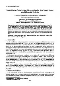
NH3 is also a pollutant and may cause severe respiratory diseases. Therefore, the main challenge of Sustainability 2016, 8, 478 2 of 13 the SCR is the control of urea injection amount to deal with the optimal trade-off problem between the NOx challenge of the SCR is the control of urea injection amount to deal with the optimal trade‐off problem conversion efficiency and NH3 slip [8]. between the NO x conversion efficiency and NH slip [8]. and methods for urea injection, including Researchers have proposed various control3strategies open-loopResearchers have proposed various control strategies and methods for urea injection, including control [9], closed-loop control [10–12] and model predictive and adaptive control [13–15]. open‐loop control [9], closed‐loop control [10–12] and model predictive and adaptive control [13–15]. Another way of dealing with this problem is the use of multi-objective genetic algorithms. The first Another way of dealing with this problem is the use of multi‐objective genetic algorithms. The first step of the proposed method is to build engine and SCR models for the prediction of the upstream step of the proposed method is to build engine and SCR models for the prediction of the upstream and downstream NOx emissions and NH3 slip to obtain the two conflicting objective functions and downstream NOx emissions and NH3 slip to obtain the two conflicting objective functions (NOx (NOxconversion conversionefficiency efficiency andNH NH forthe themulti‐objective multi-objective optimization. multi-objective 3 slip) and 3 slip) for optimization. The The multi‐objective optimization method is then used to optimize the decision variable (urea injection amount) to maximize optimization method is then used to optimize the decision variable (urea injection amount) to NOx maximize NO conversion efficiency while minimizing the NH3 slip under certain operating points. x conversion efficiency while minimizing the NH 3 slip under certain operating points. Figure 1 shows a schematic of a catalytic converter illustrating how NO Figure 1 shows a schematic of a catalytic converter illustrating how NO x emissions are converted x emissions are converted into nitrogen gas and water. Figure 1 also indicates the possible emissions of non‐reactive NH 3 (NH3 NH into nitrogen gas and water. Figure 1 also indicates the possible emissions of non-reactive 3 slip) and non‐reactive NO x . (NH3 slip) and non-reactive NOx .
Figure 1. Schematic for the conversion of NO Figure 1. Schematic for the conversion of NOx to nitrogen and water. x to nitrogen and water.
A good number of research activities have been conducted and have proposed a variety of ways
A number research activities have been conducted and have proposed a variety of for good predicting NOof x emissions [16–19]. A study [20] used artificial neural networks to build a waysprediction for predicting emissions [16–19]. Areferences study [20][19,21], used artificial neural to build a model NO for xCO 2, soot, and NOx. In an adaptive least networks squares support prediction model for CO2 , soot, and NOx . In references x[19,21], an adaptive least squares support vector machine model was built for the prediction of NO emissions with a novel update to tackle vectorprocess variations. The support vector machine (SVM), which is established based on the structural machine model was built for the prediction of NOx emissions with a novel update to tackle risk minimization proven to exhibit better generalization performance than process variations. Theprinciple, supporthas vector machine (SVM), which is established based on theneural structural networks and other methods [22]. In the work of Martinez‐Moraleset [23], artificial neural networks risk minimization principle, has proven to exhibit better generalization performance than neural were used for the non‐linear identification of a gasoline engine for the purpose of evaluating objective networks and other methods [22]. In the work of Martinez-Moraleset [23], artificial neural networks functions used within an optimization framework involving the use of the NSGA‐II genetic algorithm were used for the non-linear identification of a gasoline engine for the purpose of evaluating objective and the Multi‐Objective Particle Swarm Optimization (MOPSO) algorithm. It was observed that the functions used within an optimization framework involving the use of the NSGA-II genetic algorithm NSGA‐II algorithm performed better than the MOPSO algorithm in the Pareto based optimization and the Multi-Objective Particle Swarm Optimization (MOPSO) algorithm. It was observed that the process. In the study [24], it was found, again, that the multi‐objective optimization solution for the NSGA-II algorithm performed better than the MOPSO algorithm in the Pareto based optimization NSGA‐II algorithm was better than that of the ε‐constraint method. process. In the study [24], it was found, again, that the multi-objective optimization solution for the Against the background given above, the current study proposed a novel method based on an SVM (Support Vector Machine) and GA (Genetic algorithm) for modeling a target diesel engine and NSGA-II algorithm was better than that of the ε-constraint method. SCR system to predict upstream and downstream NO x emissions and NH 3 slip. The NSGA‐II genetic Against the background given above, the current study proposed a novel method based on algorithm was used for the multi‐objective optimization involving the maximization of NO x an SVM (Support Vector Machine) and GA (Genetic algorithm) for modeling a target diesel engine conversion efficiency while minimizing NH3 slip because it has proven to give better optimal results and SCR system to predict upstream and downstream NOx emissions and NH3 slip. The NSGA-II compared with other optimization methods as observed in references [23,24]. genetic algorithm was used for the multi-objective optimization involving the maximization of NOx conversion efficiency while minimizing NH3 slip because it has proven to give better optimal results 2. Experimental Setup and Methods compared with other optimization methods as observed in references [23,24].
As discussed in Section 1, the first step of the current study is to build prediction models for estimating engine and SCR system output as close as possible to the actual output y for an input 2. Experimental Setup and Methods vector , , ,…, using optimal SVM (support vector machine) models. The SVM is the As discussed in Section 1, the first step the current study to buildsystem prediction models most appropriate method for obtaining the of prediction model of a is stochastic from a small for
estimating engine and SCR system output yˆ as close as possible to the actual output y for an input
Sustainability 2016, 8, 478
3 of 13
vector X “ px1 , x2 , x3 , . . . , xn q using optimal SVM (support vector machine) models. The SVM is the most appropriate method for obtaining the prediction model of a stochastic system from a small amount of experimental data [25]. After obtaining the prediction models, non-dominated sorting genetic algorithm (NSGA-II) was implemented to deal with the trade-off between the two conflicting objective functions of NOx conversion efficiency and NH3 slip under certain working points. The whole procedures of modeling and multi-objective optimization were implemented in MATLAB® (MathWorks, Inc., Natick, MA, USA). 2.1. Data Collection In this study, data was collected by running a four-stroke, six-cylinder YUCHAI YC6L-42 diesel engine on a dynamometer. The main specifications of the experimental engine as well as the dynamometer and associated instrumentation are presented in Tables 1 and 2 respectively. The Eddy-current dynamometer and associated instrumentation were used in the experiments to measure engine speed and torque with the fuel supply per cycle being obtained from the CAN bus directly. The AVL 4000 and the LDS6 instrumentation were used for the measuring of NOx emissions and NH3 slip, respectively. In order to cover as many common operating points of the diesel engine as possible, 180 equally spaced operating points were selected, with speed ranging from 900 rpm to 2600 rpm (with a step size of 100 rpm) and engine load ranging from 10% to 100% (with a step size of 10%). Parts of these are shown in Table 3. Table 1. Technical specifications of the experimental engine. Features
Parameters
Engine type Number of cylinder Displacement volume Max. power Max. torque Cooling system
YUCHAI YC6L-42 6 6.6 L 179 kW 940 N¨ m Water-cooled
Table 2. The parameter measurement methods. Equipment
Measurement Parameters
Eddy current dynamometer CAN bus AVL4000 LDS6
Speed, torque circulating oil NOx emissions NH3 slip
Table 3. Engine operating conditions. Mode
Speed (rpm)
Torque (N*m)
Load (%)
Fuel Supply (mg/cyc)
Temperature of Catalyst (˝ C)
Upstream NOx (ppm)
1 2 3 4 5 6 7 8 9 10 11 12
1000 1000 1000 1500 1500 1500 2000 2000 2000 2500 2500 2500
215 391 585 204 408 612 201 395 596 153 312 471
30 60 90 30 60 90 30 60 90 30 60 90
171 309 503 168 300 436 178 299 429 165 265 364
215 326 492 250 344 415 249 318 394 227 296 378
862 1401 849 684 1131 1306 498 767 1026 290 489 674
Sustainability 2016, 8, 478
4 of 13
2.2. Data Preprocessing Generally, there are some numerical discrepancies among input variables x1 , x2 , x3 , . . . , xn , and, as a consequence, some variables may not have a significant influence on the system’s output y. Therefore, in order to eliminate the negative impact caused by the huge numerical discrepancies of input variables, there was the need to normalize each variable to vary from 0 to 1. For each column of data sample xi , the normalized data sample is given by: xi 1 “
xi ´ xi pminq xi pmaxq ´ xi pminq
(1)
where xi is the original data, xi 1 is the normalized data, and xi (max) and xi (min) are the maximum and minimum in xi , respectively. Subsequently, the normalized data xi 1 were used as the inputs for the SVM models. 2.3. Building and Optimizing the SVM Models The Support Vector Machine (SVM) [26] was developed by Vapnik and Cortes in 1995. As a novel kind of machine learning method, the SVM is gaining increasing popularity because of its many attractive features and promising empirical performance. A detailed description of SVM theory can be found in references [27–29]. Here, only a brief description is given. A support vector machine takes advantage of the kernel function to map the input data onto a high-dimensional feature space. Linear regression is then performed in the high-dimensional feature space. As a result, non-linear problems can be addressed in a linear space through non-linear feature mapping. After training on the input data sample, the SVM model can be used to predict variables whose values are unknown. The final prediction function used by an SVM is as follows: f pxq “
m ÿ
ai yi Kpxi , xq ` b
0 ă ai ă C
(2)
i “1
where ai is Lagrange multiplier, and xi is a feature vector corresponding to a training variable. The components of vector ai and the constant b are optimized during training. C is a penalty factor, which indicates the degree of attention paid to outliers and determines the range of ai . The larger the value of C is the more attention is paid to the outliers. The kernel function is represented by K pxi , xq, and is one of the most important parts of the SVM model. There are four common kinds of kernel functions. Among them, the Gaussian radial basis function kernel is most commonly used because of its effectiveness and speed in the modeling process [30]. The Gaussian function takes the form: Kpxi , xq “ expp´g ||x ´ xi ||2 q
(3)
where g is the parameter of the kernel function, which is as important as penalty factor C, with x and xi representing independent variables. 2.4. Model Parameter Optimization with Grid Search and GA Based on the preceding discussion, it is clear that the kernel function parameters C and g are considerably vital in the SVM model. The selection of parameters C and g directly influences the performance of the SVM model. Thus, it could be deduced that the performance of the SVM model lies in the choice of the kernel function parameter g and penalty factor C. In this study, a multi-algorithm combined method is proposed for optimizing the model parameters. A Genetic Algorithm (GA) [31] is a kind of optimization algorithm, which uses genetics to simulate the natural evolution process. Three basic operators of selection, crossover and mutation are used to
Sustainability 2016, 8, 478
5 of 13
generate better offspring populations in order to find exact or approximate solutions to optimization problems. GAs have been successfully used to solve a broad spectrum of optimization problems owing to its Sustainability 2016, 8, 478 high effectiveness and lower time consumption [32]. 5 of 13 Therefore, in this study, a genetic algorithm was used to optimize the C and g parameters of the SVM Therefore, in this study, a genetic algorithm was used to optimize the C and g parameters of the model. Furthermore, the k-fold cross-validated root mean squared error (RMSE) [33] was SVM Furthermore, the k‐fold cross‐validated squared error (RMSE) [33] was selected asmodel. the fitness of the objective function for the root GA mean to reflect the prediction accuracy of the SVMselected as the fitness of the objective function for the GA to reflect the prediction accuracy of the model. d řN SVM model. ˆ 2 i“1 py ´ yq RMES “ (4) N ∑ (4)
where N is the number of samples, with y and yˆ representing the actual and predicted values respectively. The main objective of the GA was to yield the smallest k-fold cross-validated RMSE by where N is the number of samples, with y and y representing the actual and predicted values searching for the best combinations of the C and g parameters for the SVM model. respectively. The main objective of the GA was to yield the smallest k‐fold cross‐validated RMSE by In a GA, prior to the initial random population generation, the ranges of each searching for the best combinations of the C and g parameters for the SVM model. parameter need to be given, In a GA, prior to the initial random population generation, the ranges of each parameter need to which are almost given empirically at present. If the ranges were too wide, the optimization be given, which are almost given empirically at present. If the ranges were too wide, the optimization process would be time-consuming. On the other hand, if the ranges were too small, the best parameters process would be On other hand, if the ranges were small, the the best may not be captured intime‐consuming. the ranges. Based onthe this, a grid search is proposed for too determining rough may Innot be captured in the ranges. Based on that this, identifying a grid search is proposed for pair scopeparameters in this study. addition, existing studies have shown a good parameter determining the rough scope in this study. In addition, existing studies have shown that identifying by searching exponentially in the sequences is more practical and less time-consuming. For example, a good parameter pair by searching exponentially in the sequences is more practical and less time‐ C = 2´2 , 2´1 , ¨ ¨ ¨ , 210 ; g = 2´1 , 20 ,−2¨ ¨ ¨ −1, 210 [34]. consuming. For example, C = 2 , 2 , ⋯, 210; g = 2−1, 20, ⋯, 210 [34]. The The procedure of optimizing the C and g parameters of the SVM with grid search and GA is procedure of optimizing the C and g parameters of the SVM with grid search and GA is shown in Figure 2 as follows: shown in Figure 2 as follows:
Figure 2. Optimizationn of Support Vector Machine (SVM) model with Genetic Algorithm (GA).
Figure 2. Optimizationn of Support Vector Machine (SVM) model with Genetic Algorithm (GA).
Step 1: Involves the use of a grid search in the range of C ∈ [2−10, 215] and g ∈ [2−5, 210]
Step 1: Involves the use of a grid search in the range of C P [2´10 , 215 ] and g P [2´5 , 210 ] according according to the exponential sequences mentioned earlier. The k‐fold cross‐validated RMSE for all to thepairs of C and g parameters is evaluated for the SVM model in the process of finding the best pair. exponential sequences mentioned earlier. The k-fold cross-validated RMSE for all pairs of C and Step 2: Based on the best pair of C and g parameters determined in Step 1, the ranges of each g parameters is evaluated for the SVM model in the process of finding the best pair. parameter in the GA are established. Subsequently, a two‐dimensional random initial population, Step 2: Based on the best pair of C and g parameters determined in Step 1, the ranges of each which is binary encoded, is created. Each dimension (chromosome) represents C and g, respectively. parameter in the GA are established. Subsequently, a two-dimensional random initial population, Step 3: Involves the calculation of the fitness function of all populations given by the k‐fold cross‐ which is binary encoded, is created. Each dimension (chromosome) represents C and g, respectively. validated RMSE for the SVM model. Step 3: Involves the calculation of the fitness function of all populations given by the k-fold Step 4: Based on fitness level (k‐fold cross‐validated RMSE), a better offspring population is cross-validated RMSE for the SVM model. generated through the use of the three basic genetic operators of selection, crossover and mutation. Step 4: Based on fitness level (k-fold cross-validated RMSE), a better offspring population is In this study, the probabilities for the selection, crossover and mutation operators were set to 0.9, 0.8 generated through the use of the three basic genetic operators of selection, crossover and mutation. and 0.05, respectively. Step the 5: In this step, Step was selection, repeated until the stopping criterion (100 generations for In this study, probabilities for4 the crossover and mutation operators were set tothe 0.9, 0.8 current study) was satisfied. and 0.05, respectively.
Sustainability 2016, 8, 478
6 of 13
Step 5: In this step, Step 4 was repeated until the stopping criterion (100 generations for the current study) was satisfied. After these steps, the best pair of C and g was obtained, ending the optimization process for the SVM models. 2.5. Multi-Objective Optimization After building and optimizing the three prediction models for the upstream and downstream NOx emissions as well as NH3 slip, the ultimate goal of this study was to optimize the urea injection amount to maximize the NOx conversion efficiency while minimizing the NH3 slip, a situation that characterizes a typical multi-objective optimization problem. A multi-objective optimization problem is usually concerned with maximizing or minimizing a number of objective functions in the presence of certain inequality and equality constraints, as well as other constraints in the form of lower and upper bounds defining the decision variable space. Generally, multi-objective optimization problems do not have a single optimal solution but a Pareto optimal set for the conflict between the various goals, and, as a consequence, it is therefore virtually impossible for multiple objectives to simultaneously achieve optimal results. The NSGA-II genetic algorithm was proposed by Kalyanmoy et al. [35] to help reduce the computational complexity based on a certain number of decision variables and a given population of solutions, preserve the elite members of a population of solutions and eliminate the need for a sharing parameter associated with other multi-objective evolutionary algorithms like the Pareto-archived evolutionary strategy (PAES) [36] and the strength-Pareto evolutionary algorithm (SPEA) [37]. NSGA-II takes advantage of the non-dominated sorting and crowding distance so that the algorithm has the capacity to approximate the best Pareto frontier and ensure that the obtained Pareto optimal solution has a good spreading. The specific description of the NSGA-II can be found in references [35,38,39]. The basic procedure for executing NSGA-II for the current multi-objective problem is summarized in Figure 3 and the steps are as follows: Step 1: Involves fixing the parameters and the range of the decision variable (urea injection amount). In the current study, an initial solutions population of 100 and a maximum number of generations of 200 were used for the multi-objective optimization. The lower and upper bounds for the urea injection amount variable were 0 and 2000 mL/h, respectively. Step 2: Based on the parameters and ranges determined in Step 1, a random initial population, which is binary encoded, was created. Step 3: Involves the calculation of the ranks and crowding distance of the population, followed by the application of the tournament selection method for selecting the best solutions in a particular population for creating a mating pool for producing child solutions based on non-dominated sorting. Step 4: Involves the generation of offspring and parent population through crossover and mutation operators to ensure that the diversity within different generations of solutions is preserved. The best individuals were selected as the new population from the population incorporating offspring and parent population based on non-dominated sorting. In this study, probabilities of 0.9 and 0.1 were used for the crossover and mutation operators for the multi-optimization framework, respectively. Step 5: In this step, a repetition of Step 3 and Step 4 was carried out until the stopping criterion (200 generations for the current study) was satisfied. After these steps, the optimal Pareto set of the decision variable (urea injection amount) was obtained.
Sustainability 2016, 8, 478 Sustainability 2016, 8, 478 Sustainability 2016, 8, 478
7 of 13 7 of 13 7 of 13
Figure 3. General procedure for executing the Non‐dominated Sorting Genetic Algorithm (NSGA‐II) Figure 3. General procedure for executing the Non-dominated Sorting Genetic Algorithm (NSGA-II) Figure 3. General procedure for executing the Non‐dominated Sorting Genetic Algorithm (NSGA‐II) multi‐objective optimization in the current study. multi-objective optimization in the current study. multi‐objective optimization in the current study.
3. Results and Discussion 3. Results and Discussion 3. Results and Discussion 3.1. Results for SVM Model Simulation 3.1. Results for SVM Model Simulation 3.1. Results for SVM Model Simulation Based on the the modeling modeling and optimization methods discussed in Section three prediction Based on and optimization methods discussed in Section 2, three2, models Based on the modeling and optimization methods discussed in Section 2, prediction three prediction models were obtained. One was an engine model for predicting upstream NO x emissions. The other were obtained. One was an engine model for predicting upstream NOx emissions. The other two were models were obtained. One was an engine model for predicting upstream NO x emissions. The other two were an SCR model for predicting downstream NO x emissions and another for NH3 slip under an SCR model for predicting downstream NO emissions and another for NH slip under different x 3 two were an SCR model for predicting downstream NO x emissions and another for NH 3 slip under different operating points. Half (1/2) of the equally spaced data samples were selected as the training operating points. Half (1/2) of the equally spaced data samples were selected as the training dataset different operating points. Half (1/2) of the equally spaced data samples were selected as the training dataset these SVM optimal SVM After models. the models were trained, the rest 1/2 samples were for thesefor optimal models. theAfter models were trained, the rest 1/2 samples were applied to dataset for these optimal SVM models. After the models were trained, the rest 1/2 samples were applied to the model to test the generalization ability of the optimal models. The flow chart for the model to test the generalization ability of the optimal models. The flow chart for designing the applied to the model to test the generalization ability of the optimal models. The flow chart for designing the optimal SVM models is shown in Figure 4. optimal SVM models is shown in Figure 4. designing the optimal SVM models is shown in Figure 4.
Figure 4. Processes for designing the proposed SVM models. Figure 4. Processes for designing the proposed SVM models. Figure 4. Processes for designing the proposed SVM models.
Figure 5a shows shows comparison between the actual outputs and prediction model prediction for the Figure 5a thethe comparison between the actual outputs and model for the upstream Figure 5a shows the comparison between the actual outputs and model prediction for the upstream NO x emissions. Figure 5b also shows the quality of fit between the actual outputs and the NOx emissions. Figure 5b also shows the quality of fit between the actual outputs and the model upstream NO x emissions. Figure 5b also shows the quality of fit between the actual outputs and the model prediction. It is evident from Figure 5a that the curves for actual and predicted values almost prediction. It is evident from Figure 5a that the curves for actual and predicted values almost coincide, model prediction. It is evident from Figure 5a that the curves for actual and predicted values almost coincide, and the errors between them are considerably small. It can also be seen from Figure 5b that and the errors between them are considerably small. It can also be seen from Figure 5b that all the coincide, and the errors between them are considerably small. It can also be seen from Figure 5b that all the are points are evenly distributed along line the where the predicted values tracked the values actual points evenly distributed along the linethe where predicted values tracked the actual all the points are evenly distributed along the line where the predicted values tracked the actual values fairly well, implying that the upstream NO x emissions were predicted with good accuracy for fairly well, implying that the upstream NOx emissions were predicted with good accuracy for all values fairly well, implying that the upstream NO x emissions were predicted with good accuracy for all samples. Similar statistics are shown graphically for the downstream NO x emissions and NH 3 slip samples. Similar statistics are shown graphically for the downstream NOx emissions and NH3 slip in all samples. Similar statistics are shown graphically for the downstream NOx emissions and NH 3 slip in Figures 6 and 7, which also show good prediction accuracy. Figures 6 and 7 which also show good prediction accuracy. in Figures 6 and 7, which also show good prediction accuracy.
Sustainability 2016, 8, 478
8 of 13
Sustainability 2016, 8, 478 Sustainability 2016, 8, 478 1600 Sustainability 2016, 8, 478
-200
20 0
0
40
20 20
60
40 40
60 60
80
100
8 of 13 8 of 13 8 of 13
actual value predicted value actual value error predicted actual valuevalue error predicted value error
a)
-6 -6 Upstream ) NOX emissions(×10 Upstream ) NOX emissions(×10 Upstream NOX emissions(×10-6)
1600 1400 1600 1400 1200 1400 1200 1000 1200 1000 800 1000 800 600 800 600 400 600 400 200 400 200 0 200 0 -200 00 -200
a) a)
120
140
160
Sample 80 100 120 140 160 80 Sample 100 120 140 160 Sample
180 180 180
(a) (b) (a) (b) (b) NOx emissions. (a) Figure 5. Comparison (a) between experimental and predicted values for upstream Figure 5. Comparison between experimental and predicted values for upstream NO emissions.
x Figureversus 5. Comparison between experimental and predicted values for upstream NOx emissions. (a) Actual predicted output; (b) Quality of fit. (a) Actual versus predicted output; (b) Quality of fit. Figure 5. Comparison between experimental and predicted values for upstream NO x emissions. (a) Actual versus predicted output; (b) Quality of fit. a) Actual versus predicted output; (b) Quality of fit. 1000 a) 1000
actual value predicted value actual value error predicted actual valuevalue error predicted value error
a)
-6 -6 Downstream ) NOX emissions(×10 Downstream ) NOX emissions(×10 Downstream NOX emissions(×10-6)
1000 800 800 800 600 600 600 400 400 400 200 200 200 0 0 0 -200
0 -200
-200
20 0
0
20 20
40 40 40
60 60 60
80
100
120
140
160
Sample 80 100 120 140 160 80 Sample 100 120 140 160 Sample
180 180 180
(a) (b) (a) (b) (a) between experimental and predicted values for downstream (b) Figure 6. Comparison NOx emissions. Figure 6. Comparison Comparison between experimental and predicted values values for for downstream downstream NO NOx emissions. emissions. (a) Actual versus predicted output; (b) Qualityand of fit. Figure 6. between experimental predicted x Figure 6. Comparison between experimental and predicted values for downstream NO x emissions. (a) Actual Actualversus versuspredicted predicted output;(b) (b)Quality Qualityof offit. fit. b) a) (a) output; 80 (a)80 Actual versus predicted output; (b) Quality of fit. b) a) y=x actual value
-10
0
80 70 80 70 60 70
a)
data y=x fitdata y=x fit data
Predictied value ofvalue NH3of leakage(ppm) Predictied NH3 leakage(ppm) Predictied value of NH3 leakage(ppm)
predicted value actual value error predicted actual valuevalue error predicted value error
NH3 leakage(ppm) NH3 leakage(ppm) NH3 leakage(ppm)
80 70 80 70 60 70 60 50 60 50 40 50 40 30 40 30 20 30 20 10 20 10 0 10 0 -10 00 -10
b)
fit
60 50 60 50 40 50 40 30 40 30 20 30
20 0
20 20
40 40 40
60 60 60
80
100
120
140
160
Sample 80 100 120 140 160 80 Sample 100 120 140 160 Sample
180 180 180
20 10 20 10 100 0 0 0
0
10 0
20
30
40
50
60
70
Experimental value of40NH3 leakage(ppm) 20 30 50 60 70 Experimental 10 20 30 value40of NH350leakage(ppm) 60 70 Experimental value of NH3 leakage(ppm) 10
(a) (b) (a) (b) (a) between experimental and predicted values for NH (b)3 slip. (a) Actual versus Figure 7. Comparison Figure 7. output; Comparison between predicted (b) Quality of fitexperimental and predicted values for NH3 slip. (a) Actual versus Figure 7. between predicted output; (b) Quality ofexperimental fit Figure 7. Comparison Comparison between experimentaland andpredicted predictedvalues valuesfor forNH NH3 3slip. slip.(a) (a)Actual Actualversus versus predicted output; (b) Quality of fit 2 predicted output; (b) Quality of fit.
80 80 80
The RMSE (root mean square error), MAPE (mean absolute percent error) and R (correlation 2 The RMSE mean square error), MAPE (meanare absolute coefficient) values(root as well as the fits of the three models given inpercent Table 4.error) and R2 (correlation The RMSE (root mean square error), MAPE (mean absolute percent error) and R (correlation coefficient) values as well the fitserror), of the MAPE three models given percent in Tableerror) 4. The RMSE (root meanassquare (mean are absolute and R2 (correlation coefficient) values as well as the fits of the three models are given in Table 4. coefficient) values as well as the fits of the three models are given in Table 4.
Sustainability 2016, 8, 478
9 of 13
Table 4. The fit statistics for the three prediction models.
Model
Upstream NOx Emissions Training
RMSE(ppm) MAPE(%) R2 Fits
Test
Downstream NOx Emissions
All
Training
24.62 57.16 44.01 1.71 4.77 3.24 0.99 0.98 0.99 Y1 = 0.9849 ˆ X1 + 8.0395
Test
All
19.56 25.87 21.87 2.17 6.89 4.53 0.99 0.98 0.99 Y2 = 0.9644 ˆ X2 + 6.8769
NH3 Slip Training
Test
All
1.34 2.84 2.22 0.99 0.97 0.98 Y3 = 0.9786 ˆ X3 + 0.9270
The MAPE for the upstream and downstream NOx emission prediction models were under 5% for all datasets except for the test dataset for the downstream NOx emissions, which were considered good enough for estimating the outputs. It was meaningless to calculate the MAPE for the NH3 slip for the reason that the actual value of NH3 slip may be 0 for certain particular working points, and the MAPE may not be defined mathematically (that is a constant divided by 0 cannot be defined mathematically). For example, it is difficult to achieve catalytic reduction when the temperature of SCR catalyst is under 200 ˝ C. Under such a condition the urea injection amount is 0 and there is no NH3 slip. The RMES for three models of upstream NOx emissions, downstream NOx emissions and NH3 slip were 44.01 ˆ 10´6 , 21.87 ˆ 10´6 and 2.22 ˆ 10´6 respectively, which were considerably small, while the squared correlation coefficients for the three models were 0.99, 0.99 and 0.98 respectively. This implied that the accuracies of the three models were good enough for the prediction of the upstream and downstream NOx emissions and NH3 slip. The quality of fit between actual values and prediction values for the three models are also shown in Table 4. It can be also seen from Table 4 that the RMES and MAPE for the test datasets are a little larger than for the training datasets. The main reasons for this are as follows: Firstly, it was impossible to cover all the operating points of the diesel engine when choosing the training datasets for the model, which had a negative impact on the prediction accuracy. Secondly, some subjective factors existed in the parameter selection and data processing. Thirdly, there could be some outliers from such a large experimental data. Furthermore, there was no absolute guarantee that the experimental data would to be obtained in a completely steady state, and could lead to prediction errors as a consequence. 3.2. NSGA-II Multi-Objective Optimization Results The prediction models for upstream NOx emissions, downstream NOx emissions and NH3 slip are coded M1, M2 and M3, respectively, and are shown together with the inputs and outputs of the three models in Table 5. Table 5. The inputs and outputs of the three prediction models. Model
Inputs
Outputs
M1
Speed, Torque, Fuel supply pre cycle
Upstream NOx emissions
M2
Temperature, Upstream NOx emissions, urea injection amount
Downstream NOx emissions
M3
Temperature, Upstream NOx emissions, urea injection amount
NH3 slip
Equations (5) and (6) were used as objective functions for the optimization framework using the NSGA-II genetic algorithm, with Equations (7) and (8) as inequality constraints. The aim of the current research was to maximize Yε (NOx conversion efficiency) while minimizing the YNH3 (NH3 slip) using the NSGA-II genetic algorithm for the multi-objective optimization procedure discussed in Section 3. Yε “ pM1 ´ M2q{M1
(5)
YNH3 “ M3
(6)
Sustainability 2016, 8, 478
10 of 13
S.T M2 ě 0
(7)
M3 ě 0
(8)
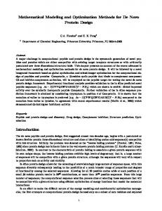
whereSustainability 2016, 8, 478 YNH3 = the NH3 slip (ppm); Yε = NOx conversion efficiency (%); and M1, M2 and M310 of 13 represent the outputs of the three models, respectively. M3 ≥ 0 To observe how the whole process functions, mode 4 in Table 3 was taken as an example,(8) and the optimization was run and terminated after 200 iterations. Under certain operating speed, torque, where YNH3 = the NH3 slip (ppm); Yε = NOx conversion efficiency (%); and M1, M2 and M3 represent fuel supply, temperature and upstream NOx emissions were fixed. The only decision variable that could be the outputs of the three models, respectively. To observe how the whole process functions, mode 4 in Table 3 was taken as an example, and changed by the researcher to deal with the trade-off between Yε (NOx conversion efficiency) and YNH3 (NH3the optimization was run and terminated after 200 iterations. Under certain operating speed, torque, slip) was the urea injection amount. Figure 8 shows the final 100 Pareto optimal solutions for fuel supply, temperature and upstream NO x emissions were fixed. The only decision variable that the objective functions Yε (NOx conversion efficiency) and YNH3 (NH3 slip), and their corresponding could be changed by the researcher to deal with the trade‐off between Yε (NOx conversion efficiency) decision variables (urea injection amount) used for the multi-objective optimization. It could be and YNH3 (NH3 slip) was the urea injection amount. Figure 8 shows the final 100 Pareto optimal seen from the graph that it is not possible to improve (increase) NOx conversion efficiency without solutions for the objective functions Yε (NOx conversion efficiency) and YNH3 (NH3 slip), and their worsening (increasing) NH3 slip. This trend generally characterizes a conflicting multi-objective corresponding decision variables (urea injection amount) used for the multi‐objective optimization. optimization problem. It could be seen from the graph that it is not possible to improve (increase) NO x conversion efficiency Among the 100 Pareto optimalNH solutions, in trend the initial stages there was a a conflicting rapid increase without worsening (increasing) 3 slip. This generally characterizes multi‐in the NOx objective optimization problem. conversion efficiency with the increase of the urea injection amount, while the value for NH3 Among the 100 Pareto optimal solutions, in the initial stages there was a rapid increase in the slip increased slightly. On the other hand, the NOx conversion efficiency gradually decreased, while NO x conversion efficiency with the increase of the urea injection amount, while the value for NH the rate of NH3 slip gradually increased. Finally, NH3 slip goes up rapidly with the increase of3 urea slip increased slightly. On the other hand, the NO x conversion efficiency gradually decreased, while injection amount, while the NOx conversion efficiency remains constant at 0.95. the rate of NH3 slip gradually increased. Finally, NH3 slip goes up rapidly with the increase of urea For this particular multi-objective optimization problem, related emissions legislation (WHTC for injection amount, while the NOx conversion efficiency remains constant at 0.95. Euro VI) requires that the real-time value of NH3 slip should be less than 10 ppm. Therefore, a vertical For this particular multi‐objective optimization problem, related emissions legislation (WHTC line was drawn through the 10 ppm point on the horizontal axis, with the two points A(9.7, 0.88) and for Euro VI) requires that the real‐time value of NH 3 slip should be less than 10 ppm. Therefore, a B(9.7,vertical line was drawn through the 10 ppm point on the horizontal axis, with the two points A(9.7, 940) which are closest to the left of vertical line (NH3 slip less than 10 ppm) on the curves for the Pareto optimal frontier and the urea injection amount were taken as the optimal solution for the 0.88) and B(9.7, 940) which are closest to the left of vertical line (NH 3 slip less than 10 ppm) on the multi-objective problem operating mode 4.urea injection amount were taken as the optimal curves for the Pareto under optimal frontier and the solution for the multi‐objective problem under operating mode 4. Point A represents the final optimal solution for the multi-objective optimization problem and point B isPoint A represents the final optimal solution for the multi‐objective optimization problem and the corresponding urea injection amount under operating mode 4. In other words, for modepoint B is the corresponding urea injection amount under operating mode 4. In other words, for mode 4, with an upstream NOx concentration of 684 ppm and a catalytic converter temperature of 4, with an upstream NOx concentration of 684 ppm and a catalytic converter temperature of 250 °C, 250 ˝ C, the optimal amount of urea which results in the optimal performance of the SCR catalytic the optimal amount of urea which results in the optimal performance of the SCR catalytic converter converter (88% reduction of NOx emissions and 9.7 ppm NH3 slip) is 940 mL/h. Similar results for (88% reduction of NOx emissions and 9.7 ppm NH3 slip) is 940 mL/h. Similar results for other working otherconditions working can conditions can also using be achieved theThe same method. The optimization results also be achieved the same using method. optimization results for modes 4–9 for modes 4–9 (engine speed = 1500 rpm and 2000 rmp) of Table 3 are summarized and presented (engine speed = 1500 rpm and 2000 rmp) of Table 3 are summarized and presented in Table 6. The in Table 6. The designer can also obtain other optimal solutions to the multi-objective optimization designer can also obtain other optimal solutions to the multi‐objective optimization problem from problem from the Pareto front by setting other restrictions in the form of constraints. the Pareto front by setting other restrictions in the form of constraints. Pareto front 1
1500
Pareto optimal solutions Urea injection amount
0.9
1350 1200
A
0.7
1050
0.6
900
0.5
750
B 0.4
600
0.3
450
0.2
300
0.1
150
0
0
2
4
6 8 10 12 YNH3(NH3 leakage(ppm))
14
16
Urea injection amount(mL/h)
Yε(NOX conversion efficiency(%)
0.8
0 18
Figure 8. Pareto‐based optimal solutions to the multi‐objective optimization problem. Figure 8. Pareto-based optimal solutions to the multi-objective optimization problem.
Sustainability 2016, 8, 478
11 of 13
Table 6. Optimization results for the engine speeds of 1500 rpm and 2000 rpm. Model
Speed (rpm)
Torque (N*m)
Temperature ˝C
Upstream NOx (ppm)
Urea Injection Amount (mL/h)
NOx Conversion Efficiency (%)
NH3 Slip (ppm)
4 5 6 7 8 9
1500 1500 1500 2000 2000 2000
204 408 612 201 395 596
250 344 415 249 318 394
684 1131 1306 498 767 1026
940 1256 1553 698 1468 1178
88 90 90 91 87 92
9.7 9.8 9.6 9.4 9.6 9.3
4. Conclusions A novel ensemble methodology with GA and SVM has been presented for establishing the models for the prediction of upstream and downstream NOx emissions and the NH3 slip. The various aspects of the modeling and optimization processes have been discussed in detail. The NSGA-II was used to solve the multi-objective optimization problem of maximizing NOx conversion efficiency while minimizing NH3 slip based on the decision variable of urea injection amount under certain operating points. Based on the current study, the following conclusions could be drawn: (1)
(2)
The prediction accuracy of the engine and SCR models could be improved by using an SVM, the parameters of which were optimized using a GA. The RMSE of upstream and downstream NOx emissions and NH3 slip for the all datasets was 44.01 ˆ 10´6 , 21.87 ˆ 10´6 and 2.22 ˆ 10´6 , respectively. The MAPE of the models were all under 5%, and was good enough for estimating the actual outputs. The optimized urea injection amounts under certain operating points were obtained through multi-objective genetic algorithm for maximizing NOx conversion efficiency while minimizing NH3 slip.
Acknowledgments: The authors would like to express their deep appreciation to the Hubei Key Laboratory of Advanced Technology for Automotive Components (Wuhan University of Technology). The authors also wish to extend their appreciation to the National Natural Science Foundation of China (Grant No. 51406140) for financially supporting the study. Author Contributions: All authors have contributed equally to the design of the research, data collection and analysis and the final preparation of the manuscript. Conflicts of Interest: The authors declare no potential conflict of interest.
References 1.
2. 3. 4. 5. 6.
7.
Brookshear, D.W.; Nguyen, K.; Toops, T.J.; Bunting, B.G.; Rohr, W.F. Impact of Biodiesel-Based Na on the Selective Catalytic Reduction of NOx by NH3 over Cu–Zeolite Catalysts. Top. Catal. 2013, 56, 62–67. [CrossRef] Chen, P.; Wang, J. Nonlinear and adaptive control of NO/NO2 ratio for improving selective catalytic reduction system performance. J. Eng. Marit. Environ. 2007, 221, 31–42. [CrossRef] Iwasaki, M.; Shinjoh, H. A comparative study of “standard”, “fast” and “NO2 ” SCR reactions over Fe/zeolite catalyst. Appl. Catal. A Gen. 2010, 390, 71–77. [CrossRef] Forzatti, P. Present status and perspectives in de-NOx SCR catalysis. Appl. Catal. A Gen. 2001, 222, 221–236. [CrossRef] Koebel, M.; Elsener, M.; Madia, G. Recent Advances in the Development of Urea-SCR for Automotive Applications; SAE International: Warrendale, PA, USA, 2001. Majd, E.; Shamekhi, A.H. Development of a neural network model for selective catalytic reduction (SCR) catalytic converter and ammonia dosing optimization using multi objective genetic. Chem. Eng. J. 2010, 165, 508–516. Beale, A.M.; Lezcano-Gonzalez, I.; Maunula, T.; Palgrave, R.G. Development and characterization of thermally stable supported V–W–TiO2 catalysts for mobile NH3 –SCR applications. Catal. Struct. React. 2015, 1, 25–34. [CrossRef]
Sustainability 2016, 8, 478
8. 9.
10. 11. 12. 13. 14.
15. 16. 17. 18.
19. 20.
21. 22. 23.
24. 25. 26. 27. 28. 29. 30. 31. 32.
12 of 13
Karimi, H.R.; Zhang, H.; Zhang, X.; Wang, J.; Chadli, M. Control and Estimation of Electrified Vehicles. J. Frankl. Inst. 2015, 352, 421–424. [CrossRef] Ardanese, R.; Ardanese, M.; Besch, M.C.; Adams, T.; Thiruvengadam, A.; Shade, B.C.; Gautam, M.; Oshinuga, A.; Miyasato, M. Development of an Open Loop Fuzzy Logic Urea Dosage Controller for Use with an SCR Equipped HDD Engine. In Proceedings of ASME 2009 Internal Combustion Engine Division Fall Technical Conference, Lucerne, Switzerland, 27–30 September 2009; pp. 353–363. Hu, J.; Zhao, Y.; Zhang, Y.; Shuai, S. Development of Closed-Loop Control Strategy for Urea-SCR Based on NOx Sensors; SAE Technical Paper; SAE International: Warrendale, PA, USA, 2011. Willems, F.; Cloudt, R. Experimental demonstration of a new model-based SCR control strategy for cleaner heavy-duty diesel engines. IEEE Trans. Control Syst. Technol. 2011, 19, 1305–1313. [CrossRef] Willems, F.; Cloudt, R.; van den Eijnden, E.; van Genderen, M. Is Closed-Loop SCR Control Required to Meet Future Emission Targets?; SAE International: Warrendale, PA, USA, 2007. Herman, A.; Wu, M.; Cabush, D.; Shost, M. Model based control of SCR dosing and OBD strategies with feedback from NH3 sensors. SAE Int. J. Fuels Lubr. 2009, 2, 375–385. [CrossRef] Zambrano, D.; Tayamon, S.; Carlsson, B.; Wigren, T. Identification of a discrete-time nonlinear Hammerstein-Wiener model for a selective catalytic reduction system. In Proceedings of the American Control Conference (ACC), San Francisco, CA, USA, 29 June–1 July 2011. Surenahalli, H.S.; Parker, G.; Johnson, J.H. Extended Kalman Filter Estimator for NH3 Storage, NO, NO2 and NH3 Estimation in a SCR; SAE Technical Paper; SAE International: Warrendale, PA, USA, 2013. D Ambrosio, S.; Finesso, R.; Fu, L.; Mittica, A.; Spessa, E. A control-oriented real-time semi-empirical model for the prediction of NOx emissions in diesel engines. Appl. Energy 2014, 130, 265–279. [CrossRef] Asprion, J.; Chinellato, O.; Guzzella, L. A fast and accurate physics-based model for the NOx emissions of Diesel engines. Appl. Energy 2013, 103, 221–233. [CrossRef] Maroteaux, F.; Saad, C. Combined mean value engine model and crank angle resolved in-cylinder modeling with NOx emissions model for real-time Diesel engine simulations at high engine speed. Energy 2015, 88, 515–527. [CrossRef] Lv, Y.; Yang, T.; Liu, J. An adaptive least squares support vector machine model with a novel update for NOx emission prediction. Chemom. Intell. Lab. Syst. 2015, 145, 103–113. [CrossRef] Taghavifar, H.; Mardanib, A.; Mohebbib, A.; Khalilaryaa, S.; Jafarmadara, S. Appraisal of artificial neural networks to the emission analysis and prediction of CO2 , soot, and NOx of n-heptane fueled engine. J. Clean. Prod. 2016, 112, 1729–1739. [CrossRef] Lv, Y.; Liu, J.; Yang, T.; Zeng, D. A novel least squares support vector machine ensemble model for NOx emission prediction of a coal-fired boiler. Energy 2013, 55, 319–329. [CrossRef] Vapnik, V.N.; Vapnik, V. Statistical Learning Theory; Wiley New York: New York, NY, USA, 1998; Volume 1. Martínez-Morales, J.D.; Palacios-Hernández, E.R.; Velázquez-Carrillo, G.A. Modeling and multi-objective optimization of a gasoline engine using neural networks and evolutionary algorithms. J. Zhejiang Univ. Sci. A 2013, 14, 657–670. [CrossRef] D Errico, G.; Cerri, T.; Pertusi, G. Multi-objective optimization of internal combustion engine by means of 1D fluid-dynamic models. Appl. Energy 2011, 88, 767–777. [CrossRef] Shin, K.; Lee, T.S.; Kim, H. An application of support vector machines in bankruptcy prediction model. Expert Syst. Appl. 2005, 28, 127–135. [CrossRef] Vapnik, V.N. The Nature of Statistical Learning Theory. IEEE Trans. Neural Netw. 1995, 10, 988–999. [CrossRef] [PubMed] Severyn, A.; Moschitti, A. Large-Scale Support Vector Learning with Structural Kernels. Lect. Notes Comput. Sci. 2010, 6323, 229–244. Tong, H.; Chen, D.R.; Yang, F. Learning Rates for -Regularized Kernel Classifiers. J. Appl. Math. 2013, 2013, 1–11. [CrossRef] Dibike, Y.B.; Velickov, S.; Solomatine, D.; Abbott, M. Model Induction with Support Vector Machines: Introduction and Applications. J. Comput. Civ. Eng. 2001, 15, 208–216. [CrossRef] Smola, A.J. Learning with kernels | Support Vector Machines. Lect. Notes Comput. Sci. 2008, 42, 1–28. Goldberg, D.E. Genetic Algorithms in Search Optimization and Machine Learning; Addison-Wesley Professional: Boston, MA, USA, 1989; Volume 412. Goldberg, D.E. Genetic Algorithms; Pearson Education: Upper Saddle River, NJ, USA, 2006.
Sustainability 2016, 8, 478
33.
34.
35. 36.
37. 38. 39.
13 of 13
Chen, R.; Sun, D.-Y.; Qin, D.-T.; Luo, Y.; Hu, F.-B. A novel engine identification model based on support vector machine and analysis of precision-influencing factors. J. Cent. South Univ.: Sci. Technol. 2010, 41, 1391–1397. Zhou, H.; Zhao, J.P.; Zheng, L.G.; Wang, C.L.; Cen, K.F. Modeling NOx emissions from coal-fired utility boilers using support vector regression with ant colony optimization. Eng. Appl. Artif. Intell. 2012, 25, 147–158. [CrossRef] Deb, K. Multi-Objective Optimization Using Evolutionary Algorithms; John Wiley & Sons: New York, NY, USA, 2001; Volume 16. Knowles, J.; Corne, D. The pareto archived evolution strategy: A new baseline algorithm for pareto multiobjective optimization. In Proceedings of the 1999 Congress on Evolutionary Computation, 1999, Washington, DC, USA, 6–9 July 1999. Zitzler, E. Evolutionary Algorithms for Multiobjective Optimization: Methods and Applications; ETH Zurich: Zürich, Switzerland, 1999. Coello, C.A.; Christiansen, A.D. Multiobjective optimization of trusses using genetic algorithms. Comput. Struct. 2000, 75, 647–660. [CrossRef] Osyczka, A. Multicriteria optimization for engineering design. Des. Opt. 1985, 1, 193–227. © 2016 by the authors; licensee MDPI, Basel, Switzerland. This article is an open access article distributed under the terms and conditions of the Creative Commons Attribution (CC-BY) license (http://creativecommons.org/licenses/by/4.0/).