@INPROCEEDINGS{correlldars04, AUTHOR = {N. Correll and A. Martinoli}, TITLE = {Modeling and Optimization of a Swarm-Intelligent Inspection System}, BOOKTITLE = {Proceedings of the 7th Symposium on Distributed Autonomous Robotic System (DARS)}, YEAR = {2004}, PUBLISHER = { Toulouse. Distributed Autonomous Systems 6. To Appear}, }
Modeling and Optimization of a Swarm-Intelligent Inspection System Nikolaus Correll and Alcherio Martinoli Swarm-Intelligent Systems Group, Nonlinear Systems Laboratory, EPFL CH-1015 Lausanne, Switzerland nikolaus.correll|
[email protected]
Abstract We present a simple, behavior-based, distributed control algorithm to inspect a regular structure with a swarm of autonomous, miniature robots, using only on-board, local sensors. To estimate intrinsic advantages and limitations of the proposed control solution, we capture its characteristics at a higher abstraction level using non-spatial probabilistic microscopic and macroscopic models. Both models achieve consistent prediction on the chosen swarm metric and deliver a series of interesting qualitative and quantitative insights on further, counterintuitive, improvement of the distributed control algorithm. Modeling results were validated by experiments with one to twenty robots using a realistic simulator in the framework of a case study concerned with the inspection of a jet turbine.
1 Introduction In order to minimize failure of jet turbine engines, the engines have to be inspected at regular intervals. This is usually performed visually using borescopes, a process which is time consuming and cost intensive [5]. One possible solution to speed up and automatize the inspection process is to rely on a swarm of autonomous, miniature robots which could be sent into the turbine without disassembling it. While this idea is intellectually appealing and could pave the way for other similar applications in coverage/inspection of engineered or natural, regular structures, it involves a series of technical challenges which dramatically limit possible designs of robotic sensors. For instance, the shielded, complex, and narrow structure of a turbine imposes not only strong miniaturization constraints on the design, but also prevents the use of any traditional global positioning and communication system. Furthermore, a limited on-board energy budget might prevent computation of a sophisticated deliberative planning strategy and dramatically narrows sensor and communication range of our robots [3]. In this paper, we perform a series of simplifications to the turbine inspection
2
Nikolaus Correll and Alcherio Martinoli
scenario and present one of the simplest algorithms for such a task. The robots have local, on-board sensors and a simple behavior-based controller that allows them to avoid collisions, follow a blade contour (emulating inspection for blade flaws), and move from blade to blade by exploiting the regularity of the turbine pattern and specific features of the blades (e.g., tips). Similar to previous case studies concerned with distributed manipulation of objects (see for instance [1, 6]), we make use of non-spatial probabilistic microscopic and macroscopic models in order to understand general properties of the inspection (or coverage) problem, and to estimate and optimize performance and reliability of our approach.
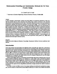
2 The Case Study: Turbine Inspection In this paper, we are not concerned with the reliable detection of flaws and progress reporting but rather with individual and group motion in the turbine scenario. For the sake of simplicity, we therefore assume that completely circumnavigating a blade is a good emulation of the scanning-for-flaws maneuver. 2.1 Simplification and Simulation of the Turbine Scenario Figure 1, left shows the simulated scenario for this case study. We simplify the real 3D environment by unrolling the axis-symmetric geometry of the turbine into a flat representation with the blades as vertical extrusions. The resulting rectangular arena (246 × 186cm2 ) is delimited by walls (emulating the boundaries of the compressor section) on the short edges and a “wraparound” zone (emulating the continuity of the turbine cylinder) on the long edge.
0.08
0.06
0.04
0.02
0
−0.02
−0.04
−0.12
−0.1
−0.08
−0.06
−0.04
−0.02
0
0.02
0.04
Fig. 1. Left: Overview of the turbine set-up in the embodied simulator. Middle: Close-up of blades and robots. Right: Interaction between a static robot (center) and a moving one. Dots correspond to positions at which the static robot was detected by the moving robot. The corresponding average detection area is indicated by a circle.
Swarm-Intelligent Inspection System
3
We implemented this simplified turbine environment using Webots 4.0 [7], a realistic, multi-robot, embodied, sensor-based simulator. In Webots, simulated sensors and actuators are characterized by precise, user-definable nonlinearities and noise—in our simulations, all sensors and actuators on-board are characterized by ±10 percent white noise. As shown in previous publications, this simulator can provide realistic results (e.g. [1, 6]) when compared with real robot experiments. It is worth noting that to allow comparison with real robotic experiments [3], we limit the simulated experimental setup to 16 blades in four stages, and the maximum number of robots to 20. 2.2 The Behavior-Based Robot Controller The behavior of a single robot is determined by a schema-based controller [2] that tightly links the platform’s actions to sensor perception while using as little representational knowledge of the world as possible. For a schema-based controller, behavioral responses are represented by vectors generated from local potential fields, and behavioral coordination is achieved by vector addition. Sequencing of behaviors is achieved by a dynamic action-selection mechanism based on two internal timers which are set and reset by the schemas. The overall behavior of a robot can be summarized as follows (see Figure 2, PFSM
FSM
k)
i( p bM
Blade Circle Blade
Search
Search
Finished Obstacle
Avoided
Avoid Collision
pr(N0-1) Avoid robot
Trobot
Ns
Circle insp. Blade
Virgin Blades
Mv
xD (k-Tb )
pb M v (k
)
pw Avoid wall
Tb Ni
bv
Circle Tb Virgin Blade N
v
Inspected Blades
Mi
Twall Na
Fig. 2. Left: The high-level behavioral flowchart of the robot controller as a deterministic Finite State Machine (FSM). Right: The corresponding Probabilistic FSM used in the models, which captures details of interest of the schema-based controller.
left). The robot searches for blades throughout the compressor section. The robot avoids obstacles (teammates and walls) when it is in search mode, and tries to remain on its trajectory while scanning a blade. Teammates (cylindrical shapes) can be reliably differentiated from walls and blades (flat surface) just using on-board distance sensors. We assume that another on-board, local sensor can allow the robot to differentiate between walls (limits of the compressor sections) and blades. As soon as the robot detects a blade, it starts to follow the contour emulating a scanning-for-flaws maneuver and sets an internal timer (Tmax ) which it will later check in order to assess whether or not a pre-established number of tours of the blade has been carried out. In
4
Nikolaus Correll and Alcherio Martinoli
order to bias the robot’s trajectory without using any sophisticated navigational mechanisms, the robot can only leave a blade at one of its two tips, which are recognized by a specific sensorial pattern generated by the robot’s on-board distance sensors.
3 Microscopic and Macroscopic Models The central idea of the probabilistic modeling methodology is to describe the experiment as a series of stochastic events with probabilities computed from the interactions’ geometrical properties and systematic experiments. Consistent with previous publications [1, 6], we can use the controller’s FSM depicted in Figure 2 as blueprint to devise the Probabilistic FSM (PFSM or Markov chain) representing an individual agent at the microscopic level or the whole swarm at the macroscopic level. At the microscopic level, a specific state represents the actual mode a specific individual is in, while a state at the macroscopic level defines the average number of individuals in the same mode. The state granularity can be chosen to capture details of the robot’s controller and environment which influence the swarm performance metric; in our case, the time needed to complete the inspection of all the blades. The overall PFSM for the system is represented graphically in Figure 2, right using two coupled PFSMs, one representing the robot(s) and one representing the shared turbine environment. We present the results of the microscopic and the macroscopic models for the following reasons. First, although the microscopic-to-macroscopic mapping is currently linear and therefore no major discrepancies between the predictions of the two types of models can arise, quantization in the number of individuals or blade tours might generate some numerical differences (see Section 4). Second, the time-to-completion metric cannot be captured easily at the macroscopic level due to numerical effects in the integration of the difference equations. Therefore, a precise criterion based on statistics generated by the microscopic model has to be considered in order to obtain good correspondence between the predictions of the two models. 3.1 Modeling Assumptions As is more extensively detailed in [1, 6], the modeling methodology relies on three main assumptions. First, coverage of the arena by the group of robots is uniform and robots’ trajectories and objects’ positions in the arena do not play a role in the metric of interest. Second, a robot’s future state depends only on its present state and how much time it has spent in that state (semi-Markov property). Third, agents change their state autonomously but synchronously to a common clock whose time step has been chosen to capture, with sufficient precision, all time delays considered in the system as well as changes in the
Swarm-Intelligent Inspection System
5
metric of interest. Notice that, although time in the models is discretized, since state changes at the level of individual agents are probabilistic, these models adequately approximate the overall behavior of an asynchronous swarm. 3.2 Characterization of Models’ Parameters All our models are characterized by two categories of parameters: state-tostate transition probabilities and behavioral delays. In contrast with previous publications [1, 6], we do not assume any coupling between these two categories of parameters, and we propose a new way of computing and calibrating them based on the concept of encountering rates, as suggested in [4]. Consistent with previous publications, we compute the transition probabilities from one state to another based on simple geometrical considerations about the interaction. However, here we introduce a clear separation between geometric detection probabilities and encountering probabilities. We call geometric detection probability the probability that a robot is within the detection area of a certain object. The detection area of an object is determined by its physical size, the sensory configuration, and processing used by the robot to reliably detect it (see Figure 1, right). After defining the contours of the detection area Ai for an given object i, we calculate its geometric detection probability gi by dividing Ai by the whole arena area Aa . We can then calculate the corresponding encountering probability, i.e. the probability of encountering the object i per time step, using the corresponding encountering rate ri (in s−1 ). The conversion factor from geometric detection probabilities to encountering rates is given by the average robot speed vr (6.5 cm s ), its detection width wr and the detection area As of the smallest object in the arena (in our case a robot). The detection width is defined as twice the maximum detection distance of the smallest object in the arena, measured from center of the robot to the center of the object, here given by 2Rs = 15.2cm with As = Rs2 π. Equation 1 shows how to compute the encountering probability for the object i given the geometric detection probability gi : p i = ri T =
vr w r gi T, As
(1)
where T is the time step characterizing our time-discrete models. In this paper, we discretize the different average durations of interactions so that changes in our chosen metric are described with sufficient precision using T = 1s. Numerical values used for the model parameters can be verified using systematic experiments with real robots [6] or realistic simulations (see [1] and Section 4.1). 3.3 Mathematical Description of the Macroscopic Model From Figure 2, right we can derive a set of difference equations (DEs) to capture the dynamics of the whole system at the macroscopic level. We formulate one DE per considered state (either in the robotic or in the environmental Markov chain) and exploit conservation of the number of robots and
6
Nikolaus Correll and Alcherio Martinoli
the number of blades to replace two of the DEs respectively. Given M0 blades and N0 robots, the number of robots covering virgin blades Nv , and inspected blades Ni ; the number of robots in obstacle avoidance Na , and the number of robots in search mode Ns are given by equation 2-5 (compare also Figure 2); the number of virgin blades Mv and the number of inspected blades Mi are calculated by equations 6-7: Ns (k + 1) = Ns (k) − ∆v (k) − ∆i (k) − ∆r (k) − ∆w (k) + ∆v (k − Tb )
(2)
+∆i (k − Tb ) + ∆r (k − Tr ) + ∆w (k − Tw ) Na (k + 1) = Na (k) + ∆r (k) + ∆w (k) − ∆r (k − Tr ) − ∆w (k − Tw )
(3)
Nv (k + 1) = Nv (k) + ∆v (k) − ∆v (k − Tb )
(4)
Ni (k + 1) = N0 − Ns (k + 1) − Na (k + 1) − Nv (k + 1)
(5)
Mv (k + 1) = Mv (k) − ξb ∆v (k − Tb )
(6)
Mi (k + 1) = M0 − Mv (k + 1)
(7)
where k represents the current time step (and absolute time kT ); k = 0 . . . n, where n is the total number of iterations (and therefore nT the end of the experiment). pb , pr , and pw represent the encountering probabilities of blades, robots, and walls, respectively. Tb , Tr , and Tw define the average times needed for circumnavigating a blade, avoiding a teammate, and avoiding a wall. ξb represents instead the percentage of blade coverage when a scanning robot circumnavigates a blade. The ∆-functions define the coupling between state variables of the model and can be calculated as follows: ∆v (k) = pb (Mv (k) − Nv (k))Ns (k)
(8)
∆i (k) = pb (Mi (k) + Nv (k))Ns (k)
(9)
∆r (k) = pr (N0 − 1)Ns (k)
(10)
∆w (k) = pw Ns (k)
(11)
The initial conditions are Ns (0) = N0 and Na (0) = Nv (0) = Ni (0) = 0 for the robotic system (all robots in search mode) while those of the environmental system are Mv (0) = M0 and Mi (0) = 0 (all blades virgin). As common use for time-delayed DE, we assume ∆x (k) = Nx (k) = Mx (k) = 0 for k < 0. For instance, we can interpret the first DE (equation 2) as follows. The average number of robots in the searching state is decreased by those that start to cover a virgin blade or an inspected blade and those that start avoiding either a teammate or a wall; it is increased by all robots resuming searching after either an inspection or an obstacle avoidance maneuver, each of them characterized by a specific duration. The other state equations can be interpreted in a similar way. The probability pl of accidently leaving a blade at one of its tips before Tmax has expired and the control design parameter Tmax both influence the mean time needed for inspecting a blade Tb , as well as the percentage of inspection per blade ξb . For Tf b , the average time required to fully circumnavigate a blade once and only once, we can calculate Tb and ξb as follows:
Swarm-Intelligent Inspection System I
X1 1 Tb = − Tf b + Tf b (1 − pl )i , 4 2 i=0
ξb =
Tb Tf b
7 (12)
with I ≥ 2 TTmax − 12 and I ∈ N, reflecting the maximal “allowed” tip enfb counters that are defined by Tmax . Here, we assume that the robot covers, on average, 25% of the blade it is attached to and has a probability of (1 − pl ) of covering another 50% before encountering the next tip. This process might continue for multiple half tours (from tip to tip) and is only bounded by I. Finally, our metric for evaluating the performance of the swarm is the time to complete the inspection, nT . To compute nT , Mv (n) = 0 (all blades are inspected) is an easy condition to apply in the embodied simulator and in the microscopic model. However, in the macroscopic model, this represents a limit condition as limk→∞ Mv (k) = 0. Therefore, we solve the DEs numerically for Mt (n) = µ where µ is the expected values from the microscopic model.
4 Results and Discussion In contrast with previous experiments in the distributed manipulation class where obstacles were always axis-symmetric and either movable [1] or much smaller [6] than the immovable blades considered in this case study, the metric to evaluate swarm performance in the inspection task appears to be more heavily influenced by the distribution of the robots, while still being essentially non-spatial. For the above reasons, we first validate whether or not the assumptions of our modeling methodology are still valid in this case study and we compare measured with computed model parameters. 4.1 Characterization of Models’ parameters We carried out two series of experiments in order to validate our method of computing geometric detection probabilities and encountering rates, respectively. In the first series of experiments, we measure the ratio of time that a robot spends within and outside a specific area in a fully enclosed obstaclefree arena. This area corresponds to the detection area of the objects later considered in the embodied simulator, blades and robots. We consider different shapes, sizes, and positions in a rectangular arena of the same size as our turbine scenario (see Table 1). We observe a good match between measured and computed geometric probability of an object with fixed size but varying shape and position. We also notice that the standard deviation in the measurement accuracy is approximately proportional to the object size. In a second series of experiments, we measured the actual encountering rates using the embodied simulator and compared these with encountering rates computed by Equation 1. Biases due to the interaction duration of the robot (collision avoidance) with specific objects are considered separately in the
8
Nikolaus Correll and Alcherio Martinoli
Table 1. Comparison of measured and computed geometric detection probabilities for different shapes (square, rectangular, circular) and two different sizes (robot and blade). Measured values represent mean and standard deviation for three different locations during 100h of simulated time. All values are in percent. Size
Square
Blade 1.69 ± 0.17 Robot 0.31 ± 0.04
Rectangular Circular
All Shapes
Geo. Prob.
1.72 ± 0.17 0.3 ± 0.03
1.57 ± 0.21 0.31 ± 0.03
1.52 0.31
1.32 ± 0.62 0.32 ± 0.02
model (compare equation 2-5) and have therefore been eliminated from this measurement. We considered four different scenarios: two empty arenas with different boundary conditions (fully enclosed by walls; walls on two sides while “wrap-around” on the other sides); fully enclosed arena with a blade in its center; fully enclosed arena with a robot in its center. The results of this second series of experiments are reported in Table 2. Table 2. Measured and computed encountering rates for some objects, and their mean interaction time with standard deviation. Each experiment lasted 25h of simulated time. Object
Measured enc. rate Computed enc. rate Interaction time
Half-Wall Full-Wall Blade Robot
0.0125s−1 0.0423s−1 0.0059s−1 0.0021s−1
rw = 0.0148s−1 rw = 0.042−1 rb = 0.0085s−1 rr = 0.0017s−1
Tw = 5.38 ± 1.4s Tw = 5.47 ± 1.52s Tf b = 40.29 ± 8s Tr = 3.9 ± 0.43s
While in the first series of experiments we observe that the geometric probability is shape and position invariant (see Table 1), the accuracy of prediction of encountering rates is changing for different kind of objects (see Table 2). A possible reason for this observation is that the embodiment of an object causes a partitioning of the robot’s distribution over time in the arena and therefore, as a function of object shape and size, its trajectories are affected. When multiple robots are present in the arena (results not shown here), the influence of individual trajectories is weakened, the robot distribution becomes more uniform, and the discrepancies between computed and measured encountering rates tend to vanish. 4.2 Controller Optimization using the Microscopic Model Before running a whole series of experiments with our embodied simulator, we were interested in evaluating the influence of our control design parameter Tmax on the swarm metric as a function of pl , the probability of accidentally leaving a blade at its tips. We observe (Figure 3), that the (intuitive) choice of
Swarm-Intelligent Inspection System
9
Tmax = 40s has minimized our metric for pl = 0. However, the model suggests that our controller can be further optimized when pl ≈ 0.2 for Tmax = 40s or pl ≈ 0.4 with Tmax → ∞ respectively. Although this results are counterintuitive, one can imagine that leaving blades earlier may be a tradeoff between increased exploration and the risk of prematurely leaving a virgin blade and thus might improve task performance. 4.3 Swarm Performance Metrics We estimated time to completion for 16 blades for pl = 0 and Tmax = 40s by performing 10000 runs using the microscopic model and solving numerically the macroscopic model. We considered team sizes from 1–20 robots and used the computed rates from Table 2 as model parameters. To validate model predictions, we performed 100 runs each for team sizes of 1,2,5,10,16, and 20 robots in the embodied simulator. In order to come closer to our assumption of spatial uniformity (3.1), robots were initially distributed randomly in the turbine. Figure 3, right depicts the resultant completion time as a function of swarm size. pl=0 pl=0.2 pl=0.4
7000 6000
450
Time to completion [s]
Time to completion (20 robots)
500
400 350 300 250
5000 4000 3000 2000
200
1000
150 0
20
40
60 T
max
80
100
0
2
4
6
8 10 12 14 Number of robots
16
18
20
Fig. 3. Results obtained using the microscopic model and the embodied simulator are represented by their mean and corresponding standard deviation. Left: Time to completion as a function of Tmax and different values of pl . The results have been obtained with the microscopic model. Right: Modeling predictions (microscopic and macroscopic) compared with results gathered using the embodied simulator for the time to completion (16 blades) vs. team size (1 to 20 robots).
We observe that for increased swarm size, model predictions for experiments using embodied simulation improve. We believe that this is because in a structured environment an individual robot’s trajectory does not satisfy our assumption of spatial uniformity in the distribution of robots. Similar to results of Section 4.1, increasing the team size weakens the effect of individual trajectories and increases the quality of prediction. Note also that, the microscopic model achieves slightly better quantitative results than the macroscopic one when the swarm size is small.
10
Nikolaus Correll and Alcherio Martinoli
5 Conclusion and Future Work We have proposed a swarm-intelligent, distributed algorithm for collective inspection of an engineered regular structure. Although the algorithm is fairly simple, its robustness in the presence of noise is remarkable and its computational requirements are extremely low. Furthermore, we demonstrate that our modeling methodology, which has already proven a valuable tool in distributed manipulation experiments, also yields valid predictions in this distributed sensing task. Finally, we explain how models can help to adjust individual (control) parameters to optimize swarm performance. In the future, we would like to use local communication to achieve a more explicit collaboration among the robots and merge the results achieved here with those obtained with real robots [3]. Furthermore, we believe that more detailed information about the geometric structure of the environment should be incorporated in the models in order to design a more effective swarm-intelligent inspection system. For instance, it should be possible to quantify and exploit the regularity of the environment to systematically shift the swarm through the turbine. Acknowledgments This work has been initiated at California Institute of Technology, primarily supported by the NASA Glenn Center and in part by the Caltech Center for Neuromorphic Systems Engineering under the US NSF Cooperative Agreement ERC-9402726. Both authors are currently sponsored by a Swiss NSF grant (contract Nr. PP002-68647/1).
References 1. W. Agassounon, A. Martinoli, and K. Easton. Macroscopic modeling of aggregation experiments using embodied agents in teams of constant and time-varying sizes. Autonomous Robots, 17(2-3):163–191, 2004. 2. R. Arkin. Behavior-Based Robotics. The MIT press, Cambridge, Massachusetts, 2000. 3. N. Correll and A. Martinoli. Collective inspection of regular structures using a swarm of miniature robots. In Proceedings of the 9th International Symposium of Experimental Robotics (ISER). Singapore. Springer Tracts for Autonomous Robotics (STAR). To Appear, 2004. 4. K. Lerman and A. Galstyan. Mathematical model of foraging in a group of robots: Effect of interference. Autonomous Robots, 2(13):127–141, 2002. 5. K. Martin and C.V. Stewart. Real time tracking of borescope tip pose. Image and Vision Computing, 10(18):795–804, July 2000. 6. A. Martinoli, K. Easton, and W. Agassounon. Modeling swarm robotic systems: A case study in collaborative distributed manipulation. Int. Journal of Robotics Research, 23(4):415–436, 2004. 7. O. Michel. Webots: Professional mobile robot simulation. Journal of Advanced Robotic Systems, 1(1):39–42, 2004.