Reynolds Number Incompressible Flows. S. C. Garrick, M. R. Zachariah. Department of Mechanical Engineering. University of Minnesota - Twin Cities.
Modeling and Simulation of Nanoparticle Coagulation in High Reynolds Number Incompressible Flows S. C. Garrick, M. R. Zachariah Department of Mechanical Engineering University of Minnesota - Twin Cities Minneapolis, MN 55455-0111 K. E. J. Lehtinen VTT Aerosol Technology Group PO Box 1401, 02044 VTT, Finland
Introduction Ultrafine particles play an integral role in a wide variety of physical/chemical phenomena and processes. These include but are not restricted to synthesis of nanostructured materials (nanoparticles and coatings). Nanostructured materials are expected to play an increasingly significant role in many major industries as we enter the new millennium.1 There are several technologies which can be employed in the manufacture of nanoscale materials (films, particles, etc). Vapor-phase methodologies are by far the most favored because of chemical purity and cost considerations. The formation of very fine particles from vapor encompasses a large number of physical/chemical phenomena. When driven from gas phase precursors (as is typical in many cases), one must address vapor phase chemistry, particle nucleation and growth (coagulation/coalescence, condensation, etc). Sundaram and Collins2 investigated the influence of particle parameters on collision frequencies in a turbulent particle laden suspension leading to coagulation and found that the magnitude of the minimum particle collision frequency was more strongly correlated with the turbulent motions at the integral scale. Reade and Collins3 considered the coagulation and growth of aerosol particles in an initially mono-disperse population of particles subject to isotropic turbulence. Other researchers have used sectional methods in modeling the particulate phase, including extending a one-dimensional sectional technique to two dimensions to obtain the evolution of both particle size and shape during gas phase production of titania and silica powders;4, 5 Pyykonen and Jokiniemi6 employed the sectional method in conjunction with a Reynolds-averaged Navier-Stokes solver, to simulate aerosol formation via nucleation, condensation and coagulation. In this work we perform direct numerical simulation (DNS) of a coagulating aerosol in a two-dimensional, incompressible, isothermal planar jet. The evolution of the particle field is obtained by utilizing a sectional model to approximate the aerosol general dynamic equation(GDE). The GDE is written in discrete form as a population balance on each cluster or particle size and describes particle dynamics under the influence of various physical phenomena: convection, diffusion, and coagulation. This representation facilitates the capture of the underlying physics in a time-accurate manner. The goal is thus to facilitate better prediction of fluid-particle systems and to elucidate the underlying structure of vapor-phase particle growth processes.
Formulation Hydrodynamic Transport The flows under consideration are two-dimensional, isothermal, incompressible flows and are governed by the conservation of mass and momentum equations: ∂u j ∂x j ∂ui ∂t
�
∂ui u j ∂x j
��
0
�
(1)
∂p ∂xi
�
ν
∂2 ui ∂x j ∂x j
�
(2)
Here ui is the fluid velocity, p is the fluid pressure, and ν is the kinematic viscosity. In addition to the hydrodynamic field we consider a conserved scalar, the transport of which is given by ∂φ ∂t
�
∂φu j ∂x j
Γ
∂2 φ ∂x j ∂x j
�
(3)
where φ is the species concentration and Γ is the species diffusivity. This is an inert species and has no effect on the dynamics of the flow. It is used solely as a tracer species in characterizing the mixing within the extent of the flow domain.
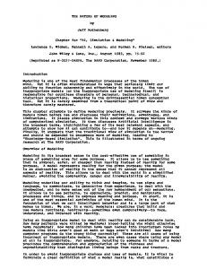
Particle Transport The transport of the nanoscale particles dispersed throughout the fluid is governed by the aerosol GDE. The GDE describes particle dynamics under the influence of various physical and chemical phenomena: convection, diffusion, coagulation, surface growth, nucleation, and the other internal/external forces. The GDE is written in discrete form as a population balance on each cluster or particle size. From a practical point however such a system of equations cannot be solved explicitly except for very small particle sizes - 1000 molecular or “monomer” units. To mitigate this, and other issues, a sectional model to describe the particle size distribution in time and space. The sectional model is advantageous in that there are no a priori assumption regarding
�
i-mers qi-1 q q i i+1
Q
k-1
Sections Q k
Q k+1
Monomers
Size Nucleation/Polymerization Surface growth/Heterogeneous condensation Coagulation/Coalescence
Figure 1: Sectional representation in particle size space. the particle size distribution and does not suffer from the severe constraints of other methodologies.7 The methodology employs a discrete approximation for very small clusters [of molecules] and transition into a sectional representation for the particle size distribution. The sectional model effectively divides the particle size distribution into “bins,” as illustrated in Fig. 1. Instead of solving the GDE, we solve Ns equations, where Ns number of sections. This representation facilitates the capture the physics underlying fluid-particle interactions.
In adopting this framework we can write a general transport equation for the concentration of particles in the kth section, Qk :4
�
∂Qk ∂t
∂Qk u j ∂x j
∂Qk ∂x j
∂ ∂x j
DQ
kb T
Cc 3πµd p
where DQ is the diffusivity is given by
DQ
�
�
ωQ k
�
(4)
(5)
where kb is the Boltzmann constant, Cc is the Cunningham correction factor, and d p is the particle diameter. The source term, ωQ k is given by
�
� � �
�
1 Ns Ns βi j χi jk Qi Q j 2 i∑1 ∑ j 1
ωQ k
�
Ns
�
∑ βik Qi Qk
(6)
i 1
The source term, ωQ k represents the effects of particle-particle interactions: production of Qk due to collisions of smaller particles; the loss and gain of Qk by collision with a particle which either moves the resulting particle out of or into section k; the loss of particles in section k as they collide with each other and form larger particles; and the loss of particles in section k due to collisions with larger clusters. The rate of collision, βi j is given by βi j
�
3 4π
1 6
6kbT ρp
�
1 2
1 vi
�
1 vj
1 2
�
1
vi3
�
�
1
v 3j
�
2
�
(7)
where T is the fluid temperature, vi is the volume of the ith particle, ρ p is the particle density, and χi jk is given by
�� � ���� � � � � � � � ��� νk
χi jk
νi
νk
0
νi
1
νk
1 νj
νk
νj νk νk 1 1
if νk if νk
νi
� 1
otherwise
�
νj
�
νk
� ν�
νi
�
j
1
νk
(8)
The derivation of this form comes from the kinetic theory of gases (the particle diameters are smaller than the mean free path of the carrier gas as is true for gas molecules) under the assumption that inter-particle forces are insignificant (e.g. electrostatic, Van derWaals). Our studies are confined to particles in the free molecule regime Kn 1 This implies that mean free paths over 400nm are expected and growth of aerosols for sizes below this value can be based on one form of the collision frequency function βi j An additional simplification in working at small particle sizes is that the Stokes number is sufficiently small so as to imply that particle velocity slip can be neglected and we can treat the whole problem as a single phase flow, i.e. particle inertial effects can be ignored. Implicit in this formulation of βi j is the assumption that all particles are spherical. This implies that coalescence processes are effectively instantaneous. However, we do know that agglomeration will take place once the collision rate between particles is faster than the coalescence rate, and that this condition is generally reached under combustion conditions growing metal oxides for primary particles greater than about 30nm for most materials (e.g silica, titania, etc.). For our simulations particles are significantly below this threshold value and the assumption of instantaneous coalescence is quite valid. From a more practical standpoint, it has been shown that for small aggregate growth the use of the spherical assumption in the formulation of the collision frequency function underpredicts the collision rate by a factor of two or three. Methods for correction for nonspherical aggregate formation have been developed and provide a convenient and simple modification to the collision frequency function βi j and will included in subsequent work.8
� �
�
Numerical Simulation Procedure The governing transport equations involving the hydrodynamic field are solved using a hybrid MacCormack based compact difference scheme.9, 10 The numerical scheme used is based on the one-parameter family of dissipative two-four schemes (DCPS) developed by Carpenter.10 The accuracy of the scheme is second order in time, and fourth order in space. The DCPS has been shown to be more accurate than other fourth order schemes. All calculations are performed on a rectangular uniformly spaced grid. Though the code has the capacity to solve the equations on a compressed grid, this feature is not used. The exact details of the numerical schemes employed in this study are not given here but a catalog of these schemes, and others, readily available.10, 11
Flow Configuration
���
The configuration consists of a fluid issuing from jet of width D into a co-flowing stream. The space coorx y where x is the streamwise direction, and y is the cross-stream direction. The velocity is dinates are x initialized with a top-hat profile in the cross-stream direction. The initial speeds are Uo and U∞ for the jet and the co-flowing streams, respectively. The velocity ratio is chosen to be Uo U∞ 2 The two streams meet at the inlet plane, x 0 and mix via entrainment and by the motion of the large scale coherent structures.12, 13 While this flow is highly unstable, random perturbations, 3% of Uo in magnitude, are added to the cross-stream velocity in order to accelerate the development of the large scale structures. The jet contains species A which is a passive scalar and can be thought of as a tracer species. As the flow is isothermal T 298K there are no thermophoretic effects, though the incorporation of such effects present no additional difficulty. As the jet travels downstream, particle collisions give rise to new class sizes. A total of ten sections are solved for, ie. Ns 10 This facilitates the solution for particles covering a range of four orders of magnitude in volume. At the jet exit all particles are in the first size class (k 1 d p1 1nm ) thus Qk 0 k 2 3 Ns The volume fraction, or the ratio of the volume occupied by the particles to that occupied by the gas is v f 1 0 10 6 resulting in 1 91 1020 particles exiting the jet each second.
�
�
�
�
�
�
�
� �
�
�
� ����� �
� �
�
�
Numerical Specifications
�
Computations are performed on a domain of 14D by 7D in the streamwise and cross-stream directions, respectively. The computational grid is evenly spaced, ∆x ∆y , and is comprised of 2400 1200 points. With this resolution, a Reynolds number of ReD 4 000 is possible. The molecular Schmidt number is chosen to be Sc 1 The equivalent number for the nanoscale particles, ie the ratio of momentum diffusivity to particle diffusivity, ranges from 2 to 200 Both instantaneous and time averaged data are presented below. This dual view of the hydro-scalar fields allows both qualitative and quantitative assessments. Time averaged data typically employ 50 000 samples, sufficient for two sweeps of the high-speed stream. The sampling process begins tUo after the co-flowing stream has swept through the domain once. At a non-dimensional time of t of 24 (t D ) the values of all variables at every grid point are recorded. The delay in the sampling process allows any initial transients to “wash” through the domain. Sampling continues until t 48 Time-averaged quantities thus correspond to measurements over a period of 2 4 10 4 seconds.
�
�
�
�
�
� �
�
�
�
�
Results
�
Instantaneous contours of the conserved scalar, and the concentration of particles in section 1, Q1 are shown in Fig. 2. This figure illustrates that roughly 90% of the 1nm size particles have coagulated into larger particles
�
�
by x D 4 The conserved scalar, Fig. 2a, portrays the effects of convection and diffusion only; that is, the effects of coagulation are neglected. Under these conditions, the mass of particles in sections 2 through 10 are zero, as they are not present initially and the mechanism which allows particle growth is removed. As the particles collide they grow and thus move from one section, or size class to a larger one. Particles never splinter so there is no movement from larger to smaller sections. The effect of particle coagulation is further illustrated in Fig. 3. This figure shows the instantaneous concentration of particles in section 2, section 3, section 4, section 5, section 9, and section 10; qualitatively it shows that the amount of mass in successive sections peak at further downstream locations. Further, the segregation of particles within vortical structures is observed. Timeaveraged particle concentrations are also considered; centerline particle concentration profiles, Qi along y 0, are shown in Fig. 4a. All concentrations are normalized by the concentration of particles in section 1 at the jet exit. This figure reveals that the peak particle concentration in succeeding sections occurs further downstream. The concentration of particles in section 1 peak at the jet exit, x D 0; section 2 peaks near x D 1 5; section 3 peaks near x D 3; section 4 peaks near x D 6 5; section 5 peaks near x D 9 8; section 6 peaks near x D 11 1; section 7 peaks near x D 13; section 8 peaks near x D 13 5; and the concentration of the remaining sections continue to increase beyond the extent of the computational domain.
� �
�
�
�
�
�
�
�
��
�
�
Because of the two-dimensional flowfield, it is not sufficient to examine the particle field along the centerline. Vortical structures, act to convect particles of all sizes away from the jet center. However, for a sizeable region in space, the hydro-particle dynamics are very similar to what would be observed in a laminar jet, or zerodimensional, flow. The size of this region can be observed by summing the mass of the particle phase along the centerline y 0 The total mass of the particle phase is given by m p T ∑Ni s 1 m p i Qi This quantity (normalized) is shown as a function of downstream distance, x in Fig. 4b. This figure reveals that between x D 0 and x D 9 2 there is no [significant] particle dispersion from the jet center. Thus the particle dynamics in this region should not be different from those in laminar flow, or in a zero-dimensional case between t 0 and t 9 2D Uo Further analysis of the spatio-temporal variation of the particle field is ongoing.
�
�
�
�
�
�
�
� � �
Acknowledgements Support for the first author is provided by the National Science Foundation under Grant ACI-9982274. Computational resources are provided by the Minnesota Supercomputing Institute.
References [1] Dagani, R., NASA Goes Nano, Chem. Eng. News, (1999). [2] Sundaram, S. and Collins, R. L., Collision Statistics in an Isotropic Particle-Laden Turbulent Suspension.Part 1. Direct Numerical Simulations, J. Fluid Mech., 335:75–109 (1996). [3] Walter, C. R. and C., L. R., A Numerical Study of the Particle Size Distribution of an Aerosol Undergoing Turbulent Coagulation, J. Fluid Mech., 415:45–64 (2000). [4] Xiong, Y. and Pratsinis, E. S., Formation of Agglomerate Particles by Coagulation and Sintering Part-I. A 2-D Solution of the Population Balance Equation, J. Aerosol Sci., 24(3):283–300 (1993). [5] Xiong, Y., Akhtar, M., and Pratsinis, E. S., Formation of Agglomerate Particles by Coagulation and Sintering Part II. The Revolution of the Morphology of Aerosol made Titania, silica and Silica-doped Titania Powders, J. Aerosol Sci., 24(3):301–313 (1993).
[6] Pyykonen, J. and Jokiniemi, J., Compuatational Fluid Dynamics Based Sectional Aerosol Modelling Schemes, J. Aerosol Sci., 31(5):531–550 (1999). [7] Zachariah, M. and Semerjian, H., Simulation of Ceramic Particle Formation: Comparison with In-Situ Measurements, AIChE. J., 35:2003 (1989). [8] Matsoukas, T. and Friedlander, S. K., Dynamics of Aerosol Agglomerate Formation, Coll. Int. Sci., (146) (1991). [9] MacCormack, R. W., The Effect of Viscosity in Hypervelocity Impact Catering, AIAA Paper 69-354, 1969. [10] Carpenter, M. H., A High-Order Compact Numerical Algorithm for Supersonic Flows, in Morton, K. W., editor, Twelfth International Conference on Numerical Methods in Fluid Dynamics, Lecture Notes in Physics, Vol. 371, pp. 254–258, Springer-Verlag, New York, NY, 1990. [11] Kennedy, C. A. and Carpenter, M. H., Several new numerical methods for compressible shear-layer simulations, Appl. Num. Math., 14:397–433 (1994). [12] Cain, A. B., Reynolds, W. C., and Ferziger, J. H., A Three-Dimensional Simulation of Transition and Early Turbulence in a Time-Developing Mixing Layer, Department of Mechanical Engineering Report TF-14, Stanford University, Stanford, CA, 1981. [13] Miller, R. S., Madnia, C. K., and Givi, P., Structure of a Turbulent Reacting Mixing Layer, Combust. Sci. and Tech., 99:1–36 (1994).
(a)
(b)
0.0
1.0
�
Figure 2: Instantaneous contours of (a) conserved scalar, Q1 and (b) particle concentration, φ
�
(a)
(b)
(c)
(d)
(e)
(f)
Figure 3: Instantaneous particle concentration contours:(a) section 2, Q2 ; (b) section 3 Q3; (c) section 4 Q4; (d) section 5, Q5; (e) section 9, Q9 ; (f) section 10; Q10.
1.00
1.00 (a)
0.50
0.75 Mtotal
0.75
Qi/Q1
(b)
Q1 Q2 Q3 Q4 Q5 Q6 Q7 Q8 Q9 Q10
0.25
0.00 0.0
0.50
0.25
4.0
8.0 x/D
12.0
16.0
0.00 0.0
4.0
8.0 x/D
12.0
Figure 4: Particle concentration along centerline: (a) Each section; (b) Total concentration.
16.0