Distributed Simulation of Timed Petri Nets - Semantic Scholar

Distributed Simulation of Timed Petri Nets: Exploiting the Net Structure to Obtain ? Eciency Giovanni Chiola1 and Alois Ferscha2 Universita di Torino, Dipartimento di Informatica I-10149 Torino, Italy Universitat Wien, Institut fur Statistik und Informatik A-1080 Vienna, Austria 1

2

Abstract. The conservative and the optimistic approaches of distributed discrete event simulation (DDES) are used as the starting point to develop an optimized simulation framework for studying the behaviour of large and complex timed transition Petri net (TTPN) models. This work systematically investigates the interdependencies among the DDES strategy (conservative, Time Warp) and the spatial decomposition of TTPNs into logical processes to be run concurrently on individual processing nodes in a message passing and shared memory multiprocessor environment. Partitioning heuristics are developed taking into account the structural properties of the TTPN model, and the simulation strategy is tuned accordingly in order to attain the maximum computational speedup. Implementations of the simulation framework have been undertaken for the Intel iPSC/860 hypercube, the Sequent Balance and a Transputer based multiprocessor. The simulation results show that the use of the Petri net formalism allows an automatic extraction of the parallelism and causality relations inherent to the model.

1 Introduction The popularity of the timed Petri net modelling and analysis framework for the quantitative (and simultaneously qualitative) study of asynchronous concurrent systems is mainly due to the availability of software packages automating the analysis algorithms and often providing a powerful, graphic user interface. Although the use of Petri net tools shows that complex simulation models are hard and costly to evaluate, simulation is often the only practical analysis means. Parallel and distributed simulation techniques have in some practical applications, and at least in theory, improved the performance of large systems simulation, but are still far from a general acceptance in science and engineering. The main reasons for this pessimism are the lack of automated tools and simulation languages ?

The work at the University of Torino was performed in the framework of the Esprit BRA Project No.7269, QMIPS. The work at the University of Vienna was nancially supported by the Austrian Ministry for Science and Research under Grant GZ 613.525/2-26/90.

suited to parallel and distributed simulation, as well as performance limitations inherent to the simulation strategies. This paper points out the special suitability of the Petri net formalism for parallel and distributed simulation: it allows an automatic exploitation of useful model parallelism by structural Petri net analysis; moreover, based on some Petri net properties, simulation strategy can be designed in order to optimize overall execution time. Causal relations among events are explicitly described by the Petri net structure so that a proper exploitation of this information may potentially improve the performance of general purpose, distributed simulation engines. A TTPN is decomposed into a set of spatial regions that bear potentially concurrent events, based on a preanalysis of the net topology and initial marking. The decomposed TTPN is assigned to multiple processors with distributed memory, working asynchronously in parallel to perform the global simulation task. Every processor hence simulates events according to a local (virtual) time and synchronizes with other processors by rollbacks of its local time caused by messages with time stamp in the local past | thus no synchronous communication is required at the software level (neither the send nor the receive message operations are blocking to the processors). Input buers are assumed to be available for every processor to keep arriving messages until they are withdrawn by an input process between the simulation of two consecutive events.

1.1 Timed Transition Petri Nets In the sequel of this work we consider the class of timed Petri net models where timing information is associated to transitions [1]:

De nition 1.1 A timed Petri net is a tuple TTPN = (P; T; F; W; ; ; M ) where:

0

(i) P = fp1; p2; : : :; pnP g is a nite set of P -elements (places), T = ft1 ; t2; : : :; tnT g is a nite set of T -elements (transitions) with P \ T = ; and a nonempty set of nodes (P [ T 6= ;). (ii) F  (P  T) [ (T  P) is a nite set of arcs between P -elements and T elements denoting input ows (P  T ) to and output ows (T  P ) from transitions.

(iii) W : F 7! IN assigns weights w(f) to elements of f 2 F denoting the multiplicity of unary arcs between the connected nodes.

(iv)  : T 7! IN assigns priorities i to T -elements ti 2 T . (v)  : T 7! IR assigns ring delays i to T -elements ti 2 T . (vi) M0 : P 7! IN is the marking mi = m(pi ) of P -elements pi 2 P with tokens in the initial state of TTPN (initial marking). A transition ti with i = (ti ) is said to be enabled with degree k > 0 at priority level i in the marking M, i k > 0 is the maximum integer such that 8pj 2  ti , m(pj )  k w(pj ; ti) in M (  ti = fpj j (pj ; ti ) 2 F g and ti = fpj j (ti ; pj ) 2 F g). ti is said to be enabled with degree k > 0, i there

are no transitions enabled with positive degree on a priority level higher than i. The multiset of all transitions enabled in M (with positive enabling degree representing the multiplicity of the transition) is denoted E(M). A transition instance ti that has been continuously enabled during the time i must re, in that it removes w(pj ; ti ) tokens from every pj 2  ti by at the same time placing w(ti; pk ) tokens into every pk 2 ti . This ring of a transition takes zero time and is denoted by M[tiiM 0.

1.2 Approaches to DDES in the Literature Discrete event simulations of TTPNs exploit a natural correspondence between transition rings and event occurrences: an event in the simulated system relates to the ring of a transition in the TTPN model. In general, a simulation engine (SE) maintains an ordered list of time stamped events (transitions) scheduled for their occurrence ( ring) time and repeatedly executes the rst event in the list by simulating the behaviour caused by the event. The virtual time of the simulation is changed to the event's timestamp; new events caused are scheduled and events having lost their cause are descheduled. In terms of the TTPN model the marking is changed according to the transition ring, and newly enabled (disabled) transitions are scheduled (descheduled). Distributed simulation strategies generally aim at dividing a global simulation task into a set of communicating logical processes (LPs) trying and exploiting the parallelism inherent in the concurrent execution of these processes. With respect to the target architecture we distinguish among parallel discrete event simulation if the implementation is for a tightly coupled multiprocessor allowing simultaneous access to shared data (shared memory machines), and distributed discrete event simulation (DDES) if loosely coupled multiprocessors with communication based on message passing are addressed. In this work we only restrict to DDES. Notice however that the simulation algorithms developed for DDES trivially adapt to the execution on shared memory multiprocessors without performance loss. Indeed event processing must respect causality constraints even in parallel and distributed simulation:classical DDES approaches preserve causality by simply enforcing timestamp ordering in event processing. Two main protocols have been proposed for the implementation of DDES: conservative that enforces time stamp order processing by restricting the parallelism among LPs and optimistic that instead allows out of timestamp order to occur and then correct the situation by \undoing" part of the simulation. Both, the conservative [2] and the optimistic strategy [3] have led to implementations of general purpose discrete event simulators on parallel and distributed computing facilities (for a survey see [4]). The main potential contribution of the use of Petri net model descriptions for DDES is to de ne causality relations explicitly through the graph structure, thus allowing one to relax constraints on timestamp ordering for the processing of events that are not causally related. From this consideration we can thus expect to be able to increase the parallelism of a DDES engine with respect to the

standard approaches by just taking the structure of the PN model into proper account. In conservative DDES strategies all interactions among LPs are based on timestamped event messages sent between the corresponding LPs. Out-of-timeorder processing of events in LPs is prevented by forcing LPs to block as long as there is the possibility for receiving messages with lower timestamp, which in turn has a severe impact on simulation speed. Optimistic DDES strategies weaken this strict synchronization rule by allowing a preliminary causality violation, which is corrected by a (costly) detection and recovery mechanism usually called rollback (in simulated virtual time). In order to guarantee a proper synchronization among LPs in optimistic simulation, two rollback mechanisms have been studied. In the original Time Warp [3] an LP receiving a message with timestamp smaller than the LPs locally simulated time (straggler message) starts a rollback procedure right away. Rollback is initiated by revoking all eects of messages that have been processed prematurely by restoring to the nearest safe state, and by neutralizing, i.e. sending \antimessages" for messages sent since that state (aggressive cancellation, ac). The impact of the erroneously sent messages is that also succeeding LPs might be forced to rollback, thus generating a rollback chain that eventually terminates. Reducing the size of the rollback chain is attempted by \ ltering" messages with preempted eects, by postponing erroneous message annihilation until it turns out that they are not reproduced in the repeated simulation (lazy cancellation, lc) [5], or by maintaining a causality record for each event to support direct cancellation of messages that will de nitely not be reproduced. The performance of rollback mechanisms is investigated in [6] and [7].

1.3 Paper Organization

The balance of the rest of this paper is the following. Section 2 introduces classical concepts of DDES and adapts them to the particular case of TTPN models. Dierent kinds of customizations of DDES strategies and partitioning in concurrent LPs are discussed in a general framework. Section 3 presents empirical results derived from the implementation of several variations of DDES strategies for TTPN models on 3 dierent multiprocessor architectures. Results are analyzed to identify weaknesses and potentialities of the dierent alternatives and to validate some of the proposed net speci c optimizations. Section 4 outlines additional optimizations that may be introduced in the most promising DDES strategy to take into account particularly favourable net topologies. Section 5 contains concluding remarks and perspectives for future developments of the research.

2 A Distributed Simulation Framework for TTPNs 2.1 Logical Processes

In the most general case of distributed simulation of TTPNs we consider a decomposition of the \sequential" discrete event simulation task into a set of

communicating LPs to be assigned to individual processing elements working autonomously and communicating with each other for synchronization. Each and only one LP is assigned to a dedicated processor and is residing there for the whole real simulation time. A message transportation system is assumed to be available (either implemented fully in software or by hardware routing facilities) that implements directed, reliable, FIFO communication channels among LPs. Every LP applies one and the same discrete event strategy to the simulation of the local subnet. We identify the work partition assigned to LPs, the LPs' communication behaviour and the LPs' simulation strategy as the constituent parts of a distributed simulation framework, and will in further treat these three components in a very abstract form. De nition 2.1 A Logical Process is a tuple LPk = (TTPNRk; Ik ; SE) where (i) region TTPNRk = (Pk ; Tk ; Fk  (Pk  Tk ) [ (Tk S Pk ); W; ; ; M 0) is a (spaSN N LP LP T , F = tial) region of some TTPN such that P = k=1 Pk , T = k=1 k SN LP F S ((P  T ) [ (T  P )) , which are again k i k i k k=1 i2neighborhood(TTPNRk ) TTPNs in the sense of De nition 1.1,

(ii) communication interface Ik = (CH; m), theScommunicationinterface of LPk is a set of communication channels CH = k;i chk;i where chk;i = (LPk ; LPi) is a directed channel from LPk to LPi , corresponding to an arc f 2 F and carrying messages m = hw(f); D; TT i where w(f) (wf for short) is the number of tokens transferred, D is an identi er of the destination (place or transition) and TT (token time) is the timestamp of the local virtual time of the sending LPk at send time. (iii) simulation engine SE is a simulation engine implementing the simulation strategy. S The set S of all LPs LPS= k LPk together with directed communication channels CH = k;i chk;i = k;i(LPk ; LPi) constitute the Graph of Logical Processes GLP = (LP; CH). Within the frame of this general de nition of a logical simulation process a variety of dierent distributed simulations are possible. Not all combinations of decompositions into regions, communication interfaces and simulation engines make sense in practical situations: most of the combinations will not conform to the expectations of increasing simulation speed over sequential simulation. Moreover they are highly interrelated: e.g. the simulation engine aects the communication interface and the appropriateness of decompositions. To the best of our knowledge three approaches have been developed so far in the literature ([8], [9], [10]), which would be categorized according to our framework as follows. In [8] an LP is created for every p 2 P and every t 2 T, resulting in a very large number of LPs (j LP j=j P j + j T j) of smallest possible grain size, where the maximum number of arcs between any pair of LPs is 1. The idea behind this partition choice is to maximize the \potential parallelism" of

the DDES in terms of number of LPs. For every arc an unidirectional channel with the same orientation as the arc is introduced. For every input arc from a place's LP and a transition's LP another unidirectional channels with the opposite orientation is required (control channel) in order to solve con icts. The Ik proposed is based on a protocol invoking four messages (\activate," \request," \grant," and \con rm") among a transition's LP and all its input places' LPs in order to re the transition. Obviously the (possibly tremendous) amount of messages inherent to this approach prevents eciency if simulated in a distributed memory environment (their protocol has been simulated on a shared memory multiprocessor). The proposed simulation engine is conservative. Another conservative approach has been introduced by [9], allowing \completely general" decompositions into regions and employing a simulation engine that handles three kinds of events: the arrival of a token, the start and the end of transition ring in order to exploit lookahead. The generality of the partition is limited in such a way that con icting transitions together with all their input places are always put together in the same LP, in order to avoid distributed con ict resolution. Recently [10] a Time Warp simulation (i.e., a simulation engine following the optimistic approach) of SPNs has been proposed also allowing any partitioning in the TTPNRk sense, but with a redundant representation of places (and the corresponding arcs) in adjacent LPs. Their Ik maintains time consistency of markings among LPs by exchanging ve dierent types of messages. The freedom of allowing any partitioning that stems from arbitrary arc cutting makes the message exchange protocol and the simulation engine unnecessarily complex. In the following we systematically work out useful, (and then improved) combinations of TTPN regions, communication interfaces and simulation engines.

2.2 TTPN Regions

The most natural decomposition of work is the spatial partitioning of a TTPN into disjoint regions TTPNRk representing small(er) sized TTPNs. This also supports the application of one and the same simulation engine to all regions. Apparently the decomposition of a TTPN has strong impact on the DDES performance. Small sized regions naturally raise high communication demands, whereas large scale regions can help to clamp local TTPN behaviour inside one LP. The common drawback of the intuitive partitionings in [8] and [10] is the necessity of developing a proper communication protocol among LPs in order to implement a distributed con ict resolution policy for transitions sharing input places. In a message passing environment for inter process communication, such a con ict resolution protocol may induce substantial overhead in the distributed simulation, thus nullifying the advantages of the potential model parallelism on the simulation time. \Arbitrary arc cutting" for partitioning can burden performance since arcs f 2 (P  T) have a (severe) consequence on the ecient computation of enabling and ring, whereas arcs out of (T  P) have not such consequence. The latter is the reason why the partitioning has to be related to the TTPN ring rule: an LP is a minimum set of transitions Tk along with

S

its input set (  (Tk ) = ijti 2Tk  ti ) such that local information is sucient to decide upon the enabling and ring of any ti 2 Tk . This is in order to minimize con ict resolution overhead, since in this way con ict resolution always occurs internally to an LP, thus involving no communication overhead.

Minimum Regions Let CS(ti ) be the set of all transitions tj 2 T in structural con ict with ti (ti ; tj 2 T are said to be in structural con ict denoted by (ti SC tj ), i  ti [  tj = 6 ;. In the case of GSPNs with priority structures [11] extended con ict set ECS(ti ) have been de ned as the sets of all transitions tj 2 T in indirect structural con ict with ti . To relate the region partitioning to the ring semantics de nition of TTPNs, all transitions within the same CS (or ECS) have to be included in the same TTPNRk , since a distribution over several regions would require distributed con ict resolution (which would in any case degrade performance). This consideration leads directly to a partitioning into minimum regions, i.e. TTPNRk s that should not be subdivided further in order to be practically useful: LP T De nition 2.2 TTPNRk = (Pk ; Tk ; Fk ; W; ; ; M0) of some TTPN, SNk=1 k = T , where Tk = fti g, ti 2 T is a single transition i ti 2 T does not participate in any ECS or Tk = S ECS(ti )  T , ti 2 T is the whole ECS i ti 2 T participates in some ECS, Pk = ti 2Tk  (ti ) and Fk  (Pk  Tk ) is called a minimum region of TTPN.

Any general TTPN can always (and uniquely) be partitioned into minimum regions according to De nition 2.2.

2.3 The Communication Interface

Of course, the decomposition of TTPNs requires an interface among TTPNRs preserving the behavioural semantics of the whole TTPN. Such an interface has to be implemented by an appropriate communication protocol among the regions, according to the strategy chosen for the simulation engines. Since we have forced the regions not to distribute p 2 Pi and t 2 Tk over dierent regions TTPNRi and TTPNRk if there exists an arc f = (p; t) 2 (Pi  Tk ) (remember that for each TTPNRk, ti 2 Tk )  (ti ) 2 Pk ), we can map the sets of arcs (Tk  Pj )  F interconnecting dierent TTPN regions to the channels of the communication interface. In other words we de ne Ik = (CH; m) of TTPNRk to be the communication interface with channels CH = S k;i chk;i, where chk;i = (LPk ; LPi ) is a set of directed channel from LPk to LPi , corresponding to all the arcs (tl ; pm ) 2 (Tk  Pi)  F, tl 2 Tk , pm 2 Pi, carrying messages m of identical type. A message m represents tokens to be deposited in places of adjacent LPs due to the ring of local transitions. The description (and implementation) of the interaction among LPs is also simpli ed in theSfollowingway. Consider two TTPN regions TTPNRi and TTPNRj , inand let Ti.j = l tl j (tl ; p) 2 (Ti  Pj ) be the set of transitions in TTPNR Si cident to arcs pointing to places in TTPNRj , and analogously Pj/i = l pl j

(t; pl ) 2 (Ti  Pj ) the set of places in TTPNRj incident to arcs originating from transitions in TTPNRj , then the interaction of LPi and LPj only concerns Ti.j and Pj/i. We call Ti.j (Pj/i) the output border (input border) of TTPNRi towards S . TTPNRj (of TTPNR j from TTPNRi). Tk = i Tk.i is the output border of S /i / TTPNRk , Pk = i Pk is the input border. (Naturally, Pk/ = Pk and Tk. = Tk for a minimum region.) As a static measure of the potential communication induced by LPi we can de ne its arc-degree (of connectivity ) as the number of arcs f 2 F originating in TTPNRi and pointing to places in adjacent TTPNRs and vice-versa: AD(TTPNRi) =



[

(Pi  Tk ) [ (Tk  Pi)

k2neighborhood(TTPNRi )



Similarly we de ne the channel-degree CD(TTPNRi) =

[

k

chi;k j + j

[

k

chk;i



as the number of channels connected to a region. Note that these measures can be evaluated in a static preanalysis of the decomposed TTPN.

LPi Input Border

Output Border

Input Border LPj

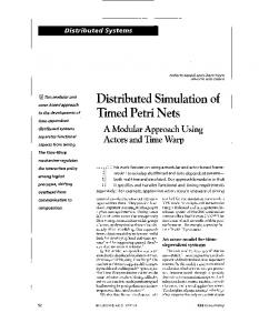
Fig. 1. TTPN Region for a Logical Process. Figure 1 shows a TTPN region to become the \local simulation task" of some LP. The set of dashed TTPN arcs from LPi to LPj represent the directed communication channel among them. The arc-degree of connectivity of LPi in Fig. 1 is 7, while a single channel is needed to connect LPi to LPj , thus inducing a channel-degree  5 for LPi . Figure 2 shows the minimum region partitioning | De nition 2.2 | of a GSPN model of the reader-writer problem [11].

N=3 reading endR

isread Rqueue choice

think

N

arrival

LP1

startR

notacc

N

_N

LP3 startW

LP2

LP4

iswrite Wqueue

LP5 endW

writing

_N

Fig.2. Reader/Writer Example: Minimum Region Partitioning.

2.4 The Simulation Engine A general simulation engine (SE) implements the simulation of the occurrence of events in virtual time according to their causality; at the same time it collects a trace of event occurrences over the whole simulation period. Data structures of a general SE include: the TTPN representation (in some internal form); an event list (EVL) with entries ek = hti @FT i ( re transition ti at time FT); the virtual time (VT); the event stack (ES) with entries of the form hti ; V T; M i (ti is the transition that has red at virtual time VT, yielding a new marking M). An optimized discrete event SE [12] [13] exploits structural properties of the underlying TTPN in order to speed up simulation time: Let ti ; tj 2 T be causally connected denoted by (ti CC tj ) (i.e. given ti 2 E(M) and tj 62 E(M), then M[ti iM 0 might cause that tj 2 E(M 0 )) and CC(ti ) the set of all transitions causally connected to ti, then the ring of ti has a potential enabling eect only on transitions in SPE(ti ) = CC(ti). Call SPE(ti ) the set of potential enablings of ti . Analogously a set of potential disablings SPD(ti ) can be de ned: Let ti; tj 2 T be mutually exclusive (denoted by (ti ME tj )), i.e. they cannot be simultaneously enabled in any reachable marking, and ME(ti ) the set of all transitions mutually exclusive to ti , then the ring of ti has a potential disabling eect only on transitions in SPD(ti ) = SC(ti ) ? ME(ti ) (SC(ti ) is the set of transitions in structural con ict to ti ). The gain of this TTPN structure exploitation is that after every transition ring only SPE(t) and SPD(t) have to be investigated rather than the whole T, which is signi cant for j SPE(ti ) j, j SPD(ti ) j j T j. The (optimized) SE behaves as follows. After an initialization and a preliminary scheduling of events caused by the initial marking the algorithm performs | if there are events to be simulated | the following steps until some end time is reached. First all simultaneously enabled transitions are generated and con ict is resolved identifying one transition per actual con ict set to be red; the rst scheduled transition is red in that it is removed from EVL, the marking is changed accordingly, possible new (obsolete) transition instances are sched-

uled (descheduled) by insertion (deletion) of new (old) events into (from) EVL (investigating only SPE and SPD !); the occurrence of the event at its virtual simulated time and the new marking are logged into ES, and the VT is updated to the occurrence time of the event processed. This (sequential) general SE is adapted to DDES strategies as described in the following sections.

2.5 The Conservative Strategy The SE following the conservative approach allows only the processing of safe events, i.e. the ring of transitions up to a local virtual time LVT for which the LP has been guaranteed not to receive token messages with timestamp \in the past." The causality of events is preserved over all LPs by sending timestamped token messages of type m = hw; D; TT i (with w > 0) in non decreasing order, or at least a promise m = h0; D; TT i (null message ) not to send a new message time-stamped earlier than TT, and by processing the corresponding events in nondecreasing time stamp order. One basic practical problem is the determination of when it is safe to process an event, since the degree to which LPs can look ahead and predict future events plays a critical role in the performance of the DDES. For conservative DDES so called \lookahead" coming directly from the TTPN structure can be exploited. Given some transition ti located in the output border of some LPk (ti 2 Tk. ). ti is said to be persistent if there is no tj 2 Tk such that if ti ; tj 2 E(M), and M[tj iM 0 causes that ti 62 E(M 0) for all reachable markings M. A sucient condition for persistence of ti is that 8tj ;  ti \  tj = ;. Call tj the persistent predecessor of ti if  ti = tj and 8k 6= j;  ti \ tk = ;; let Tkpers (ti ) be the set of all persistent predecessors ahead of ti, i.e. the transitive closure of the persistent predecessor relation. Then a lower bound for the degree of lookahead exposed P by LPk via ti is j jtj 2Tkpers (ti ) j , i.e., the sum over all ring times of transitions in Tkpers (ti ).

De nition 2.3 Let ti 2 Tk. and tj 2 Tk be persistent ((  ti) = ti ; (  tj ) = tj ). ti and tj are said to be in the same persistence chain denoted by the set (tj ; ti ), i there exists a sequence S = ftr ; ts : : :ttg of persistent predecessors (tr ; ts : : :tt 2 Tk ) such that tj 2 E(M) ) ti 2 E(M 0) M[S iM 0 . Since every t 2 S is persistent, we can state the following: Corollary 2.1 Given that tj 2 Tk ;i2 Tk. and PM with tj 2 E(M) at time  , then M 0 with ti 2 E(M 0) is reached at time  + t2S (t) at the earliest. For two transitions tj 2 Tk ; ti 2 Tk. in the same persistencePchain we can de ne the amount of lookahead of tj on ti by la((tj ; ti )) = t2 tj ;ti (t) (with the particular case la((tj ; ti )) = 0 if (tj ; ti ) = ;). The value of la can (

)

be established for all pairs of transitions in the TTPN region (one in the output border, the other not in the output border) by a static preanalysis of the region structure. This can improve the simulation performance since upon ring of

any transition within some TTPNRk the timestamp of output messages caused by transitions in the output border which are in the same persistence chain can be increased (and thus improved) by la, thus relaxing the synchronization constraints on the adjacent LPs. Assuming that the communication requirements of GLP = (LP; CH) are supported by the multiprocessor hardware (i.e. there exist communication media for all chk;i = (LPk ; LPi)), then we derive the following conservative simulation engine SE co to be applied in every LPi 2 LP. Two types of messages are necessary to implement the communication interface: token messages m = hwf ; D; TT i carrying a speci c number of tokens (wf or #) to some destination place D (which uniquely de nes the destination LP), and null messages m = h0; D; TT i. SE co holds the net data of TTPNRk and simulates the local behaviour of the region by holding transitions to be red in a local EVL, recording event occurrences in a local ES and incrementing a local time LVT. For every input channel an input queue collects incoming messages, the rst element of which (that de nes the channel clock, CC) is used for synchronization. Output buers OB keep messages to be sent to other LPs, one per output channel. The behaviour of SE co is to process the rst event of EVL if there is no token message in one of the CCi s with smaller timestamp (process rst event ), or to process the token message with the minimum token time (process rst message ). Processing the rst event (i.e., ring transition t) is similar to the general SE (change marking, schedule/deschedule events, increment LVT), but also invokes the sending of messages: If t 2 Tk. then a message h#; D; LV T i is generated and deposited in the corresponding OB; if t 62 Tk. then a null message h0; D; LV T +la((t ; ti )) is deposited for every ti 2 Tk. in the corresponding OBs { thus giving maximum lookahead to all the following LPs. After processing the rst event the contents of all OBs is transmitted, except for null messages with token times that have already been distributed in a previous step (to reduce the number of null messages). The processing of the rst message invokes removing the message with minimum timestamp over all CCi s from CCi (the head of IQi ), while leaving a \null message copy" (change # to 0 in the message head) of it in CCi if it has been the last message in IQi . M and LVT are changed accordingly; also scheduling/descheduling of events might become necessary.

2.6 Time Warp Strategies

In order to simulate a TTPNRk according to the Time Warp (optimistic) strategy [14] one input queue IQ and one output queue OQ with time sequenced message entries are maintained. Either positive (token) messages (m = hwf ; D; TT; `+'i) or negative (annihilation) messages (m = hwf ; D; TT; `?'i) are received from other LPs out of GLP = (LP; CH) not necessarily in time stamp order, indicating either the transfer of tokens or the request to annihilate a previously received positive message. Messages are assumed to be buered in some input buer IB upon their arrival, to be taken over into IQ eventually. Messages generated during a simulation step are held in an output buer OB to be sent upon completion of the step itself, all at once. The data structure of an LP with

an optimistic SE (SE opt ) is depicted in Fig. 3; a simulation engine is shown in Fig. 4. SE opt behaves as follows: rst all ti 2 Tk enabled in M0 are scheduled. Messages received are processed according to their timestamp and sign; messages with timestamp in the local future (tokentime (m) > LVT) are inserted into IQ (if the sign of m is `+' then it is inserted in timestamp order, a message with sign(m) = `?' annihilates its positive counterpart in IQ. Straggler messages (tokentime (m) < LVT) force the LP to roll back in local simulated time by restoring the most recent valid state. Processing the rst event (as in SEco ) simulates the ring of a transition and the generation of output messages, while processing the rst message changes M and possibly schedules/deschedules new/old events. Whenever an event is processed the event stack ES additionally records all state variables such that a past state can be reconstructed on occasion. The algorithm requires the knowledge of the global virtual time (GVT), a lower bound for the timestamp of any unprocessed message in GLP = (LP; CH), in order to reduce bookkeeping eorts for past states (ES).

LVT EVL < tk@ Input Channels IB # P

# P

# P

-

+

+

GVT > < ti@

> < tj@

IIIIIIIII IIIIIIIII IQ IIIIIIIII IIIIIIIII + + + + + + IIIIIIIII IIIIIIIII IIIIIIIII OQ IIIIIIIII IIIIIIIII + + + + + + IIIIIIIII GVT # P

# P

# P

# P

# P

# Pi

GVT # P

# P

# P

# P

# P

# Px

ES

# Pj

# Pk

+

+













>

... Output Channels OB # Px

+

IIIIIIIIIII IIIIIIIIIII IIIIIIIIIII IIIIIIIIIII IIIIIIIIIII IIIIIIIIIII

Fig. 3. Logical Process for Optimistic Strategies Rollback can be applied in two dierent ways. An optimistic simulation engine with aggressive cancellation (SEac , see Fig. 5) rst inserts the straggler message into IQ, and sets LVT to tokentime(m). Then the state at time LVT is restored, which is the marking at time of the already processed event closest but not exceeding LVT in SQ. All messages in OQ with token time larger than the rolled back LVT are annihilated by removing them from OQ and sending corresponding antimessages. Finally, all records prematurely pushed in the

program SEopt (TTPNk ) S1 GVT:=0; LVT := 0; EVL := fg; M := M ; stop := false; S2 for all ti 2 E(M ) do schedule(hti @i i) od S3 while not stop do S3.1 for all m 2 IB do S3.1.1 if tokentime(m) < LV T S3.1.1.1 then rollback(tokentime(m), m) else insert(IQ, m) od S3.2 if EVL = fg ^ IQ = fg then goto S3.1 S3.3 if (GVT  endtime) ^ (not empty(EVL)) do S3.3.1 if tokentime( rst(EVL)) < tokentime( rst(IQ)) S3.3.1.1 then process( rst(EVL)) else process( rst(IQ)) od S3.4 for all m 2 OB do send(m) od S3.5 if (GVT  endtime) then stop := true; S3.6 od while 0

0

Fig. 4. Aggressive Cancellation Simulation Engine for TTPNk . procedure rollback(time, m) S1 S2 S3 S4 S4.1 S4.2 S5

/* aggressive cancellation */ LVT := time insert(IQ, m) restore-state(LVT) for all m 2 OQ with tokentime(m)  LV T do insert(OB, htokencount(m); outplace(m); tokentime(m); `?' i); delete(OQ, m) od pop(ES, LVT)

Fig. 5. Aggressive Cancellation Rollback Mechanism. STST are popped out (line S5). A lazy cancellation optimistic simulation engine (SElc ) would keep the negative messages generated in an intermediate list (S4.1: insert(IL, htokencount(m); outplace(m); tokentime(m); `?'i)), and move that (negative) m to OB only in the case that resimulation has increased LVT over tokentime(m). In the case that reevaluation yields exactly the same positive message as already sent before, the new positive message is not resent, but used to compensate the corresponding negative message from IL | thus annihilating the (obsolete) causality correction locally, and preventing from unnecessary message transfers as well as possibly new rollbacks in other LPs.

3 Performance In uences Due to the variety of degrees of freedom in composing a DDES for TTPNs as oered by the framework developed above, the question for optimizing the performance of a distributed simulation on a physical multiprocessor naturally

arises. We have implemented the SEs and communication interfaces for a 30 node Sequent Balance, a 16 node Intel iPSC/860 and a 16 node T800 Transputer multiprocessor. Case studies showed that there are in uences on the performance of the distributed simulation which are inherent to a proper combination of the partitioning in regions (TTPNRk s), the communication interface (Ik s) and the simulation engine, but also caused by the physical hardware as such. In the following we will evaluate the main observations and use the empirical results for an improved distributed simulator for TTPNs. We consider the small net depicted in Fig. 2 as a test case since the automatic partitioning of arbitrary nets is still under development and for the time being the partitioning has to be hand coded in our prototypes. In practice one would apply DDES techniques to substantially larger models. However the test case is signi cant since it exhibits most of the characteristic features of larger models and the results may be extrapolated for larger nets.

3.1 Partitioning We already proposed a partitioning such that several transitions together with all their input places are simulated by a single logical process. Subnets are constructed from the topologic description of the TTPN so that con ict resolution always occurs internally to a logical process. Depending on the particular multiprocessor architecture on which the DDES is run, such minimal region partitioning may however turn out to be too ne grain to eciently adapt to the interprocessor communication overhead. One should thus be willing to partition the DDES in a lower number of LPs in order to reduce the communication overhead and attain better performance. In practice a trade-o must be sought for dierent target architectures based on empirical cases in order to achieve speedup over sequential simulation. Figure 6 compares (in the 5 LP columns) absolute execution time of the minimum region partitioning with a SElc of the reader writer net in Fig. 2 in a balanced parametrization: arrival = 1:0, endR = 2:0, endW = 0:5, prob(isread) := 0:8, prob(iswrite) := 0:2 and N = 4 processes. The results show that the Sequent Balance takes physically more communication time, although the work pro le is the same as for the iPSC, which uses a faster processor. From the communication overheads encountered for the minimumregion partitioning it is obvious to see that the communication/computation ratio has to be increased to use this kind of multiprocessor hardware more eciently. Moreover, additional aggregation of con ict sets into larger logical simulation processes may increase the balancing of the distributed simulation without decreasing its inherent parallelism if some conditions are veri ed on the TTPN model structure (grain packing). For example transitions endR and endW are never simultaneously enabled, thus LP4 and LP5 in Fig. 2 can be aggregated to a single LP without loss of potential model parallelism. The following rules can be applied to pack grains starting from minimum TTPNRk s:

Sequent Balance B21 160

Intel iPSC/860

5 LP5

5 LP4

5 LP3

5 LP2

AAAAAAAA AAAAAAAA AAAA AAAAAAAA AAAAAAAA AAAA AAAAAAAA AAAAAAAA AAAA AAAA AAAA AAAA AAAA AAAA AAAA AAAA AAAA AAAA AAAA AAAAAAAA AAAA AAAA AAAA AAAAAAAA AAAA AAAA AAAA AAAAAAAA AAAA AAAA AAAA AAAAAAAA AAAA AAAA AAAA AAAAAAAA AAAA AAAA AAAA AAAAAAAA AAAA AAAA AAAA AAAAAAAA AAAA AAAA AAAA AAAAAAAA AAAA AAAA AAAA AAAAAAAA AAAA AAAA AAAA AAAA AAAA AAAA AAAA AAAA AAAA AAAA AAAA 5 LP1

3 LP3

3 LP2

AAAA AAAA AAAA AAAA AAAA AAAA AAAA AAAA AAAA AAAA AAAA AAAA AAAA AAAA AAAA AAAA AAAA AAAA AAAA AAAA AAAA AAAA AAAA AAAA AAAA AAAA AAAA AAAA AAAA AAAA AAAA AAAA AAAA AAAA AAAA 3 LP1

AAAA AAAA AAAA AAAA AAAA AAAA AAAA AAAA AAAA AAAA AAAA AAAA AAAA AAAA AAAA AAAA AAAA 2 LP2

3 LP3

3 LP2

2 LP2

2 LP1

0

event processing

2 LP1

20

AAAA AAAA termination protocol AAAA AAAA AAAA blocking AAAA AAAA AAAA rollback AAAA communication AAAA

1 LP1

40

5 LP5

60

5 LP4

80

5 LP3

100

5 LP2

3 LP1

120

AAAA AAAA AAAAAAAA AAAA AAAA AAAA AAAA AAAA AAAA AAAAAAAA AAAA AAAA AAAAAAAA AAAA AAAAAAAA AAAA AAAA AAAA AAAA AAAA AAAA AAAAAAAA AAAA AAAA AAAA AAAAAAAA AAAA AAAA AAAA AAAAAAAA AAAA AAAA AAAA AAAAAAAA AAAA AAAA AAAA AAAA AAAA AAAA AAAA AAAA AAAAAAAA AAAA AAAA AAAA AAAA AAAA AAAA AAAA AAAA AAAAAAAA AAAA AAAA AAAA AAAA AAAAAAAA AAAA AAAA AAAAAAAA AAAA AAAA AAAA AAAAAAAA AAAA AAAA AAAA AAAAAAAA AAAA AAAA AAAA AAAAAAAA AAAA AAAA AAAA AAAAAAAA AAAA AAAA AAAA AAAAAAAA AAAA AAAA AAAA AAAAAAAA AAAA AAAA AAAA AAAAAAAA AAAA AAAA AAAA AAAAAAAA AAAA AAAA AAAA AAAAAAAA AAAA AAAA AAAA AAAAAAAA AAAA AAAA AAAA AAAAAAAA AAAA AAAA AAAA AAAAAAAA AAAA AAAA AAAA AAAAAAAA AAAA AAAA AAAA AAAAAAAA AAAA AAAAAAAA AAAA AAAA AAAA AAAA AAAA AAAAAAAA AAAA AAAA AAAA AAAAAAAA AAAA AAAA AAAA AAAAAAAA AAAA AAAA AAAA AAAAAAAA AAAA AAAA AAAA AAAAAAAA AAAA AAAA AAAA AAAAAAAA AAAA AAAA AAAA AAAAAAAA AAAA AAAA AAAA AAAAAAAA AAAA AAAA AAAA AAAAAAAA AAAA AAAA AAAA AAAAAAAA AAAA AAAA AAAA AAAA AAAAAAAA AAAA AAAA AAAAAAAA AAAA AAAA AAAA AAAA AAAA AAAA 5 LP1

AAAA AAAA AAAA AAAA AAAA AAAA AAAA AAAA AAAA AAAA AAAA AAAA AAAA AAAA AAAA AAAA AAAA AAAA AAAA AAAA AAAA AAAA AAAA AAAA AAAA AAAA AAAA AAAA AAAA AAAA AAAA

AAAA AAAAAAAA AAAA AAAAAAAA AAAA AAAAAAAA AAAA AAAA AAAA AAAA AAAA AAAA AAAA AAAA AAAA AAAA AAAA AAAA AAAA AAAA AAAA AAAAAAAA AAAA AAAA AAAA AAAA AAAA AAAA AAAA AAAA AAAA AAAAAAAA AAAA AAAA AAAAAAAA AAAA AAAAAAAA AAAA AAAAAAAA AAAA AAAAAAAA AAAA AAAAAAAA AAAA AAAAAAAA AAAA AAAAAAAA AAAA AAAAAAAA AAAA AAAAAAAA AAAA AAAAAAAA AAAA AAAAAAAA AAAA AAAAAAAA AAAA AAAAAAAA AAAA AAAAAAAA AAAA AAAAAAAA AAAA AAAAAAAA AAAA AAAAAAAA AAAA AAAAAAAA AAAA AAAAAAAA AAAA AAAAAAAA AAAAAAAA AAAAAAAA AAAAAAAA AAAAAAAA AAAAAAAA

1 LP1

140

Fig.6. Comparison of Partitionings on Sequent Balance and Intel iPSC/860

Rule 1 mutually exclusive (ME) transitions go into one LP since they bear no potential parallelism. Two transitions ti ; tj 2 T are said to be mutually

exclusive, denoted by (ti ME tj ), if and only if they cannot be simultaneously enabled in any reachable marking. A sucient condition for (ti ME tj ) is that the number of tokens in a P-invariant out of which ti and tj share places prohibits a simultaneous enabling. Another sucient condition for (ti ME tj ) is that 9tk : k > j such that 8p 2  tk , p 2  ti [  tj ^ w(tk ; p)  max(w(ti ; p); w(tj ; p)). Rule 2 endogenous simulation speed is balanced to prevent from rollbacks, i.e. the probability of receiving straggler messages is reduced by balanced virtual time increases in all LPs Rule 3 LPs with high message trac intensity are clamped to save message transfer costs Rule 4 persistent net parts and free choice con icts are always placed to the output border to allow sending out messages ahead the LVT (lookahead) without possibility of rollback, (i.e. sending ahead messages that will be inevitably generated by future events | unless local rollback occurs) Rule 5 transitions having a single input place can also be connected to the input border, since the enabling test can be avoided for these transitions ( ring can be scheduled immediately upon receipt of the positive token message without additional overhead)

One may realize by looking at the connectivity of LP3 (Fig. 2) that this logical process needs to treat 3 events out of 4 per access cycle (the marking of the input border of LP3 is aected by the ring of transitions \isread,", \iswrite," \startR," \startW," \endR," and \endW," and is not aected only by the ring of \arrival"). This structural characteristics limits the maximum speedup of a distributed simulation of the model to the value 4=3 (since each marking update accounts for one simulation step of LP3 ). As LP4 and LP5 are persistent supporting the exploitation of lookahead both of them will be aggregated to LP3 to form the output border of a new LP3+4+5 (Rule 4). (Moreover LP3 and LP5 are mutually exclusive (Rule 1), and the aggregation reduces the external communications (endW, notacc) and (endR, notacc) (Rule 3).) Since we observe an overlap of real simulation work only among LP1 , LP2 and LP3 in the minimum region decomposition we can use the following arguments to merge LP1 and LP2 to a new LP1+2 : LP1+2 contains an TTPNR with single input transition connected to the input border and free-choice con icting transitions in the output border, so that 1) the enabling test for transition arrival can be avoided on receipt of a token message (Rule 5), and 2) the output message can be sent ahead of simulation due to the free choice con ict in the output border (Rule 4). We nally end up with a two LPs (LP1+2 , LP3+4+5 ) partitioning which is optimum in the particular model. N=3 isread think

choice

notacc

N

N

Wqueue

arrival

iswrite

LP1

endR

Rqueue startR reading _N writing

startW

_N endW

LP2

Fig. 7. Reader/Writer Example: Optimum Partitioning. Figures 7 and 8 show the optimum partitioning and the performance (total simulation time) of its Transputer implementation (Part. 1 refers to the partitioning (LP1 , LP2+3+4+5 ), Part. 2 to (LP1+2 , LP3+4+5 ) and Part. 3 to (LP1+2+3 , LP4+5 ). Figure 6 compares the Balance and iPSC performance for the minimum region partitioning, a decomposition into 3 regions (LP1+2 , LP3 , LP4+5 ), the optimum partitioning and the engine simulating the whole TTPN (one LP, i.e. sequentially) according to the lazy cancellation strategy.

1400.00 1200.00 1000.00 800.00 600.00 400.00 200.00 0.00

Simulation Steps

AAAA AAAA AAAA AAAA AAAA AAAA AAAA AAAA AAAA AAAA AAAAAAAA AAAA AAAA AAAA AAAA AAAA AAAA AAAA AAAA AAAA AAAA AAAA AAAA AAAA AAAA AAAA AAAA AAAA AAAA AAAA AAAA AAAA AAAA AAAA AAAA AAAA AAAA AAAA AAAA AAAA AAAA AAAA AAAA AAAA AAAA AAAA AAAA AAAA AAAA AAAA AAAA AAAA AAAA AAAA AAAA AAAA AAAA AAAA AAAA AAAA AAAA AAAA AAAA AAAA AAAA AAAA AAAA AAAA AAAA AAAA AAAA AAAA AAAA AAAA AAAA AAAA AAAA AAAA AAAA AAAA AAAA AAAA AAAA AAAA AAAA AAAA AAAA AAAA AAAA AAAA AAAA AAAA AAAA AAAA AAAA AAAA AAAA AAAA AAAA AAAA AAAA AAAA AAAA AAAA AAAA AAAA AAAA AAAA AAAA AAAA AAAA AAAA AAAA AAAA AAAA AAAA AAAA AAAA AAAA AAAA Number of Rollbacks

Positive Messages

Total Simulation Time

AAAA AAAALP_1+2 AAAA

450000

AAAA AAAALP_3+4+5 AAAA

350000

AAAA AAAA AAAALP_1+2+3 AAAA AAAA AAAALP_4+5

250000

400000

300000

200000 150000

AAAA AAAA AAAA AAAA AAAA AAAA AAAA AAAA AAAA AAAA AAAA AAAA AAAA AAAA AAAA AAAA AAAAAAAA AAAA AAAA AAAA AAAA AAAA AAAA AAAA AAAA AAAA AAAA AAAA AAAA AAAA AAAA AAAA AAAA AAAA Negative Messages

100000 50000 0

AAAA AAAAAAAA AAAA AAAA AAAA AAAA AAAA AAAA AAAA AAAA AAAA AAAA AAAA AAAA AAAA AAAA AAAA AAAA AAAA AAAAAAAA AAAA AAAA AAAA AAAA AAAA AAAA AAAA AAAA AAAA AAAA AAAA AAAAAAAAAAAA AAAAAAAAAAAA AAAAAAAA AAAA AAAA AAAA AAAA AAAA AAAA AAAA AAAA AAAA AAAA AAAAAAAAAAAA AAAAAAAAAAAA AAAAAAAA AAAA AAAA AAAA AAAA AAAA AAAA AAAA AAAA AAAA AAAA AAAA AAAA AAAA AAAA AAAAAAAA AAAAAAAA AAAAAAAA AAAAAAAA AAAAAAAA AAAA AAAA AAAA AAAA AAAA AAAA AAAA AAAA AAAA AAAA AAAAAAAAAAAA AAAAAAAAAAAA AAAAAAAA AAAA AAAA AAAA AAAA AAAA AAAA AAAA AAAA AAAA AAAA AAAAAAAAAAAA AAAAAAAAAAAA AAAAAAAA AAAA AAAA AAAA AAAA AAAA AAAA AAAA AAAA AAAA AAAA AAAAAAAAAAAAAAAAAAAAAAAA AAAA Partit. 3

1600.00

AAAA AAAALP_1 AAAA AAAA AAAA AAAALP_2+3+4+5

Partit. 2

1800.00

AAAA AAAA AAAA AAAA AAAA AAAA AAAA AAAA AAAA AAAA AAAA AAAA AAAA AAAA AAAA AAAA AAAA AAAA AAAA AAAA AAAA AAAA AAAA AAAA AAAA AAAA AAAA AAAA AAAA AAAA AAAA AAAA AAAA AAAA AAAA AAAA AAAA AAAA AAAA AAAA AAAA AAAA AAAA AAAA AAAA AAAA AAAA AAAA AAAA AAAA AAAA AAAA AAAA AAAA AAAA AAAA AAAA AAAA AAAA AAAA AAAA AAAA AAAA AAAA AAAA AAAA AAAA AAAA AAAA AAAA AAAA AAAA AAAA AAAA AAAA AAAA AAAA AAAA AAAA AAAA AAAA AAAA AAAA AAAA AAAA AAAA AAAA AAAA AAAA AAAA AAAA AAAA AAAA AAAA AAAA AAAA AAAA AAAA AAAA AAAA AAAA AAAA AAAA AAAA AAAA AAAA AAAA AAAA AAAA AAAA AAAA AAAA AAAA AAAA AAAA AAAA AAAA AAAA AAAA AAAA AAAA AAAA AAAA AAAA AAAA AAAA AAAA AAAA AAAA AAAA AAAA AAAA AAAA AAAA AAAA AAAA AAAA AAAA AAAA AAAA AAAA AAAA AAAA AAAA AAAA AAAA AAAA AAAA AAAA AAAA AAAA AAAA

Partit. 1

2000.00

Fig.8. Reader/Writer Example: Optimum Partitioning Performance (Transputer)

3.2 Communication

Since communication latency is rather high compared to the raw processing power for the multiprocessor systems under investigation, communication is the dominating performance in uence factor (see e.g. Fig. 6) for all simulation engines. The most promising tuning of a DDES of TTPNs is by making arc-degree and channel-degree reduction the main principles of the partitioning process. Additionally to the grain packing rules we can state: Rule 7 Among all the possible region partitionings of TTPN into a graph of logical processes GLP = (LP; CH) employing a constant number of LPs (j LP j) where LPi 2 LP P simulates TTPNRi , choose the one with minimum average channel degree ( i CD(TTPNRi)= j LP j ! min. Should there be more than one GLP with equivalent (minimum) average-channel degree, then use the one with the minimum average arc-degree AD(TTPNRi ).

3.3 Load

With respect to the empirical observations concerning the communication latency the grain packing rules have also to be extended in order to achieve actual speedup when simulating the TTPN regions in parallel. Naturally this can happen as soon as the eorts for real (local) simulation work exceed the communication eorts: Rule 8 Cluster TTPNRks such that the local simulation work in terms of physical processor cycles exceeds a certain (hardware speci c) computation/communication threshold in order to observe real speedup.

3.4 The Strategy

Obviously the simulation strategy has a strong in uence on the performance of a DDES. Since SEco strictly adheres the local causality constraint by processing

events only in non decreasing timestamp order, the SEco cannot fully exploit the parallelism available in the simulation application. In the case where one transition ring might aect (directly or indirectly) the ring of another transition SEco must execute the rings sequentially | hence it forces sequential execution even if it is not necessary. In all cases where causality violations due to interference among transition are logically possible but occurs seldomly in the simulation run, SEco is overly pessimistic in the majority of cases. SEac and SElc gain from a proper partitioning and the placement of net parts in the input or output border of the LP (as described), but suer from tremendous memory requirements and memory accesses. Although empirical observations give raise for best speedup attainable by the use of SElc and large TTPNRk s with minimum average channel degree, a general rule cannot be stated on the SE to be applied.

4 Optimizing the SE With SEco we have seen how to exploit the TTPNRk structure to improve the standard simulation engine by introducing persistence chains for transitions in the output border. Based on particular model structures the optimistic simulation engines can also be optimized in dierent respects. One of these optimizations have already been undertaken with the local annihilation of negative messages in SElc . lazy cancellation, rollback

lazy cancellation, lazy rollback

400 350 300 250 200 6

150 P1

T1 0.50

P2

T2

P3

T3 P4 0.10

T4 0.25

100 50 0

LP1

LP2

AAAA AAAA AAAA AAAA AAAA AAAA AAAA AAAA AAAA AAAA AAAA AAAA AAAA AAAA AAAA AAAA AAAA AAAA AAAA AAAA AAAA AAAA AAAA AAAA AAAA AAAA AAAA AAAA AAAA AAAA AAAA AAAA AAAA AAAA AAAA AAAA AAAA AAAA AAAA AAAA AAAA AAAA AAAA AAAA AAAA AAAA

AAAA AAAA AAAA AAAA AAAA AAAA AAAA

LP1

AAAA AAAA AAAA AAAA AAAA AAAA AAAA AAAA AAAA AAAA AAAA AAAA AAAA AAAA AAAA AAAA AAAA AAAA AAAA AAAA AAAA AAAAAAAAAAAA AAAAAAAA AAAAAAAAAAAA AAAAAAAAAAAA AAAAAAAAAAAA AAAAAAAAAAAA AAAAAAAAAAAA AAAAAAAAAAAA AAAAAAAAAAAA AAAAAAAAAAAA AAAAAAAAAAAA AAAAAAAAAAAA AAAAAAAAAAAA AAAAAAAAAAAA AAAAAAAAAAAA AAAAAAAAAAAA AAAAAAAAAAAA AAAAAAAAAAAA

LP2

AAAAAAAA AAAAAAAA AAAAAAAA AAAAAAAA AAAAAAAA AAAAAAAA AAAAAAAA AAAAAAAA AAAAAAAA AAAAAAAA AAAAAAAA AAAAAAAA AAAAAAAA AAAAAAAA AAAAAAAA AAAAAAAA AAAAAAAA AAAAAAAA AAAAAAAA AAAAAAAA AAAAAAAA AAAAAAAA AAAAAAAA AAAAAAAA AAAAAAAA AAAAAAAA AAAAAAAA AAAAAAAA AAAAAAAA AAAAAAAA AAAAAAAA AAAAAAAA AAAAAAAA AAAAAAAA AAAAAAAA AAAAAAAA AAAAAAAA AAAAAAAA AAAAAAAA AAAAAAAA AAAAAAAA

LP1

AAAA AAAA AAAA AAAA simulation AAAAAAAA AAAAAAAA AAAAAAAA AAAAAAAA AAAAAAAA AAAAAAAA AAAAAAAA AAAAAAAA AAAAAAAA AAAAAAAA AAAAAAAA AAAAAAAA AAAAAAAA AAAAAAAA AAAAAAAA AAAAAAAA AAAAAAAA AAAAAAAA AAAAAAAA AAAAAAAA AAAAAAAA AAAAAAAA AAAAAAAA AAAAAAAA AAAAAAAA AAAAAAAA AAAAAAAA AAAAAAAA AAAAAAAAAAAA AAAAAAAA AAAAAAAA AAAA AAAAAAAA AAAAAAAAAAAA AAAAAAAA AAAAAAAA AAAA AAAAAAAA AAAAAAAAAAAA

steps

AAAA AAAA AAAA rollback steps AAAA AAAA AAAA AAAA number of rollbacks AAAA AAAA AAAA AAAA AAAA positive

messages

LP2

Fig. 9. Performance improvement by Lazy Rollback In addition to Rules 4 and 5 already stated, we may identify the case, where a straggler positive message changes the marking but does not cause the enabling of any new event in the past (but e.g. in the future), a simpli ed rollback mechanism (lazy rollback ) is sucient to recover from the causality error. This is best explained by a ceteris paribus analysis of a simple example. The two LPs in Fig. 9) simulate (approx.) at the same load, whereas LP2 ((T4) = 0:5) increments LVT twice as fast as LP1 ((T1) = 0:25) does. After every 6th step in LP1 T2 generates a straggler message for LP2 (i.e. time stamped in the past of LP2 , and with eect possibly ((T3) = 0:1) in the future of LP2 ) which potentially does not violate any causality in LP2 . In this case no rollback would be

invoked. Should the eect of the message received however be in the past of LP2 , then only an appropriate insertion of the ring of T3 is made on ES, and the top of ES (entries with time stamps in between the occurrence time of T3 and LV T) is copied considering a potential change in the marking (not necessary in the example). The eect of lazy rollback is also shown in Fig. 9 (Transputer implementation of SElc with lazy rollback).

5 Conclusions In this paper we have described the implementation of various adaptions of classical DDES strategies to the simulation of TTPN models. Several prototypes have been developed and run on three dierent distributed architectures, allowing the collection of many empirical data from the measurement of the performance of such prototypes. Additional results are reported in [13]. These results have been used to validate the dierent variations of the techniques on some case study as well as to identify problems and potentialities of the approach. The main performance problem that we found (not surprisingly) was related to the interprocessor communication latency inherent to distributed architectures. The conclusion that can be drawn from our preliminary results is that DDES has no hope to attain real speedup over sequential simulation unless the intrinsic properties of parallelism and causality of the simulated model are properly identi ed and exploited to optimize the parallel execution of LPs. Moreover, only large TTPN descriptions have a chance to produce a suciently large number of LPs | each one of suciently large grain | so as to overcome the communication overhead. Experimental results show that increasing the number of LPs by ne grain partitioning is a naive and ineective way of identifying massive \potential parallelism." An alternative way of increasing the grain size of the simulation is of course the introduction of a colour formalism. Future works on this topic will include the identi cation of appropriate DDES partitioning and simulation techniques for high level nets with arc inscriptions where the enabling test and the ring operations are substantially more complex so as to justify partitioning in distributed processes also for structurally small net structures. Each model may be characterized by its inherent parallelism independently of the number of places and transitions of the TTPN description, and it is this inherent parallelism that we should try and capture in order to achieve speedup over sequential simulation. In this sense, the use of a TTPN formalism may provide a substantial contribution to the implementation of ecient, general purpose DDES engines. Indeed most of the relevant characteristics that have to be taken into account to produce ecient LPs are determined by the Petri net structure. Appropriate phases of structural analysis may be implemented in order to capture these relevant characteristics automatically from the model structure. The work presented in this paper should be considered only as a rst step in the direction of exploiting Petri net structural analysis for the ecient im-

plementation of DDES techniques. We already identi ed some net patterns that yield particularly ecient simulation strategies. We believe however that several other net dependent optimizations may be developed in order to obtain practical advantages from the application of DDES techniques to real models.

References 1. T. Murata. Petri nets: properties, analysis, and applications. Proceedings of the IEEE, 77(4):541{580, April 1989. 2. K.M. Chandy and J. Misra. Distributed simulation: A case study in design and veri cation of distributed programs. IEEE Transactions on Software Engineering, 5(11):440{452, September 1979. 3. D.A. Jeerson. Virtual time. ACM Transactions on Programming Languages and Systems, 7(3):404{425, July 1985. 4. R.M. Fujimoto. Parallel discrete event simulation. Communications of the ACM, 33(10):30{53, October 1990. 5. A. Gafni. Rollback mechanisms for optimistic distributed simulation systems. In Proc. Conference on Distributed Simulation 1988, pages 61{67, California, 1988. Society for Computer Simulation. 6. Y.B. Lin and E.D. Lazowska. A study of the time warp rollback mechanism. ACM Transactions on Modeling and Computer Simulation, 1(1):51{72, January 1991. 7. B. Lubachevsky, A. Weiss, and A. Shwartz. An analysis of rollback based simulation. ACM Transactions on Modeling and Computer Simulation, 1(2):154{193, April 1991. 8. G.S. Thomas and J. Zahorjan. Parallel simulation of performance Petri nets: Extending the domain of parallel simulation. In B. Nelson, D. Kelton, and G. Clark, editors, Proc. 1991 Winter Simulation Conference, 1991. 9. D.M. Nicol and S. Roy. Parallel simulation of timed Petri nets. In B. Nelson, D. Kelton, and G. Clark, editors, Proc. 1991 Winter Simulation Conference, pages 574{583, 1991. 10. H.H. Ammar and S. Deng. Time warp simulation of stochastic Petri nets. In Proc. 4th Intern. Workshop on Petri Nets and Performance Models, pages 186{ 195, Melbourne, Australia, December 1991. IEEE-CS Press. 11. M. Ajmone Marsan, G. Balbo, G. Chiola, G. Conte, S. Donatelli, and G. Franceschinis. An introduction to Generalized Stochastic Petri Nets. Microelectronics and Reliability, 31(4):699{725, 1991. Special issue on Petri nets and related graph models. 12. G. Balbo and G. Chiola. Stochastic Petri net simulation. In Proc. 1989 Winter Simulation Conference, Washington D.C., December 1989. 13. G. Chiola and A. Ferscha. Distributed discrete event simulation of timed Petri nets. Technical report, Austrian Center for Parallel Computation, Technical University of Vienna, 1993. to appear. 14. D. Jeerson and H. Sowizral. Fast concurrent simulation using the time warp mechanism. In P. Reynolds, editor, Proc. Conference on Distributed Simulation 1985, pages 63{69, La Jolla, California, 1985. Society for Computer Simulation. This article was processed using the LTEX macro package with LLNCS style