modeling interference in finite uniformly random networks

MODELING INTERFERENCE IN FINITE UNIFORMLY RANDOM NETWORKS Sunil Srinivasa Department of Electrical Engineering University of Notre Dame Notre Dame, IN 46556, USA [email protected]

Martin Haenggi Department of Electrical Engineering University of Notre Dame Notre Dame, IN 46556, USA [email protected]

Abstract

The underlying nodal distribution in sensor networks is almost universally modeled as a Poisson point process. While this assumption is valid in many cases, there are also certain impracticalities to this model. In this paper, we study the network characteristics in a scenario where a finite and fixed number of nodes are distributed uniformly randomly in a d-dimensional ball centered at the origin. The important quantity analyzed is the network interference seen at the center of the ball. We obtain a closed-form analytical expression for the moment generating function of the interference which is then used to compute its moments and to evaluate the network outage performance. The moments provide an accurate characterization of the asymptotic behavior of the network interference as the number of nodes increases.

Introduction A sensor network is often assumed to be formed by scattering nodes randomly inside the phenomenon that needs to be studied [1]. In most cases in literature, the distribution of nodes in such a network is taken to be a Poisson point process (PPP), since the study of such a system is analytically convenient and leads to some insightful results. For the so-called “Poisson network” of intensity λ, the number of nodes in any given set of Lebesgue measure V is Poisson with mean λV and the

2 number of nodes in disjoint sets are independent of each other. Even though practical networks may be created by dropping sensors uniformly randomly, they differ from Poisson networks in certain aspects. First, networks are formed by usually scattering a fixed (and finite) number of nodes in a given area (or very close to it). The underlying nodal distribution forms a binomial point process (BPP), which we describe in the next section. Secondly, the point process formed is non-stationary and non-isotropic, meaning that the network characteristics as seen from a node’s perspective is not homogeneous for all nodes. Intuitively, receiving nodes near the boundary are less susceptible to interference than the ones in the center. Furthermore, the number of nodes in disjoint sets are not independent but governed by a multinomial distribution. Fig. 1 shows a realization of the two processes with the same density. The PPP is clearly not a good model at times; there are more points in the realization than the number dropped. A simple scenario where the PPP assumption is not suitable is when we have a network with a small number of nodes. Besides, the operation of protocols may be relying on a certain number of nodes being present in the network. This motivates the need to study and accurately characterize finite uniformly random networks, in an attempt to extend the plethora of results for the PPP to the often more realistic case of the BPP. We call this new model a “binomial network”. 1

1

0.8

0.8

0.6

0.6

0.4

0.4

0.2

0.2

0

0

−0.2

−0.2

−0.4

−0.4

−0.6

−0.6

−0.8 −1 −1

−0.8

−0.5

0

0.5

1

−1 −1

−0.5

0

0.5

1

Figure 1. (Left) A realization of 10 sensor nodes uniformly randomly distributed in a circular area of unit radius. (Right) The Poisson network with the same density (λ =3.18) has 14 nodes. The shaded box at the origin represents the base station. When the nodes form a PPP, there may be any number of nodes in that area.

A typical binomial network consists of several nodes transmitting to a central base station that collects data. During communication, these nodes potentially interfere with each other. In order to accurately determine network parameters such as outage, throughput or transmission

Modeling Interference in Finite Uniformly Random Networks

3

capacity [2], the interference distribution needs to be calculated. However, the pdf of the interference can be evaluated in closed-form for a very small number of cases. We work around this issue by resorting to moment generating functions (MGFs). In this paper, the MGF of the interference at the origin is analytically obtained and used to compute the cumulants of the interference for a wide range of path loss exponents. The moments of the interference are used to give a rough idea of when the interference actually converges to a Gaussian distribution as the number of nodes in the network are increased. For cases where the central limit theorem is valid, the kurtosis of the interference is used to determine the rate of convergence to the Gaussian. Other applications of the MGF include estimating the network outage performance.

1.

The Binomial Point Process

Conditioned on the total number of nodes in a given volume, the (N ) PPP transforms into the BPP [3]. A BPP ΦW is formed as a result of distributing N points independently and uniformly in a compact set (N ) W ⊂ Rd . For a Borel subset A of W , let ΦW (A) denote the number of (N ) (N ) points of ΦW falling in A. By definition, ΦW (A) is binomial(n, p) with parameters n = N and p = νd (A)/νd (W ), where νd () is the standard d-dimensional Lebesgue measure. The intensity of this process is defined to be N/νd (W ).

2.

System and Channel Model

There are a total of N transmitting nodes uniformly randomly distributed in a d-dimensional ball of radius R centered at the origin, denoted as bd (0, R). The density of the process is given by λ = N/(cd Rd ), where cd = νd (bd (0, 1)). cd can be expressed in terms of the gamma function as π d/2 cd = . Γ(1 + d/2) We assume that each node collects data and transmits it to a base station positioned at the origin in a single-hop fashion. Communication takes place in packets of fixed length and all transmissions are synchronized slot-wise. This way, each of the N nodes transmits simultaneously, making the network interference-limited. We assume that the background noise in the network is much weaker than the interference and neglect it in our analysis. The attenuation in the channel is modeled as a product of a distance component (that varies according to the large-scale path loss law with exponent γ) and a flat, block fading component. In order

4 to accommodate a variety of cases (including the one with no fading), the amplitude fading random variable H is assumed to be m-Nakagamidistributed [4]. The Rayleigh fading case is realized by setting m = 1 and m → ∞ is used to study the case of no fading. When dealing with received signal powers, we use the power fading variable denoted by G = H 2 . We take the mean of G to be 1. For m = 1, G is exponentially distributed with unit mean. An outage is defined to occur when the SIR at the base station is smaller than a predefined threshold, Θ, which depends on the detector structure and the modulation and coding scheme [5]. Finally, we remark that the results presented in this paper are for an “average network”, that is one obtained by averaging over all possible realizations.

3.

Interference Modeling

In this section, we consider a d-dimensional binomial network and analytically derive the MGF of the interference at the origin in closedform. By transforming the BPP to a PPP, we also compute the MGF of the interference in a Poisson network. The MGF expressions are extensively needed in the later sections of the paper to calculate the interference moments and the outage probabilities.

3.1

Moment Generating Function

Theorem 1 Consider a network consisting of N transmitting nodes uniformly randomly distributed in a d-dimensional ball of radius R. Let λ = N/(cd Rd ). The MGF of the interference at the origin resulting only from the nodes in the annular region S with inner radius A and outer radius B (0 ≤ A < B ≤ R) is µ Z i ¶N h¡ ¡ ¢¢ λ B −γ d−1 MI (s) = 1 − EG 1 − exp −sGr dcd r dr . N A

(1)

Proof: Let K denote the number of transmitting nodes in the region S. The probability distribution of K is by definition binomial, µ ¶µ d ¶k µ ¶N −k N B − Ad B d − Ad PK (k) = 1− . k Rd Rd The interference at the origin 0 due to the k nodes in the annulus is given as a sum of the received signal strengths from the individual nodes. I(g, 0) =

k X i=1

Ii (gi , ri ) =

k X i=1

gi ri−γ ,

(2)

5

Modeling Interference in Finite Uniformly Random Networks

where ri is the Euclidean distance from the ith node to the base station and gi is the fading state on that link. £ ¤ The MGF of the interference M (s) = E e−sI(g,0) , where the expectation is taken over both the fading states G and the locations of the nodes1 . As the Ii ’s are independent, the conditional MGF (given that there are k nodes) is expressible in a product form. We have k h i Y −s(I1 (g1 ,r1 )+I2 (g2 ,r2 )+...+Ik (gk ,rk )) MI|k (s) = E e = Mi (s). i=1

Since the nodes are uniformly distributed in the annular volume, we have for each i, 1 ≤ i ≤ k Z B h ¡ ¢i 1 d−1 −γ Mi (s) = E dc r exp −sGr dr. (3) G d cd (B d − Ad ) A All the interference terms are i.i.d, therefore each of the MGFs takes the same form and we have µ ¶k Z B h ¡ ¢i d d−1 −γ MI|k (s) = EG r exp −sGr dr . (4) B d − Ad A Taking the inverse Laplace transform gives Z c+i∞ 1 PI|K (x|k) = MI|k (s)esx ds, 2π c−i∞ where c is a real number appropriately chosen so that the contour path of integration is in the region of convergence of MI|k (s). Using the law of total probability, we obtain PI (x) =

N X

PK (k)PI|K (x|k)

k=0

=

1 2π

R c+i∞ c−i∞

à esx

d Rd

RB A

h i −γ dr + 1 − EG rd−1 e−sGr

!N B d −Ad Rd

ds.

The MGF of the interference is thus given by ¶ µ Z B h ¡ ¢i d B d − Ad N , (5) MI (s) = 1 + d EG rd−1 exp −sGr−γ dr − R A Rd £ ¤ £ ¤ use E e−sI(·) instead of E esI(·) , because we can obtain the pdf by simply taking the inverse Laplace transform of M (s). 1 We

6 which is identical to (1).

¤

To simplify the expression for the MGF in (1), interchange the integral and expectation (possible due to Fubini’s theorem) to obtain à MI (s) =

λ 1 − EG N

·Z |

B

A

¸ !N ¡ ¡ ¢¢ 1 − exp −sGr−γ dcd rd−1 dr . {z } D(s)

(6)

D(s) can be simplified as h i h i −γ −γ D(s) = cd B d 1 − e−sGB − cd Ad 1 − e−sGA + cd (sG)d/γ ¶ µ ¶ µ d d d/γ −γ −γ − cd (sG) Γ 1 − , sGA , (7) Γ 1 − , sGB γ γ where Γ(a, z) is the upper incomplete Gamma function, defined as Z ∞ Γ(a, z) = exp(−t)ta−1 dt. z

Eqn. (7) is obtained by first making a change of variables t = sGr−γ and later on integration by parts. The pdf of the interference is given by the inverse Laplace transform of the MGF.

Corollary 2 The MGF of the interference seen at any node in a homogeneous Poisson network of density λ is MI(PPP) (s) = exp (−λEG [D(s)]) .

(8)

Proof: If the number of transmitting nodes N tends to infinity in such a way that λ = N/(cd Rd ) remains a constant, then the BPP asymptotically (as R → ∞) behaves as a PPP [3]. Taking the limit as N → ∞ in (6), we obtain (8). This is the MGF of the interference distribution as seen at the base station. Due to the stationarity of the Poisson process, this is representative of the MGF of the interference as seen at any node as well. The same expression for the practical cases of d = 1 and d = 2 is studied in [6]. ¤

4.

Cumulants and Moments of the Interference

In this section, we use the MGF to analytically compute the moments (or cumulants) of the interference distribution. These are used to provide an indication of the interference’s behavior. For example, they can be

Modeling Interference in Finite Uniformly Random Networks

7

used to check if the interference converges to a Gaussian and if so, how fast. We are particularly interested in the first two cumulants which give the mean and variance respectively. The cumulants are easier to obtain than the moments in this case, and are dealt with in detail below. The nth cumulant of the interference is defined as ¯ dn ¯ Cn = (−1)n n ln MI (s)¯ . (9) ds s=0 Let h d−nγ d−nγ i  −A  , γ 6= nd  Rdd EG [Gn ] B d−nγ Tn := (10)  ¡B ¢  d d n E [G ] ln A , γ = n. Rd G

Proposition 3 The cumulants can be expressed recursively as n−1 X µn − 1¶ Cn = N Tn − Ci Tn−i . i−1

(11)

i=1

Proof: The proof is very simple but tedious and as follows. One sees after repeatedly differentiating D(s) that ¯ dn N ¯ D(s) = (−1)n+1 Tn . ¯ n ds λ s=0 The details in the steps of differentiation are cumbersome and are omitted here. Denote the MGF of the interference (6) as MI1 (s) for the case of the exponent in MI (s) equal to one i.e., λ EG [D(s)] . N Then, the Tn ’s can also be expressed as ¯ dn ¯ Tn = (−1)n n MI1 (s)¯ . ds s=0 MI1 (s) = 1 −

(12)

(13)

Therefore, if I 1 is the random variable whose MGF is MI1 (s), then the Tn ’s are the moments of I 1 . Now, the cumulants of I(t) (9) are written as ¯ dn ¯ = N Cn1 , (14) Cn = N (−1)n n ln MI1 (s)¯ ds s=0 where Cn1 ’s are the cumulants of the variable I 1 . By the recursive equation for the moment-cumulant relation [7], Tn and Cn1 are related as n−1 X µn − 1¶ Cn1 = Tn − Ci1 Tn−i , i−1 i=1

8 whence (11) is obtained by taking Cn1 = Cn /N .

¤

The mean and variance of the interference are easily calculated from the first two cumulants. · ¸ N d B d−γ − Ad−γ , (15) µI = C1 = d R d−γ and σI2 = C2 =

· ¸ £ 2 ¤ B d−2γ − Ad−2γ µ2I Nd E G − . G d − 2γ N Rd

(16)

The nth moment µn is a nth degree polynomial in the first n cumulants. The coefficients of the polynomial are those occurring in the Fa` a diBruno’s formula [8]. For example, the first four moments are E[I] E[I 2 ] E[I 3 ] E[I 4 ]

= = = =

C1 . C2 + C12 . C3 + 3C1 C2 + C13 . C4 + 4C1 C3 + 3C22 + 6C12 C2 + C14 .

For m-Nakagami fading, the moments of the power fading variable G are given below [4], using which the cumulants (and moments) of the interference distribution can be exactly computed. EG [Gn ] =

4.1

(m + n − 1)! . mn (m − 1)!

(17)

Cumulants for a Poisson Network

As we let N → ∞ and R → ∞ keeping the density λ constant, we arrive at a Poisson network. The nth cumulant of I for a Poisson network is given by B d−nγ − Ad−nγ Cn = λdcd EG [Gn ] . (18) d − nγ When we let B → ∞, a necessary condition for the nth moment to be finite is γ > nd. We remark that for practical values of γ and d, this does not generally hold for n > 2 and all the higher-order cumulants are infinite. The ratio of the nth cumulants with and without fading is given by Cn |m=m (m + n − 1)! = n (19) Cn |m=∞ m (m − 1)! Interestingly, the mean interference is independent of m, while the variance ratio varies as is 1 + 1/m. Thus the variance of the interference doubles for Rayleigh fading as compared to the no-fading case (as also observed in [9]).

Modeling Interference in Finite Uniformly Random Networks

4.2

9

Special Cases

In this section, we study the behavior of the interference for certain specific values of the system parameters.

4.2.1 A = 0, B → ∞, 0 < d < γ for a Poisson network of density λ. The interference approaches an α-stable distribution (in the limiting case) with index of stability α = d/γ [10]. For the above parameters, the MGF takes the form ³ h i ´ MI (s) = exp −λcd EG Gd/γ Γ (1 − d/γ) sd/γ . (20) The interference never converges to a Gaussian distribution. For the special case of α = 0.5, the interference assumes a L´ evy distribution and its pdf is obtained on taking the inverse Laplace transform as r β −3/2 PI (x) = x exp(−β/x), x ≥ 0, (21) π where β = (πλ2 c2d E2G [G1/2 ])/4. All the moments of the interference are infinite. Furthermore, the CDF can be written in terms of the Q-function p as FI (x) = 2Q( β/x). The same expressions have been obtained earlier for the two-dimensional network for a deterministic channel [11]and in the presence of Rayleigh fading [12].

4.2.2 A ≥ 0, B < ∞. If Cn < ∞ for n = 1, 2, then conditions for the central limit theorem are met and the interference approaches a Gaussian as the number of interferers N goes to ∞. For A > 0 and B < ∞ for any d and γ, all the moments are finite, so in the limiting case 1 PI (x) → N (C1 , C2 ) = √ exp(−(x − C1 )2 /2C2 ). 2πC2

(22)

When A = 0, the interference approaches a Gaussian for d > 2γ. For 1/2 ≤ γ/d < 1, the mean interference is finite while its variance is unbounded.

4.2.3 A > 0, B → ∞, d < γ . In this case too, the interference approaches a Gaussian for large N , since all the cumulants are finite.

4.3

Kurtosis and Convergence to a Gaussian

In the case that Cn exists and is finite for n = 1, 2, it is known that the interference approaches a Gaussian distribution as N → ∞. But really,

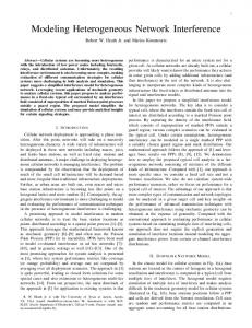
10 how fast does this occur? The kurtosis is a good parameter to use to decide the rate of the process at which the distribution is approximately Gaussian. In probability theory and statistics, (excess) kurtosis is a measure of the “peakedness” of the probability distribution of a realvalued random variable. Higher kurtosis means more of the variance is due to infrequent extreme deviations, as opposed to frequent modestlysized deviations. It is commonly defined as the fourth central moment divided by the square of the variance of the probability distribution minus 3, i.e., £ ¤ E (I − µI )4 C4 κ(I) = − 3 = 2. (23) 4 σI C2 The “−3” term is present to equate the Gaussian distribution’s (excess) kurtosis to zero. Fig. 2 plots the kurtosis of the interference function for various values of the network parameters and helps calculate the N for which its behavior is approximately Gaussian (Kurtosis→ 0). R = 10, B = 10, d = 2, γ = 4 2.5

Kurtosis of the interference distribution

A=2 A=4 A=6

2

A=8

1.5

1

0.5

0 100

200

300

400

500

600

700

800

900

1000

No. of transmitters in the network, N Figure 2. Kurtosis of the interference distribution for different values of A. In each case, the interference distribution converges to a Gaussian.

11

Modeling Interference in Finite Uniformly Random Networks

5.

Outage Analysis

In this section, we determine the outage performance of the binomial network under Rayleigh fading. The outage at the origin is calculated by assuming that the desired transmitter node is located at unit distance from the origin and is transmitting at unit power. The received signal power at the base station due to that node is therefore exponential with unit mean. The outage probability Pr(O) is calculated as Pr(O) = EI [Pr(G/I < Θ | I)] = EI [1 − exp(−IΘ)] = 1 − MI (Θ).

(24)

The probability of success ps is equal to MI (Θ). Fig. 3 compares the success probabilities for the PPP and BPP nodal distributions. We see that the PPP model provides an upper bound on the performance in a binomial network and is not a good assumption to use when there are very few interferers in the network. This is also apparent from Jensen’s inequality and the fact that D is concave. A = 1, B = 5, R = 5, d = 2, γ = 4 1 PPP 0.9

N=3

BPP

0.8

Probability of success

N=5 0.7 0.6

N = 10

0.5 N = 15 0.4 0.3 0.2 0.1 0 0

5

10

15

20

25

30

Threshold (Θ) in dB Figure 3. Comparison of success probabilities for Poisson and binomial networks for different values of N under Rayleigh fading.

12

6.

Concluding Remarks

In this paper, we characterize the interference in a network where the nodes are distributed as a BPP. We derive a closed-form analytical expression for the MGF of the interference at the origin and use it to calculate its cumulants. Under certain specific values of the system parameters, the pdf of the interference is shown to converge to a Gaussian distribution asymptotically as the number of transmitters is increased. We also study the outage behavior of the network and conclude that using the Poisson model in analyses provides an overly optimistic estimate of the network’s performance when the number of interferers is small.

References [1] I. F Akyildiz, W. Su, Y. Sankarasubramaniam and E. Cayirci, “A survey on sensor networks,” IEEE Commun. Magazine, Vol. 40, Iss. 8, pp. 102-114, Aug. 2002. [2] S. Weber, X. Yang, J. G. Andrews, and G. de Veciana,“Transmission Capacity of Wireless Ad Hoc Networks with Outage Constraints,” IEEE Transactions on Information Theory, Vol. 51, pp. 40914102, Dec. 2005. [3] D. Stoyan, W. S. Kendall and J. Mecke, “Stochastic geometry and its applications,” Wiley & Sons, 1978. [4] M. Nakagami, The m-distribution : A general formula for intensity distribution of rapid fading, in W. G. Hoffman, “Statistical Methods in Radiowave Propagation”, Pergamon Press, Oxford, U. K., 1960. [5] A. Ephremides, “Energy concerns in wireless networks,” IEEE Wireless Commun., Vol. 9, pp. 48-59, Aug. 2002. [6] J. Venkataraman, M. Haenggi and O. Collins, ”Shot Noise Models for Outage and Throughput Analyses in Wireless Ad Hoc Networks,” Military Communications Conference (MILCOM’06), Washington DC, Oct. 2006. [7] P. J. Smith, “A Recursive Formulation of the Old Problem of Obtaining Moments from Cumulants and Vice Versa,” The American Statistician, Vol. 49, No. 2, pp 217-218, May 1995. [8] E. Lukacs, “Applications of Fa` a di-Bruno’s Formula in Mathematical Statistics,” The American Mathematical Monthly, Vol. 62, No. 5, pp. 340-348, May 1955. [9] J. Venkataraman and M. Haenggi, “Optimizing the Throughput in Random Wireless Ad Hoc Networks,” 42st Annual Allerton Conference on Communication, Control, and Computing, (Monticello, IL), Oct. 2004. [10] G. Samorodnitsky and M. S. Taqqu, “Stable Non-Gaussian Random Processes: Stochastic Models with Infinite Variance,” Chapman and Hall, 1994. [11] E. S. Sousa and J. A. Silvester, “Optimum Transmission ranges in a DirectSequence Spread Spectrum Multihop Packet Radio Network,” IEEE Journal Selected Areas in Commun., Vol. 8, No. 4, 762-771, Jun. 1990. [12] M. Souryal, B. Vojcic and R. Pickholtz, “Ad Hoc Multihop CDMA networks with Route Diversity in a Rayleigh Fading Channel,” Proc. IEEE MILCOM, Vol. 2, pp. 1003-1007, Oct. 2001.