PHYSICAL REVIEW E 72, 056708 共2005兲
Generating uniformly distributed random networks Yael Artzy-Randrup* and Lewi Stone† Biomathematics Unit, Faculty of Life Sciences, Tel Aviv University, Ramat Aviv 69978, Israel 共Received 17 February 2005; revised manuscript received 28 July 2005; published 16 November 2005兲 The analysis of real networks taken from the biological, social, and physical sciences often requires a carefully posed statistical null-hypothesis approach. One common method requires comparing real networks to an ensemble of random matrices that satisfy realistic constraints in which each different matrix member is equiprobable. We discuss existing methods for generating uniformly distributed 共constrained兲 random matrices, describe their shortcomings, and present an efficient technique that should have many practical applications. DOI: 10.1103/PhysRevE.72.056708
PACS number共s兲: 02.70.⫺c, 89.75.Hc, 89.75.Fb, 05.45.⫺a
I. INTRODUCTION
Characterizing the statistical and mathematical properties of complex networks is an exciting multidisciplinary research area having recent significant impact in the fields of biology, social sciences, and physics 关1–12,15兴. When analyzing real-world systems, it has become common practice to test whether an observed network is different from what one might expect had it been constructed by chance alone—that is, as if all network links were randomly rewired 关4–12兴. This leads us into the arena of null-hypothesis testing where the statistical features of an observed network are compared to those found in an ensemble of representative random networks. This requires a technique for generating an ensemble of random networks with each ensemble member being equally as likely to occur as any other. However, generating uniformly distributed samples from an ensemble of random networks is a complicated procedure as emphasized by the current controversy in the literature 关5–7,10–12,15兴, and the more common algorithms fail to fulfill this criterion. Here we introduce a method that generates uniformly distributed random samples, is more computationally efficient than existing algorithms, is simple to implement, and should have many practical applications. A network is a directed graph whose nodes represent a set of “agents,” with edges linking those nodes that interact in some specified manner. In the study of biological networks, the nodes might represent genes 共/neurons兲 and the links might represent regulation pathways 共/synaptic connections兲. The degree of any given node is defined as the total number of edges it is attached to. A network of N nodes can be fully defined by a 0-1 binary matrix A= = 关aij兴N⫻N with aij = 1 if a directed link exists from node i to j and aij = 0 otherwise. Figure 1共a兲 makes clear the correspondence between a network and its equivalent matrix representation. The row and column sums of the matrix are given by ri = 兺Nj=1aij and N aij, corresponding to the number of outgoing and inc j = 兺i=1 going edges of each node in the network, thereby fully defining the degree distribution of all nodes. The study of 0-1 binary matrices has a long history that is not exclusively confined to networks 关16兴. In ecology, for
*Electronic address:
[email protected] †
Electronic address:
[email protected]
1539-3755/2005/72共5兲/056708共7兲/$23.00
example, they are referred to as presence-absence matrices and summarize the appearance of individuals or species at particular habitats. In the field of island biogeography, rows might represent different species, while columns might represent different sites or islands. If species i is present at site j, then aij = 1 in the binary presence-absence matrix A= ; otherwise, aij = 0. Presence-absence matrices do not necessarily have an equal number of rows and columns, as do matrices describing a network. Computational and statistical methods for analyzing these matrices in biophysics and biological applications have been a source of great friction over the last three decades 关4–7,12–14兴. II. NULL-HYPOTHESIS APPROACH
The null-hypothesis approach is based on a comparison between the observed network and an ensemble of networks that are randomly constructed. By comparing the observed data to “all possible worlds” one can deduce whether or not it is significantly unusual and try to identify those features which are responsible for any nonrandomness. In conducting such tests, three ingredients are essential. First, it is important to precisely define the random null hypothesis. Second an algorithm is required for generating random networks that
FIG. 1. 共a兲 A typical network consisting of five nodes and seven edges. The binary matrix A= = 关aij兴N⫻N on the right fully characterizes the network structure. That is, if an edge is connected between nodes i and j, then the matrix entry is set to aij = 1; otherwise, aij = 0. 共b兲 The feed-forward loop 共FFL兲 is a three-node subgraph with edges connected in the formation shown.
056708-1
©2005 The American Physical Society
PHYSICAL REVIEW E 72, 056708 共2005兲
Y. ARTZY-RANDRUP AND L. STONE
are truly unbiased or “null.” Third, one needs to choose an appropriate test statistic and determine whether the observed score is significantly nonrandom with respect to the distribution of the statistic under the null hypothesis. When defining the null hypothesis it is necessary to allow for realistic constraints that preserve properties of the observed data—properties that might be considered invariant. One common practice that we adhere to in this paper requires conserving the distribution of both incoming and outgoing edges for all nodes in the network—i.e., the degree distribution. This may be achieved by ensuring that each random N and matrix inherits the same row and column sums rគ = 兵ri其i=1 N cគ = 兵c j其 j=1 as the observed system under study. Consider what might arise if the degree distribution of the nodes in the observed network A= was scale free 共with a power-law distribution兲 and the random matrices failed to reflect this degree distribution. In such a case, the null hypothesis might well be rejected for this difference alone, regardless of any unusual characteristics in A= itself. Thus interest centers on generating independent random samples from the full universe U共rគ , cគ 兲 of all 兩U兩 possible matrices which have the same row and column sums. We note that an explicit formula enumerating U共rគ , cគ 兲 has been developed 关17,18兴, which might be useful for estimating sample sizes when conducting null-hypothesis tests. Unfortunately, the formula is awkward to work with since for even relatively small matrices 兩U共rគ , cគ 兲兩 is a large and unwieldly number. III. SAMPLING BY “SWITCHING”
The switching method 关6–9,16兴 is the simplest and best known technique for generating a random sample of matrices in U共rគ , cគ 兲. The method takes advantage of “checkerboard” patterns appearing in a matrix: ]
]
]
... 0 ... 1 ...
... 1 ... 0 ... ]
]
... 0 ... 1 ... ]
]
]
⇔
]
]
... 1 ... 0 ... ]
]
The checkerboard on the left can be switched to its mirror on the right and vice versa without changing the matrices’ row and column sums. Matrices are considered to be “neighbors” if one can be obtained from the other by performing a single switch. Naively, it might be expected that by randomly switching a large number of checkerboard units in the matrix, it is possible to generate a random sample of matrices from U共rគ , cគ 兲. This is the basis of the popular switching method. As each random switch generates a new neighboring matrix belonging to U共rគ , cគ 兲, the technique can be formulated as a Markov chain 共MC兲. It has been proven that any matrix in the universe U共rគ , cគ 兲 can be obtained from any other by some finite number of switches and thus the MC is irreducible 关15,16兴. Being aperiodic, the MC must eventually converge to a unique stationary distribution 关19兴. It should be noted that some network studies exclude the possibility of self-loops—i.e., aii = 0 for 1 艋 i 艋 N in the net-
FIG. 2. An example universe of all 3 ⫻ 3 matrices with row sums rគ = 共1 , 2 , 1兲 and column sums cគ = 共1 , 2 , 1兲 共see also 关5,6,22兴兲. This universe has five members which are connected by a network of checkerboard switches. Some members have a higher probability of being switched to, and therefore when sampling this universe randomly via checkerboard switches, the frequencies of the matrices in the sample are not uniform.
work’s corresponding 0-1 matrix. In such cases it is often necessary to also constrain U共rគ , cគ 兲 to contain only those matrices whose diagonal terms are all aii = 0. This class of matrices is not always irreducible, and therefore the above MC formulation, as it stands, might be thought inappropriate. Nevertheless, we can show that even for such cases, the switching method is valid 关20兴. As an illustration of the switching method consider a universe U共rគ , cគ 兲 of all 3 ⫻ 3 matrices with rគ = 共1 , 2 , 1兲 and cគ = 共1 , 2 , 1兲. This universe has 兩U共rគ , cគ 兲兩 = 5 members, which are presented in Fig. 2. An arrow between two matrices indicates that they are neighbors and that it only requires a single switch to transform from one to the other. If the switching is random, then not all matrices will be visited with the same frequency. Hence the sampling is not uniform 关5,6,15兴. In fact, each matrix will be visited for a time that is proportional to its number of neighbors 关5,19兴. Thus a random walk through U共rគ , cគ 兲 will produce matrices with frequencies proportional to their associated number of neighbors. For the case of Fig. 2, four of the matrices have three neighbors and one matrix has four neighbors. Hence the first four matrices will appear with frequency 3 / 16 and the remaining matrix with frequency 4 / 16. It is possible to calculate the unique stationary distribution of the MC produced by the switching method in a more formal fashion 关15,19兴. Suppose the MC is in the state represented by A= i, a matrix which has a total number of ni checkerboard units or, equivalently, ni different neighboring matrices. Let pij be the probability of moving from matrix A= i to matrix A= j in the MC and set pij =
再
1/ni if matrix Ai and A j are neighbors, 0
otherwise.
冎
共1兲
Take គ = 共1 , . . . , 兩U兩兲 as a probability vector where i is the probability of the MC being in the “state” represented by matrix A= i. As a consequence of the ergodic theorem, i is proportional to the mean amount of time the MC visits the
056708-2
PHYSICAL REVIEW E 72, 056708 共2005兲
GENERATING UNIFORMLY DISTRIBUTED RANDOM NETWORKS
state A= i 关19兴. With each interchange, the probability distribution of the MC is updated by
គ t+1 = គ t P= ,
共2兲
where P= = 关pij兴N⫻N is the transition matrix. For an irreducible and aperiodic MC, the limiting stationary distribution is the * គ * = 共*1 , . . . , 兩U兩 兲, which fulfills probability vector 兩U兩
គ P= = គ ⇔ 兺 *i pij = *j . *
共3兲
*
i=1
兩U兩 nk we find that Taking ␣i = ni / 兺k=1
共4兲 Hence the stationarity condition is satisfied 关Eq. 共3兲兴 and
冒兺 兩U兩
គ = *
គ *S
= 共n1, . . . ,n兩U兩兲
nk .
共5兲
k=1
That is, each matrix is visited in proportion to the number of checkerboards it contains or equivalently its number of neighbors. This has the implication that the switching method cannot generate samples of U共rគ , cគ 兲 that are uniformly distributed. Instead, it is biased—the greater the number of neighbors a matrix has, the more time it will be visited by the MC. For such an MC, the ergodic mean of a chosen statistic f converges to its theoretical mean: ¯f t → គ * under the nonuniS
គ *S,
t→⬁
where t is the length of the MC. form distribution As a check on this we examine a biological example based on the so-called feed-forward loop 共FFL兲 motif 关8,9兴. The FFL motif is a particular three-node subgraph 关see Fig. 1共b兲兴, named aptly because of its hypothesised role in biological networks. There is large body of work 关4,8,9兴 which aims to test whether the FFL motif is significantly more abundant in biological networks than chance would allow for, in which case the FFL might be viewed as evidence for an evolutionary design principle. Hence, as our test statistic, we let f denote the number of FFL motifs in the matrix under investigation. Consider the specific universe U共rគ , cគ 兲 of all 10⫻ 10 matrices with rគ = 共3 , 1 , 7 , 2 , 1 , 3 , 7 , 2 , 5 , 9兲 and cគ = 共4 , 8 , 1 , 4 , 9 , 3 , 1 , 6 , 3 , 1兲. We listed all 兩U兩 = 2214 matrices of this universe and calculated the f score for each of these matrices. It was thus possible to calculate the exact theoretical mean 共គ * = 58.2兲 of f under the stationary distribution S គ *S given by Eq. 共5兲—that is, the mean expected to result from implementing the biased switching method. 共Note that this differs from the theoretical mean for matrices that are uniformly distributed.兲 The expected number of FFL’s per គ *S. Figure 3共a兲 matrix was found to be គ * = 58.2 under S shows this by iterating via the switching method and plotting
FIG. 3. 共a兲 Mean number of FFL’s per matrix generated by the switch, hold, and add methods 共marked with arrows兲, as a function of sample length t 共i.e., number of iterations兲 from U共rគ , cគ 兲, where rគ = 共3 , 1 , 7 , 2 , 1 , 3 , 7 , 2 , 5 , 9兲 and cគ = 共4 , 8 , 1 , 4 , 9 , 3 , 1 , 6 , 3 , 1兲. All three simulations converge to theoretical predictions 共horizontal lines I and II correspond to គ * and គ * , respectively兲. 共b兲 P values S U of the hold and add methods obtained by a one-sampled t test 共see 关28兴兲 between the theoretical mean គ * and the ergodic mean ¯f t as U function of sample length. The significance level 共␣ = 0.05兲 is plotted in black.
the mean number of FFL motifs per matrix as a function of sample size. The MC rapidly converges to the mean គ * = 58.2 FFL’s. S
IV. SAMPLING BY “SWITCHING AND HOLDING”
The so-called Monte Carlo Markov chain 共MCMC兲 hold method 关15,21–23兴 was developed to sample matrices from U共rគ , cគ 兲 uniformly and without bias. The method is based on the way in which a checkerboard unit may be randomly selected in a binary matrix. In this scheme a set of two different rows and columns is chosen at random from matrix A= i. If this set falls on a checkerboard unit, a switch is performed, and the newly generated matrix A= i+1 is registered as the next state in the MC. However, if the set does not fall on a checkerboard unit, the old matrix A= i is again registered as the next state in the MC—i.e., A= i+1 = A= i—and the MC is said “to hold
056708-3
PHYSICAL REVIEW E 72, 056708 共2005兲
Y. ARTZY-RANDRUP AND L. STONE
on” to this matrix. The process is repeated by finding a new random set of rows and columns and either holding onto the old matrix if this trial fails to fall on a checkerboard configuration or moving onto the appropriate neighboring matrix if a checkerboard is found. This contrasts with the switching method where the MC moves to the next state only when a checkerboard is found. In the hold method every trial, checkerboard or not, leads to the creation of a new state. The sample of matrices so produced is thus comprised of a union of chains of repeats of matrices. In the hold method the length of each chain is stochastically determined and there is a correlation between this length and the number of neighbors of a matrix. The fewer the neighbors, the smaller is the probability of finding a checkerboard unit, thereby increasing the chance the MC holds onto the matrix and leading to a longer chain of repeats. The outcome is a negative bias for matrices with many neighbors 共favored by the switching method兲 and a positive bias for matrices with fewer neighbors. The scheme converges to a uniform distribution of frequencies of the different matrices in U共rគ , cគ 兲. To see this formally, define the MCMC transition matrix P= as:
冦
1/QN
matrices Ai and A j are neighbors,
pij = 1 − ni/QN for i = j, 0 otherwise,
冧
共6兲
where QN = 关N共N − 1兲 / 2兴2 is the number of possible sets of pairs of rows and columns one can choose in an N ⫻ N matrix 关24兴. These relations satisfy what are referred to as the detailed balance equations 兵␣i pij = ␣ j p ji其i,j苸U ,
共7兲
where ␣i = 1 / 兩U兩 is the target uniform distribution. Therefore, 兩U兩
兩U兩
兩U兩
␣ j p ji = 兺 ␣i pij = ␣i 兺 pij = ␣i 兺 j=1 j=1 j=1
共8兲
គ * = គ U* = 共1, . . . ,1兲/兩U兩
共9兲
and thus is the limiting stationary distribution 关Eq. 共3兲兴. Hence the hold method leads to a stationary state that is uniformly distributed. This is demonstrated in Fig. 3共a兲 where the average number of FFL motifs 关same U共rគ , cគ 兲 as in the previous example兴 is plotted as a function of sample size for random matrices generated by the hold method. The MC generated by the hold method converges to the theoretical mean គ * = 57.9 as calculated exactly for uniformly distributed U * random matrices គU . A significant drawback of the hold method arises because the probability of repeating or holding onto a matrix is given by pii 关as defined in Eq. 共6兲兴 and is in general very large. An analysis of a wide range of random matrices of different densities shows that typically pii ⬎ 0.87, meaning that in general more than 87% of the trial swaps fail to land on a checkerboard unit. This makes the hold method extremely inefficient and leads to long and redundant chains of copies. As a
FIG. 4. We analyzed N ⫻ N matrices for a range of sizes from N = 5 to N = 100. Matrices were filled randomly with 1’s at different densities, denoted as = 共number of ones兲 / 共N ⫻ N兲. The mean probability of holding was calculated through simulations and tended to decrease with matrix size N but was always large with pii ⬎ 0.87. Notice that for matrices with density and for matrices with density 1 − the mean probability of holding is equal, and so for matrices with = 0.5 the mean probability of being held on to is lowest. For = 0.5 the minimum probability of being held is pii = 0.75 and the maximum is pii = 1, with the mean probability being pii ⬎ 0.87.
result, the number of distinct matrices is greatly reduced, as is the diversity of the random sample of matrices. Thus for the hold method to give a reasonable estimate of the universe of which it is being drawn from, the sample must be very large, as can be seen from Fig. 3共a兲. It is possible to quantify this further. Based on a largescale analysis of simulations we conjecture that the maximum number of neighbors an N ⫻ N matrix has is nmax = 共N / 2兲4, causing pii = 1 − nmax / QN → 0.75 for large N’s 共i.e., the maximum number of checkerboards a 12⫻ 12 matrix can hold is 1296, and thus pii = 0.7025兲. Since the majority of N ⫻ N matrices have much fewer neighbors than nmax, the probability of holding on to them in the MC chain is pii Ⰷ 0.75, and for some cases the probability can be close to 1 共see Fig. 4兲. It follows that the chains of repeats tend to be very long and the variety of different independent matrices sampled is low. As a general example, consider a fictitious population in which each item, once sampled, has a 0.9 probability of being resampled. A sample set assembled from 100 draws would enclose on average only ⬃11 distinct items rather than 100 independent samples. The rest of this sample set would in practice contain repeats of these ⬃11 items. V. SAMPLING BY “SWITCHING AND ADDING”
Here we propose the add method for uniformly generating samples from U共rគ , cគ 兲. The method takes advantage of computational techniques to locate and list all ni checkerboards of each new matrix A= i in the MC. This obviates going through the inefficient search process of randomly stumbling upon sets of rows and columns to locate a checkerboard unit. With the checkerboards located ab initio, the probabilities pij
056708-4
GENERATING UNIFORMLY DISTRIBUTED RANDOM NETWORKS
of the transition matrix in Eq. 共6兲 can be assigned directly and used to make the decision of holding on to the same matrix or advancing to a new one. Each time a matrix A= i is generated by the MC it has a probability of pii = 1 − ni / QN for being reregistered, thus generating a chain of repeats. The chain is composed of a series of failures 共with probability pii兲 corresponding to “holds” and terminates with a single success that corresponds to finding a switch. It thus has a geometric distribution with expected length
PHYSICAL REVIEW E 72, 056708 共2005兲
Their relative frequencies need to be weighted in inverse proportion to their respective number of neighbors. The first four matrices will thus have relative frequencies 1 / 3 ⫻ 3 / 16 and the fifth matrix will have relative frequency 1 / 4 ⫻ 4 / 16. That is, after the weighting, all matrices are equiprobable. VI. COMPARING THE SWITCHING, HOLD, AND ADD METHODS
⬁
Li = 1 + 兺 j共1 − pii兲piij = 1 + pii/共1 − pii兲 = QN/ni . 共10兲 j=1
The add method takes into account long-term averages by directly representing every matrix generated by the MC for a time period 共in terms of iterations兲 that is proportional to its expected hold time Li. That is, when the MC generates matrix A= i, Li copies of this matrix are immediately added to the MC sample. In the long run, the add method must represent matrices in the same proportions as the hold method. In practice, for each matrix A= i generated by the MC, the matching number of neighbors ni is recorded. Once the MC ends its course, these recorded values of neighbors may be retroactively used to determine how many times each matrix should hypothetically be held on to. Seen in another way, according to Eq. 共10兲 each matrix should be weighted by a factor that is inversely proportional to the number of checkerboard units it contains. The result agrees with Zaman and Simberloff 关5兴. This is an intuitively pleasing result since in the switching method Eq. 共5兲 implies that matrices are visited in proportion to their number of checkerboards, but the weighting of the add scheme completely compensates for this effect yielding uniformity in distribution. A potential concern in implementing the add method is that the values of Li = QN / ni in Eq. 共10兲 are generally fractional. If necessary, the Li can always be transformed to integer values by multiplication with a common number C 共e.g., the lowest common multiplier of the ni兲, a procedure that conserves their relative ratios. Conversely, this same reasoning reveals why it is permissible to use fractional 共rather than integral兲 chain lengths Li = QN / ni. For example, when estimating the mean of a statistic f i from a sample with the add method, we use the formula t
¯f = t
t
f
i f iCLi 兺 兺 n i=1 i=1 i t
=
t
CLi 兺 兺 i=1 i=1
1 ni
,
共11兲
where C is some common multiplier of all the ni, such that CLi is an integer for all i. As the QN and C cancel out, the sample mean ¯f t reduces to the familiar “weighted mean,” where each weight correlates to the probability of being sampled, wi = 1 / ni. The weighting scheme of the add method may be easily understood by returning back to the simple example in Fig. 2 where matrices U共rគ , cគ 兲 contains only five distinct matrices.
Figure 3共a兲 provides a comparison of the switching, hold, and add Methods again for the example universe U共rគ , cគ 兲 of all 10⫻ 10 matrices with rគ = 共3 , 1 , 7 , 2 , 1 , 3 , 7 , 2 , 5 , 9兲 and cគ = 共4 , 8 , 1 , 4 , 9 , 3 , 1 , 6 , 3 , 1兲. With respect to the FFL motif statistic f, it is clear that the add method converges far more rapidly to the exact mean គ * = 57.9 than the hold method, U while as we have seen the switching method, being biased, converges to a different mean altogether. A one-sample t test 共see 关28兴兲 was conducted between the exact mean គ * and U sample mean ¯f t for both the hold method and the add method as the MC simulation in Fig. 3共a兲 progressed, giving a p value as a function of sample size 关Fig. 3共b兲兴. In contrast to the add method, the sample mean generated by the hold method stays significantly different from the exact mean even for large sample sizes 共⬎105兲. As some of the key network studies in the literature have relied on the hold method with sample sizes of ⬇1000 matrices, this may be a cause for concern. Figure 3共b兲 makes clear that the sample size of these studies might be underestimated by several orders of magnitude. VII. RUN TIME
The superiority of the add method is due to several reasons. Recall that in the hold method the main motivation for randomly picking rows and columns is not for finding possible checkerboard units 共there are more efficient methods兲, but for determining through trial and error the length of the chains of repeats. In contrast, with the add method each matrix in this scheme is “held” for a period of time that is calculated instantaneously and deterministically, rather than by repeatedly “flipping a coin.” By analytically calculating these values, not only does the add method spare unnecessary computational loops, but it also delivers precise values to act as a weights needed to counteract the natural bias induced by switching. This helps to speed up convergence to stationarity. It has been brought to our attention that the add method belongs to a class of event-induced algorithms, pioneered by Bortz, Kalos, and Lebowitz 关25兴 and has been used in different areas of computational physics 关26,27兴. For example, when simulating the low-temperature relaxation of spin glasses, instead of having an algorithm iterate through many rejections, the waiting time method 关27兴 calculates an expected average waiting time. The algorithm then jumps immediately to its next state at the appropriate moment without iterations. By saving extensive computations, this approach is far more efficient.
056708-5
PHYSICAL REVIEW E 72, 056708 共2005兲
Y. ARTZY-RANDRUP AND L. STONE
* FIG. 5. The distance 储 គU − dគ 共t兲储 关see Eq. 共12兲兴 is used as an index of convergence to stationarity and plotted as a function of sample length t for the three methods based on the universe U共rគ , cគ 兲 of 7 ⫻ 7 matrices 共details in text兲. The switch method converges to theoretically predicted distance 共upper black dashed line兲. The add method converges to zero in a manner similar to ball-urn sampling experiment 共lower gray dashed line; see text兲. The hold method converges towards zero as well, but at a much slower pace.
The rapid convergence of the add method is even more transparent in Fig. 5, plotted for the universe U共rគ , cគ 兲 with rគ = 共1 , 4 , 5 , 5 , 6 , 5 , 7兲 and cគ = 共6 , 6 , 3 , 6 , 4 , 6 , 2兲 which consists of 兩U兩 = 218 matrices. In this figure we plot the distance be共t兲 tween observed 共normalized兲 frequencies dគ 共t兲 = 共d共t兲 1 , . . . , d兩U兩兲 of matrices generated by the MC after t iterations and the * គ *= គU = 共1 , . . . , 1兲 / 兩U兩. We detrue stationary distribution fine the distance as * គU − dគ 共t兲储 = sup 兩Ui − di共t兲兩 储 Ai苸U
共12兲
and plot the distance as a function of the number of matrices generated by the MC. The three different sampling methods were used to generate the vector dគ 共t兲. Convergence to station* គU − dគ 共t兲储 → 0. In Fig. 5, one ary frequencies requires that 储 t→⬁
immediately sees that the switch method fails to converge to a uniform distribution, while the add method converges far more rapidly than the hold method. In order to understand the add method’s convergence rate better we compared it to t balls being dropped randomly into a set of 兩U兩 = 218 urns with equal probability. Let dគ 共t兲 = 共dA1 , . . . , dA兩U兩兲 be the observed 共normalized兲 frequencies of * គU − dគ 共t兲储 as the balls in the urns. Figure 5 plots the distance 储 a function of t and makes clear that the balls converge to a uniform distribution at what appears to be the same rate as the add method. The comparison shows that the convergence of the add method is set in the main by the sampling process itself. VIII. IMPLEMENTING THE NULL-HYPOTHESIS TEST
As an application of the add method consider the matrix M = = 关mij兴N⫻N shown in Fig. 6 belonging to the universe
FIG. 6. Frequency histogram of the distribution of the checkerboard score 共total number of checkerboards兲 in all matrices of U. Matrix M = has 23 checkerboards and is thus considered to be unusual because it lies in the 5% significant region 共in gray兲.
U(共1 , 4 , 5 , 5 , 6 , 5 , 7兲 , 共6 , 6 , 3 , 6 , 4 , 6 , 2兲) of 7 ⫻ 7 matrices. This matrix describes a group of seven scientists interested in seven different topics of research, such that each row in the matrix represents a scientist and each column represents a topic. If a scientist i is interested in topic j, then mij = 1; otherwise, mij = 0. Assuming that some topics attract wider interest than others and that some scientists have more diverse interests, we raise the following question: Is the distribution of interests between scientists a matter of chance, or do these particular seven scientists have some nonrandom pattern of interest? For example, there might be a tendency for scientists to be more drawn towards certain topics or to avoid topics their colleagues are already working on. To the naked eye, this matrix does not appear unusual, and it was thus of interest to subject the matrix to the random nullhypothesis test. We compared the matrix to the entire universe of all possible matrices sharing these constraints 关i.e., the universe U(共1 , 4 , 5 , 5 , 6 , 5 , 7兲 , 共6 , 6 , 3 , 6 , 4 , 6 , 2兲)兴. As a test statistics, we counted the number of times a scientist i1 was interested in topic j1 while another scientist i2 was interested in topic j2, such that i1 was not interested in j2, and i2 was not interested in j1. This corresponds to the number of checkerboard patterns between all scientist i1 and i2. The total number of such checkerboards in matrix M = was found to be n = 23. The distribution of checkerboard scores found in the universe U共r , c兲 as sampled uniformly by the add method is shown as a frequency histogram in Fig. 6. One sees that the number of checkerboards in M = is unusual and significantly overrepresented 共p = 0.04兲, lying in the 5% critical region of the frequency histogram. Thus the interests of the scientists is indeed nonrandom and there is an excess amount of exclusion patterns whereby pairs of scientists tend to avoid working on the same topic. This result may be reproduced by using the exact distribution of checkerboards found from listing all 兩U兩 = 218 matrices. However, if the same test is carried out using the nonuniform switching method to generate a null model, a contrary result is obtained and the number of checkerboards in the above matrix is not significant
056708-6
GENERATING UNIFORMLY DISTRIBUTED RANDOM NETWORKS
PHYSICAL REVIEW E 72, 056708 共2005兲
共p = 0.07兲. Thus the add method gives the correct interpretation while the switching method fails. Finally, we note that we are able to generalize this method so that it is also applicable for networks that lack self-loops 共aii = 0 for all i兲, as will shortly be reported elsewhere.
We gratefully acknowledge the support of the James S. McDonnell Foundation, and thank Professor P. Sibani for helpful suggestions.
关1兴 D. J. Watts and S. H. Strogatz, Nature 共London兲 393, 440 共1988兲. 关2兴 A. L. Barabasi and R. Albert, Science 286, 509 共1999兲. 关3兴 S. Maslov and K. Sneppen, Science 296, 910 共2002兲. 关4兴 Y. Artzy-Randrup, S. Fleishman, N. BenTal, and L. Stone, Science 305, 1107c 共2004兲. 关5兴 A. Zaman and D. Simberloff, Environ. Ecol. Stat. 4, 405 共2002兲. 关6兴 L. Stone and A. Roberts, Oecologia 85, 74 共1990兲. 关7兴 A. Roberts and L. Stone, Oecologia 83, 560 共1990兲. 关8兴 R. Milo, S. Shen-Orr, S. Itzkovitz, N. Kashtan, D. Chklovskii, and U. Alon, Science 298, 824 共2002兲. 关9兴 R. Milo, S. Itzkovitz, N. Kashtan, R. Levitt, S. Shen-Orr, I. Ayzenshtat, M. Sheffer, and U. Alon, Science 303, 1538 共2004兲. 关10兴 O. D. King, Phys. Rev. E 70, 058101 共2004兲. 关11兴 S. Itzkovitz, R. Milo, N. Kashtan, M. E. J. Newman, and U. Alon, Phys. Rev. E 70, 058102 共2004兲. 关12兴 N. J. Gotelli and G. R. Graves, Null Models in Ecology 共Smithsonian Institution Press, Washington, DC, 1996兲. 关13兴 N. J. Gotelli and D. J. McCabe, Ecology 83, 2091 共2002兲. 关14兴 B. F. J. Manly and J. G. Sanderson, Ecology 83, 580 共2002兲. 关15兴 A. R. Rao, R. Jana, and S. Bandyopadhya, Sankhya, Ser. A 58, 225 共1996兲. 关16兴 H. J. Ryser, Combinatorial Mathematics 共The Mathematical Association of America, Buffalo, NY, 1963兲. 关17兴 B. R. Perez-Salvador, S. de-los-Cobos-Silva, M. A. GutierrezAndrade, and A. Torres-Chazaro, Discrete Math. 256, 361
共2002兲. 关18兴 B. Y. Wang and F. Zhang, Discrete Math. 187, 211 共1998兲. 关19兴 S. M. Ross, Stochastic Processes 共Wiley, New York, 1996兲. 关20兴 See http://www.tau.ac.il/lifesci/departments/zoology/members/ stone/stone.html 关21兴 R. Milo, N. Kashtan, S. Itzkovitz, M. E. J. Newman, and U. Alon, e-print cond-mat/0312028. 关22兴 I. Miklos and J. Podani, Ecology 85, 86 共2004兲. 关23兴 G. W. Cobb, www.mtholyoke.edu/courses/gcobb/stat344/ book.html 关24兴 For matrices representing networks with no self-loops, QN = N共N − 1兲共N − 2兲共N − 3兲 / 4 is the number of “legal” pairs of rows and columns one can choose from. 关25兴 A. B. Bortz, M. H. Kalos, and J. L. Lebowitz, J. Comput. Phys. 17, 10 共1975兲. 关26兴 D. T. Gillespie, J. Comput. Phys. 22, 403 共1976兲. 关27兴 J. Dall and P. Sibani, Comput. Phys. Commun. 141, 260 共2001兲. 关28兴 Sequential samples were separated from each other by 1000 switches to prevent dependency. For the hold method the Ct Hi f i / t and the variance is ¯s2t argodic mean is ¯f t = 兺i=1 2 2 ¯ = 关Ct / 共Ct − 1兲兴关共f 兲t − 共f t兲 兴, where Ct is the number of chains in a sample of length t and Hi is the length of each such t t Li f i兲 / 共兺i=1 Li兲 and ¯s2t chain. For the add method, ¯f t = 共兺i=1 2 2 = 关t / 共t − 1兲兴关共f 兲t − 共f¯t兲 兴, such that for the sampled matrix at state i, Li is the expected chain length 关Eq. 共10兲兴.
ACKNOWLEDGMENT
056708-7