IEEE TRANSACTIONS ON GEOSCIENCE AND REMOTE SENSING, VOL. 38, NO. 6, NOVEMBER 2000
2617
Modeling Lidar Returns from Forest Canopies Guoqing Sun, Senior Member, IEEE, and K. Jon Ranson
Abstract—Remote sensing techniques that utilize light detection and ranging (lidar) provide unique data on canopy geometry and subcanopy topography. This type of information will lead to improved understanding of important structures and processes of Earth’s vegetation cover. To understand the relation between canopy structure and the lidar return waveform, a three-dimensional (3-D) model was developed and implemented. Detailed field measurements and forest growth model simulations of forest stands were used to parameterize this vegetation lidar waveform model. In the model, the crown shape of trees determines the vertical distribution of plant material and the corresponding lidar waveforms. Preliminary comparisons of averaged waveforms from an airborne lidar and model simulations shows that the shape of the measured waveform was more similar to simulations using an ellipsoid or hemi-ellipsoid shape. The observed slower decay of the airborne lidar waveforms than the simulated waveforms may indicate the existence of the understories and may also suggest that higher order scattering from the upper canopy may contribute to the lidar signals. The lidar waveforms from stands simulated from a forest growth model show the dependence of the waveform on stand structure. Index Terms—Forest growth model, lidar waveform, three-dimensional (3-D) model.
I. INTRODUCTION
V
EGETATION spatial structure, including plant height, biomass, and vertical and horizontal heterogeneity, is an important factor influencing the exchanges of matter and energy between landscape and atmosphere, and biodiversity of ecosystems [1]. Most remote sensing systems, although providing images of the horizontal organization of canopies, do not provide direct information on the vertical distribution of canopy elements. Laser altimeter systems have been developed to provide high resolution, geolocated measurements of vegetation vertical structure and ground elevations beneath dense canopies. The basis of the method is ranging to the surface obtained by precise timing of the roundtrip travel time of short-duration pulses of backscattered, near-infrared laser radiation. Over the past few years, several airborne and spaceborne lidar systems have been used to make measurements of vegetation. For example, the scanning lidar imager of canopies by echo recovery (SLICER) is an aircraft-based system that has been used to study several different types of forest canopies [2], [3]. The Shuttle laser altimeter (SLA) missions flown in 1996 and 1997 provided laser profile data from vegetation canopies and other surface
Manuscript received July 30, 1999; revised February 22, 2000. G. Sun is with the Department of Geography, University of Maryland, College Park, MD 20742 USA (e-mail:
[email protected]). K. J. Ranson is with Biospheric Sciences Branch, Goddard Space Flight Center (GSFC), Greenbelt, MD 20771 USA. Publisher Item Identifier S 0196-2892(00)07164-3.
features from space. The second mission yielded characteristic differences in laser profiles for different forests [4]. The results of these and other measurements have produced much interest about the potential of this new type of data for remote sensing of forests. This potential is also reflected in the selection of the vegetation canopy lidar (VCL) as the first mission of the NASA’s Earth System Science Pathfinder Program [1]. VCL will provide unique data on canopy geometry and subcanopy topography, which are designed to improve understanding of vegetation canopy structures. The lidar waveform signature has been used to estimate foliage and woody biomass by Maclean [5] and Lefsky et al. [6], and tree height and stand volume by Nelson [7]. These data provide information about the surface elevation, vegetation height, and the vertical distribution of vegetation components. How to derive vegetation physical parameters from lidar data depends on our knowledge of the relationship between lidar waveforms and the spatial structure and optical properties of the vegetation stand. A lidar waveform simulator presents a good tool to study these relationships because in a model, the vegetation scene structure can be exactly described and the misregistration between target and signature, which is always a problem in remote sensing field experiments, can be avoided. Ray-tracing models [8], [9] have been used to simulate waveforms from forest canopies. In forward ray tracing, used in [8], in order to capture enough rays, the aperture size of lidar had to be set to 200 m. The simulation results showed larger higher order scattering than that empirically observed from lidars (e.g., SLICER). Roberts [9] used a reverse ray-tracing model to simulate lidar waveforms from a square footprint. He explored several areas, including the retrieval of tree height and canopy tree height distributions, but the laser pulse across- and along-beam properties were not introduced into the model. In Blair and Hofton’s simulation [10], the waveform of an LVIS footprint was the sum of the elementary pulses reflected from each subpixel within the footprint. The elementary pulse of each subpixel was assumed to be the reflectance at the top surface, which was provided by a small-footprint, first-return-only laser altimeter system. Their simulation results showed that the multiple scattering in the canopy was not a significant contributor to the waveform shape. Models incorporating realistic forest stand structure and lidar properties can be used to investigate the relationship between canopy characteristics and lidar waveform. In this study, the development and implementation of a new three-dimensional (3–D) lidar waveform simulator is discussed. The model was parameterized using measured or modeled forest stand attributes, and the simulated waveforms were evaluated. Section II describes the lidar waveform model. Sections III and IV give detailed descriptions of the parameterization data sets.
0196–2892/00$10.00 © 2000 IEEE
2618
IEEE TRANSACTIONS ON GEOSCIENCE AND REMOTE SENSING, VOL. 38, NO. 6, NOVEMBER 2000
so-called canopy hot spot effect [14]. In the case of exponential cross-correlation and , the hot spot factor becomes (2) The bidirectional gap probability (penetration) in this backscattering case (hot spot) will be
(3) is the density of a one-sided leaf area at depth . is the Ross–Nilson -function, i.e., the mean projec[16]. tion of a unit foliage area at a depth in the direction The bidirectional reflectance factor of the single scattering from and surface area is a canopy layer of thickness
where
Fig. 1. Schematic of lidar pulse and waveform from a single tree with ellipsoidal crown. Also shown is the canopy volume distribution.
Section V describes the model parameterization and simulation procedures. Section VI evaluates the simulated waveforms and Section VII draws some concluding remarks. II. LIDAR WAVEFORM MODEL A. Lidar Waveform of a Single Tree A lidar sends out a short duration laser pulse. The digitizer samples the detector output voltage of returned signal from targets at a certain rate, yielding a waveform for that laser shot [3]. This waveform is a record of return signal as a function of time. The vertical sampling resolution depends on the duration of the digitizer bin. Fig. 1 illustrates a laser pulse and the resulting waveform from a single tree. The tree crown here was modeled as an ellipsoidal scattering medium with half-length and halfwidth . In our previous models [11], the vegetation canopy was treated as a scattering medium (turbid medium). Terminologies such as the volumetric scattering and extinction coefficients were used to describe the optical properties of the medium, and two-way attenuation was used. Because the light source and detector of a lidar are at the same point, lidar is working on a hot spot condition [12]–[15]. According to Kuusk [12], for the leaf canopy, the bidirectional gap probability (BDGP) can be expressed as
(4) where is the area scattering phase function for the canopy [14]. For the geometry used in this study, i.e., a lidar operating in the nadir direction, if the surface of foliage components is , is a constant within Lambertian surface with reflectance will be a constant. and , the canopy volume, the cosines of illuminating and observing angles, are both 1.0. Assuming the canopy is uniform in a thin slab, (4) becomes (5) , and can be functions of canopy depth and The , the horizontal position . The return from a horizontal slab with and thickness at depth , and reaching the surface area 0) can be expressed as top of the canopy ( (6) is the incidence laser intensity. For a uniform ellipwhere soidal crown, the energy returned from a crown slab of thickat and reaching the top of crown can be analytically ness calculated by the following integration:
(1) and are the gap probabilities in illuminating ( ) and viewing ( ) directions, respectively. is the canopy is the hot spot factor. is the angle depth, and between illuminating and viewing directions. When the hot spot factor is 1.0, the expression for the BDGP coincides with the expression for the two-way extinction of turbid medium. and are always at The gap probabilities least partly dependent. This dependence gives rise to the
where
(7) where and are the half length and half width of the ellipsoid is a function of the discrown. The incidence laser intensity tance from the center of the footprint. The time delay of this signal will be the time for light to travel from the lidar to position and back to the lidar. The backscattered signal may also be
SUN AND RANSON: MODELING LIDAR RETURNS FROM FOREST CANOPIES
2619
Fig. 2. 3-D model of a forest stand. Each cell in the model could be specified by its canopy parameters.
presented according to the height from the ground surface. The modeling results will be plotted with respect to the height above the ground surface. The curve at the right in Fig. 1 is the lidar waveform calculated using (7). The vertical distribution profile of the crown volume of the simulated tree was also plotted in the center of Fig. 1. B. Lidar Waveform of a Three-Dimensional (3-D) Forest Stand Ideally, the laser pulse should be of rectangular shape and with infinitesimal duration to ensure accuracy and high vertical resolution. In practice, the laser pulse has a curved shape and finite duration. For example, the laser pulse of SLICER, as described in Section IV, has a pulse width of 4 ns. In this study, we assume a Guassian-shaped pulse defined by a half-power duration and length of tails measured in standard deviations. The vertical resolution of the recorded waveform is 11.2 cm for simulation of SLICER waveforms. Because the pulse width is much larger than the signal digitization interval, every scatterer will produce a series of digitized signals. Each signal bin corresponds to an assumed rectangular pulse with the duration or pulse width equal to the thickness of the crown slab cell. The total signal will be the summation of these bin signals according to their time delay. The intensity of the laser beam across the beam path is also of a Guassian distribution [10] and reduces from the center to the edge of the footprint. from 1.0 to The first step in the modeling process is to build a 3-D scene for a forest stand, as shown in Fig. 2. This requires diameter at breast height (DBH), height, and species for each tree in the stand. The crown shape and crown structure may be determined from these parameters. The 3-D scene is divided into cells according to the required resolution. The cell used in this study was a 0.2 m 0.2 m square slab with a thickness of 0.112 m corresponding to the vertical resolution of SLICER. Every cell within the 3-D forest stand model is assigned to one type of the
crown, gap (between trees), and ground surface cells. The vertical distribution of tree crown volume within a lidar footprint was calculated from its 3-D stand model by summing the volumes of all tree crown cells at the same height from the ground. Let 0 be the top of the stand, and increases downward from the canopy top. If the canopy cell is small, i.e., both and are small, we can assume that the density of scattering medium is constant within this cell, then (6) is the lidar return ). from a cell located at ( from The canopy was divided into layers ( , ), and the lidar pulse was ditop to bottom, with thickness from front to tail, with vided into n narrow pulses ( , ; is the speed of light). If the lidar return duration reaches the subcanopy layer , signal starts when the pulse to hit canopy layer and return the time delay for pulse back toward the lidar will be (without counting the time delay between lidar and upper canopy surface) (8) where is the speed of light. The returned signal will be
(9) where backscattering from a cell at th canopy layer; extinction above this cell; th lidar subpulse. 1) digitizing bins. The lidar waveform is recorded in ( ], [2 , The time delay intervals for these bins are: [0, 2 ], [2 ]. The 4
2620
IEEE TRANSACTIONS ON GEOSCIENCE AND REMOTE SENSING, VOL. 38, NO. 6, NOVEMBER 2000
first interval is when the first (top) canopy layer reflects the first lidar subpulse (front of the lidar pulse). Each lidar subpulse will produce a series of returns as shown in (8). The signals from these subpulses need to be added to proper bins according to the time delay. On the other hand, every column of cells of a footprint will produce a series of signals. The lidar waveform of this footprint is the sum of these signals according to their time delay. Depending on the position of the vertical column of cells within the footprint, a weight is used to modify the laser pulse intensity, calculated from the across-beam distribution
TABLE I CHARACTERISTICS OF SIMULATED FOREST STANDS FROM FOREST SUCCESSION IS THE TOTAL NUMBER OF TREES IN A CIRCULAR PLOT OF MODEL. DIAMETER 25 m. MH IS THE AVERAGE HEIGHT OF ALL TREES IN THE PLOT. MAXH IS THE HEIGHT OF THE TALLEST TREE IN THE PLOT
N
(10) where specifies a vertical cell column within the footprint , is the signal from bin from this column. and When these waveforms are plotted, the signal from the peak of the laser pulse will be registered with the height of the scatterer (Fig. 1). This explains why the scattering (reflectance) from a flat surface (ground) would appear as a Gaussian-shaped waveform with peak at the height of the surface level as shown in Fig. 1 and elsewhere. It should also be noted from Fig. 1 that the peak of the waveform due to the crown return does not coincide with the peak of crown volume vertical distribution. The latter is at the height of the middle of tree crown while the former locates higher. III. FOREST STAND STRUCTURE SIMULATION As discussed above, the 3-D waveform model requires information about every tree in the laser footprint including DBH, height and species. This information can be obtained from field measurements as described in Section IV or through forest growth models described here. A version of the forest model, ZELIG, developed by Urban [17] and described in Levine et al. [18], was used to simulate the successional dynamics of the southern boreal/northern hardwood forest transition zone found at the International Paper’s Northern Experimental Forests (NEF), Howland, ME (45 12’ N, 68 45’ W). The model simulates the annual growth of each tree in a plot whose areal extent relates to the zone of influence of the typical canopy dominant tree or the “gap” that is formed when it dies (i.e., 0.01–0.05 ha). The growth behavior of a species under ideal conditions (e.g., optimal temperature, soil moisture, light, and nutrient availability) is estimated from silvicultural records available at each site. Because soil moisture is considered to be of primary importance in determining the structure (e. g., biomass and species composition) of the forests [19], waterlogging effects were included [20]. To implement the model, site parameters (e.g., soil fertility and monthly values of temperature and precipitation) and autecological parameters (e.g., height and diameter maxima and growth tolerances) were derived from empirical data and published sources. Forest succession on ten types of soil found at the NEF was simulated starting from bare ground [20], [21]. The ZELIG simulations were performed over an area of 30 m 30 m. Model results were recorded at five-year intervals up to 100 years and at 50-year intervals over 250 years. For each simulated stand, the DBH, species, and tree height were recorded for every tree.
Fig. 3. Stem map of four simulated stands (5, 20, 60, and 200 years old). Simulations represent southern boreal/northern hardwood transition forest near Howland, ME. Small circles represent the relative DBH of trees, but not in the scale of the plot axes. The large circle is the lidar footprint (25 m in diameter) for waveform simulation.
Stands simulated on one soil type (Colonel) with moderate soil moisture and fertility were used in this study. Table I lists the characteristics of four stands (age of 5, 20, 60, and 200 years). This modeling approach was also used to parameterize a 3-D radar backscatter model as described by Sun and Ranson [22], [23]. In the present study, trees were randomly positioned within the simulated plot. Fig. 3 shows stem maps of four simulated stands with ages of 5, 20, 60, and 200 years. The small circles in Fig. 3 represent relative sizes of trees, but not at the same scale as the axes. The large circle (25 m in diameter) is the lidar footprint where the lidar waveform signature was simulated. IV. FOREST MEASUREMENT AND AIRBORNE LIDAR DATA At the BOREAS Southern Study Site, Prince Albert, SK, Canada, trees within a 1-ha (100 m by 100 m) mature stand of jack pine were measured. The stem location, DBH, species, and relative canopy position (e.g., dominant, codominant, intermediate, and suppressed) were recorded for each tree in the stand in September 1993. Only trees with a DBH greater than 2.5 cm were measured for a total of 1900 trees. In addition, total
SUN AND RANSON: MODELING LIDAR RETURNS FROM FOREST CANOPIES
2621
TABLE II REGRESSION RELATIONSHIPS FOR CALCULATING TREE PARAMETERS AND THE SCATTERING AND ATTENUATION COEFFICIENT USED IN SIMULATIONS
Fig. 4.
SLICER waveforms extracted from nine 10-m footprints in the 1-ha jack pine forest stand.
height, crown length, and crown width were measured from jack pine trees as part of the BOREAS field activities. The relationships between these parameters and DBH were developed and are listed in Table II. The SLICER instrument was flown onboard a NASA C-130 aircraft on July 29, 1996 over the BOREAS area, including the jack pine site to collect lidar waveforms. Several lines were flown over this site with one traversing the southeast corner of the stem map site. Video tapes of the ground path of the aircraft were reviewed to verify that the correct stand was measured. Several SLICER pixels were extracted from the measured area of the stem map based on pixel latitude and longitude labels. It was not possible to exactly locate the SLICER footprints within
the forest plot, so one-to-one comparisons between SLICER data and the model simulations were not made. However, comparisons of average characteristics of SLICER waveforms and the model results for the same area are still useful. Nine SLICER waveforms within the forest plot were extracted and are shown in Fig. 4. A vertical line in each waveform plot represents the estimated noise floor based on histograms of the lidar return for a pixel. The signal was normalized by the maximum backscattered signal in each waveform, which is from the ground reflectance in all cases. The nine waveforms shown in Fig. 4 are typical of lidar waveforms over forest canopies. The first laser return is from near the top of the crown with later returns coming from successively
2622
IEEE TRANSACTIONS ON GEOSCIENCE AND REMOTE SENSING, VOL. 38, NO. 6, NOVEMBER 2000
Fig. 5. Simulated lidar waveforms for nine footprints in the jack pine stand. The lidar pulse used here was a Gaussian pulse with half-power duration of 4 ns. The two horizontal dotted lines represent (from low to high) the average height of all trees (MH) and the height of the tallest tree in the footprint (MaxH). The tree crown shapes were modeled as hemi-ellipsoids.
lower in the canopy. The rise and fall of the signal with height or the lidar vertical profile reflects the vertical distribution of leaves and branches. The stronger ground return is seen as the spike at bottom of the waveform. Lidar canopy height is the difference between height of the first canopy return and the first ground return. The waveforms in Fig. 4 reveal a canopy with maximum height of about 16 m. The unimodal shapes indicate that the canopy is relatively evenly aged, i.e there is no secondary forest understory. Bimodal profiles suggest the presence of smaller understory trees in the pixel. Fig. 4 shows example of both cases. In a few places within the stand, a 1–2 m tall alder understory is present. Evidence of this can also be seen in Fig. 4 as the small spike near the ground. The averaged waveforms are compared between simulation and SLICER data in the following section. V. SIMULATIONS In the simulations conducted in this study, the following assumptions were made: 1) uniform tree crowns (within a tree crown, the foliage distribution is uniform); 2) uniform ground surface; 3) only single scattering was considered. Three groups of model simulations were performed in this study, as described below. Lidar pulses with Gaussian shape, such as that shown in Fig. 1, were used.
A. Simulation of Lidar Waveforms From a Jack Pine Forest Stand In the first group, nine footprints with a diameter of 10 m were arbitrarily located within the southwest corner of the mapped 1-ha forest stand in the vicinity where SLICER waveforms were extracted. The duration of the simulated laser pulse used was 4 ns, and the vertical resolution of the lidar waveform was 0.112 m. Both parameters are similar to the SLICER instrument parameters [3]. Heights of trees were calculated from DBH using the regression equation developed from field measurements listed in Table II. Crown length and width were calculated based on tree height (Table II). The average height of all trees in the footprint (MH) was also calculated from the data. Tree crown shapes were modeled as cones, ellipsoids, and hemi-ellipsoids (vis Fig. 2). The foliage and ground surface parameters used in the simulations are listed in Table II. The leaf area index (LAI) of this site was measured to be 2.17 in 1994 [24]. From the forest 3-D model, it was found that the total crown volume in a lidar footprint is about 180 and 310 m for conical and ellipsoidal crowns, respectively. The corresponding foliage area volume density (FAVD), calculated from LAI footprint area/crown volume, is 0.95 and 0.55, respectively. We used 0.8 in the simulation. The G-function was assumed to be 0.5 for all cases. The leaf reflectance comes from measurement in [25]. Fig. 5 shows the simulated waveforms for nine lidar footprints when the crowns were modeled as hemi-ellipsoids. The signals
SUN AND RANSON: MODELING LIDAR RETURNS FROM FOREST CANOPIES
2623
Fig. 6. Vertical distribution of crown volume and simulated waveform for the first footprint in Fig. 5. The tree crown shapes were modeled as (a) cones, (b) ellipsoids, and (c) hemi-ellipsoids. The solid curves show the vertical distribution of crown volume, and the dotted curves are the lidar waveforms.
Fig. 8.
Tree height histograms of two simulated forest stands.
Fig. 7. Averaged waveforms from SLICER data (Fig. 4, noise removed) and simulations using different crown shapes.
were normalized by the maximum returned signal in each waveform. The two dashed horizontal lines represent the average tree heights (MH) and the height of the tallest tree in the footprint (MaxH). There are four different types of cells in a 3-D forest stand model: crown, trunk, air, and ground cells. The vertical distribution of tree crown volume within a lidar footprint was calculated from its 3-D stand model by summing the volumes of all tree crown cells at the same height from the ground. Fig. 6 plots the simulated lidar waveforms (dotted lines) for the first footprint in Fig. 5 using cones, ellipsoids, and hemi-ellipsoids as the crown shapes. The vertical distribution of tree crown volume (solid lines) was also normalized by the maximum values and plotted in Fig. 6. Averaged waveforms were calculated for the nine-pixel jack pine simulations for each of the three geometries. The waveforms were added together using the peak signal from the ground surface as reference points. The SLICER waveforms shown in Fig. 4 were smoothed and then averaged. The averaged waveforms (normalized by the peak return) are plotted in Fig. 7.
Fig. 9. Simulated waveforms of four modeled forest stands in Table I. The tree crowns of conifer trees were modeled as cones and those of deciduous trees as ellipsoids. The solid curves show the vertical distribution of crown volume. Dotted curves are lidar waveforms when a Gaussian pulse (10 ns) was used.
B. Modeling Lidar Waveforms Using Forest Stands Simulated From a Forest Growth Model In the second group, the simulated forest stands representing ages of 5, 20, 60, and 200 years (see stem maps in Fig. 3) were used for the lidar model. These modeled canopies represent more complex situations with different tree species, and with wider age and subsequent height distributions. For example, Fig. 8 shows the height histograms of trees within the 25-m footprints from these simulated stands. The lidar simulation results were plotted in Fig. 9. The crowns of conifer trees were simulated as cones, and those of deciduous trees as ellipsoids.
2624
IEEE TRANSACTIONS ON GEOSCIENCE AND REMOTE SENSING, VOL. 38, NO. 6, NOVEMBER 2000
Fig. 10. Crown volume distributions (solid) and simulated lidar waveforms (dotted) of the 200-year old stand when crown shapes were modeled as cones, ellipsoids, and hemi-ellipsoids.
The solid curves represent the normalized vertical distribution of crown volumes. The dotted lines are the simulated waveforms (normalized). Fig. 10 compares the waveforms from a 200-year old stand when the crowns were modeled as cones, ellipsoids, and hemi-ellipsoids. VI. DISCUSSION A. Simulation of Lidar Waveforms From a Jack Pine Stand The simulations shown in Fig. 5 were designed to qualitatively evaluate the model performances. Many factors including the registration, lack of calibration of the SLICER signal, and the uncertainty of lidar footprint position prevented direct comparisons between the measured lidar and simulated waveforms. In addition, there were no direct field measurements of tree heights from this jack pine stand plot. The heights which were used in the simulation were calculated based on DBH using the equation listed in Table II. The heights of trees in this 1-ha stand were in a rather small range of 12–15 m [24]. These can be seen from the differences between the average tree height (MH) and MaxH, which are not as large as those for simulated forest stands in a more temperate climate (Table I). The MaxH very closely matches the first return signal in the simulated lidar waveforms (Fig. 5). For some of the waveforms in Fig. 5, the peak of the canopy return corresponds to the average height of trees in a footprint, but this largely depends on the vertical structure of forest canopies. Different crown shapes lead to different waveforms, especially at the front edge or rising slopes of the waveforms. Fig. 6 compares the waveforms and distribution of canopy volume for the three canopy geometries. The rising slope of the waveforms increases and the peak of the waveforms moves up, when more of the crown volume is in upper layers of the canopy. Because of occultation of the lidar energy by the upper canopy, the retrieval of the vertical distribution of canopy will be more difficult when the canopy material is concentrated in the upper layer of canopy. This can be seen in Fig. 6(b) and(c) for the ellipsoid and hemi-ellipsoid geometries, respectively. Averaged waveforms for the nine-pixel jack pine simulations for each of the three geometries and the averaged SLICER waveforms (normalized by the peak return) are plotted in Fig. 7. By
comparing the rising slopes of the simulated waveforms with that of SLICER one may conclude that the crown shapes of jack pine trees in this plot are likely to be elliptical or hemi- elliptical rather than cones. From Fig. 7, the measured SLICER waveform decays more slowly down through the canopy than the simulations. Rather, all simulations show rapid decay of the waveform. Several parameters used in simulation affect the waveform shapes and may have contributed to these differences such as the vertical distribution of plant material, and the foliage area volume density, and reflection coefficient. The slower decay of the lidar waveform may be due in part to the presence of multiple scattering in the jack pine canopy, which is not considered by the models. But, from the simulations by Blair and Hofton [10], it seems that the multiple scattering is not a significant contributor to the waveforms. The existing understories (scattered alders) then might have contributed to the slow decay of SLICER waveforms, which was not modeled in the simulations. The peak of ground surface return of SLICER was also wider than those simulated. This can be, at least partially, attributed to the roughness of the surface and the presence of some understory in this plot. B. Modeling Lidar Waveforms From Simulated Forest Stands The forest stands modeled for this study represent stands found in the southern boreal/northern hardwood forest transition zone in Maine. Structurally they are much more complex than the 1-ha jack pine in the BOREAS Southern Study Site in Canada, discussed previously. For example, the modeled stands represent various canopy structures including densely five years), and multitier populated small trees (stand age canopy structures (e.g. 20, 60, and 200 years). In addition, the number of trees in each lidar footprint changes significantly as the age of the stand changes (Table I). Tree heights of these forest stands range from 2 m to about 25 m, with a few large trees and many smaller ones (Fig. 8). For this study, tree crowns were modeled as cones, ellipsoids, hemi-ellipsoids, and mixed, i.e., cones for coniferous trees and ellipsoids for deciduous trees. First, we discuss the more general mixed case and present a comparison of the results for the other shapes.
SUN AND RANSON: MODELING LIDAR RETURNS FROM FOREST CANOPIES
Fig. 9 presents the simulation results for the mixed geometry case. Two curves are shown. The curves of vertical distribution of crown volume are plotted as solid lines, and simulated waveforms as dotted lines. Crown distributions and waveform curves were normalized by the maximum value found over all the simulations to enable within and across canopy shape and age comparisons. For the vertical distribution of crown volumes the maximum occurred in the 200-year old stand. The waveform maximum was the ground-return peak in the five-year old stand. The waveforms for the five-year old mixed stand were very similar for the different canopy shapes with a peak for the upper canopy and a peak for the ground return. The waveform for the mixed case [Fig. 9(a)] has a somewhat stronger bimodal shape showing the two reflectance peaks between the crown and ground surface. By checking the species of the trees in this stand, it was found that almost all conifer trees had heights less than 3 m, and all deciduous tress were taller than 3.5 m. The two forest types form the distinct modes in the height distribution (Fig. 8). Using ellipsoids for deciduous trees and cones for conifer trees made the two peaks of crown volume distribution distinct. The lidar waveform from this stand does not show two peaks from the canopy returns. The reflectance peak in the waveform corresponds mainly to the upper canopy of deciduous trees [Fig. 9(a)]. The mixed stands of other ages also show the two-tier crown volume distribution but with different structures. In the 20 and 60-year old stands, the second tier (lower one) is shown to have higher canopy volume [Fig. 9(b) and (c)]. A few emergent trees form the first tier and do not occult the second tier in the lidar beam direction. This can be inferred visually by comparing the waveforms with the canopy distribution curves. The shapes of the waveforms are dependent on the canopy structure, which change with canopy age. For example, the waveform for the upper tier of 20-year-old stand is similar to that from an ellipsoidal canopy (vis. Fig. 1). According to the simulation, the stand has more deciduous (elliptical shapes) at 20 years than for other ages (Table I). As the canopy ages, the successional pattern trends toward more conifer trees (cone shapes). These patterns are revealed in the canopy volume distributions and the waveforms in Fig. 9(c) and (d). In the 200-year old stand simulations, the first tier dominates and occults the second tier. This results in a suppressed waveform in the lower canopy. The effect of canopy shape is further illustrated in Fig. 10. Here, the 200-year-old stand simulations are presented for the three canopy geometries. The waveform for the cone shaped canopy does not exhibit the rapid rising slope of the other two geometries. In each case shown in Fig. 10, the upper tier dominates, but the canopy volume distribution and corresponding waveform are different. These results indicate the type of forest should be known if lidars are to be effectively used to measure canopy volume related attributes such as biomass. The shapes of the waveform can be used to help in this identification process. VII. CONCLUSIONS A 3-D model for simulating lidar waveforms from forest stands of varying geometry and complexity was presented in
2625
this paper. The preliminary comparisons between simulated and measured lidar waveforms show that the model captures the major characteristics of the lidar signature. The simulation results show that the lidar waveform is an indication of both horizontal and vertical structure of forest stands. This work also shows that forest simulators can be used to help explore the effects of canopies of different species and age structure. In our future work, we plan to use detailed tree crown structure (position and optical properties of individual leaf and branch) and radiative transfer modeling to investigate the scattering (single as well as higher-order) and attenuation properties of a crown volume cell as well as a lidar footprint. We will further validate and improve this model when VCL or other lidar data are available. Then the model will be used to study the relationship between forest physical parameters and the lidar waveforms for development of retrieval algorithms. The Earth Science community will be presented with a large amount of new and highly capable data over the next few years with launch of NASA and international platforms. Modeling the interactions of electromagnetic energy with surfaces can lead to better understanding on how to most effectively use this new information. ACKNOWLEDGMENT The authors would like to thank R. Dubayah, University of Maryland, College Park, and J. B. Blair and R. Knox, GSFC, who are investigators in the VCL mission, for discussing ideas for the model and reviewing preliminary drafts of the manuscript. R. Knox also was responsible for the BOREAS jack pine data collection. They would also like to thank D. Harding, GSFC, for providing SLICER data and for help in using the data. Finally, they would like to give their special thanks to the anonymous reviewers. REFERENCES [1] R. Dubayah, J. B. Blair, J. L. Bufton, D. B. Clark, J. JaJa, R. Knox, S. Luthcke, S. Prince, and J. Weishampel, “The vegetation canopy lidar mission,” in Proc. ASPRS Land Satellite Information in the Next Decade II: Sources and Applications, 1997, pp. 100–112. [2] D. J. Harding, J. B. Blair, E. Rodriguez, and T. Michel, “Airborne laser altimetry and interferometric SAR measurements of canopy structure and sub-canopy topography in the pacific northwest,” in Proc. 2nd Topical Symp. Combined Optical-Microwave Earth and Atmosphere Sensing (CO-MEAS’95), April 1995, pp. 22–24. [3] D. J. Harding, J. B. Blair, D. L. Rabine, and K. Still, “SLICER: Scanning lidar imager of canopies by echo recovery instrument and data product description, v. 1.3,” NASA’s Goddard Space Flight Center, Greenbelt, MD, June 2, 1998. [4] J. Garvin, J. Bufton, J. Blair, D. Harding, S. Luthcke, J. Frawley, and D. Rowlands, “Observations of the earth’s topography from the shuttle laser altimeter (SLA): Laer-pulse echo-recovery measurements of terrestrial surfaces,” Phys. Chem. Earth, vol. 23, pp. 1053–1068, 1998. [5] G. A. Maclean, “Estimation of foliage and woody biomass using an airborne lidar system,” Ph.D. dissertation, Univ. Wisconsin, Madison, 1988. [6] M. A. Lefsky, D. Harding, W. B. Cohen, G. Parker, and H. H. Shugart, “Surface lidar remote sensing of basal area and biomass in deciduous forests of Eastern Maryland, USA,” Remote Sens. Environ., vol. 67, pp. 83–98, 1999. [7] N. Nelson, “Estimation of tree heights and stand volume using an airborne lidar system,” Remote Sensing Environ., vol. 56, pp. 1–7, 1996.
2626
IEEE TRANSACTIONS ON GEOSCIENCE AND REMOTE SENSING, VOL. 38, NO. 6, NOVEMBER 2000
[8] Y. M. Govaerts, “A model of light scattering in three-dimensional plant canopies: A Monte Carlo ray tracing approach, Space Applications Institute,” JRC, European Commission, 1996. [9] G. Roberts, “Simulating the vegetation canopy lidar: An investigation of the waveform information content,” Tech. Rep., Univ. College London, London, U.K., 1998. [10] J. B. Blair and M. A. Hofton, “Modeling laser altimeter return waveforms over complex vegetation using high-resolution elevation data,” Geophys. Res. Lett., vol. 26, pp. 2509–2512, August 15, 1999. [11] G. Sun and K. J. Ranson, “Modeling lidar returns from vegetation canopies,” in Proc. SPIE Optical Remote Sensing for Industry and Environmental Monitoring, vol. 3504, Beijing, China, September 15–17, 1998, pp. 67–75. [12] A. Kuusk, “The hot spot effect in plant canopy reflectance,” in Photon-Vegetation Interactions, R. Myneni and J. Ross, Eds. New York: Springer-Verlag, 1991, pp. 139–159. [13] M. M. Verstraete, B. Pinty, and R. E. Dickinson, “A physical model of the bi-directional reflectance of vegetation canopies, 1. Theory,” J. Geophys. Res., vol. 95, no. D8, pp. 11 755–11 765, 1990. [14] T. Nilson, “Approximate analytical methods for calculating the reflection functions of leaf canopies in remote sensing applications,” in Photon-Vegetation Interactions, R. Myneni and J. Ross, Eds. New York: Springer-Verlag, 1991, pp. 139–159. [15] W. Ni, X. Li, C. E. Woodcock, M. R. Caetano, and A. H. Strahler, “An analytical hybrid GORT model for bi-directional reflectance over discontinuous plant canopies,” IEEE Trans. Geosci. Remote Sensing, vol. 37, pp. 987–999, Mar. 1999. [16] T. Nilson, “A theoretical analysis of the frequency of gaps in plant stands,” Agric. Meteorol., vol. 8, pp. 25–38, 1971. [17] D. L. Urban, A Versatile Model To Simulate Forest Pattern: A User Guide To ZELIG, Version 1.0. Charlottesville, VA: Environ. Sci. Dept., Univ. Virginia, 1990. [18] E. R. Levine, K. J. Ranson, and J. A. Smith et al., “Forest ecosystem dynamics: Linking forest succession, soil process and radiation models,” Ecol. Model., vol. 65, pp. 199–219. [19] G. B. Bonan and H. H. Shugart, “Environmental factors and ecological processes in boreal forests,” Annu. Rev. Ecol. Syst., vol. 20, pp. 1–2, 1989. [20] J. F. Weishampel, R. G. Knox, and E. R. Levine, “Modeling soil saturation effects on forest dynamics across a southern boreal landscape,” Bull. Ecol. Soc. Amer., 1999, to be published. [21] K. J. Ranson, G. Sun, J. F. Weishampel, and R. G. Knox, “Forest biomass from combined ecosystem and radar backscatter modeling,” Remote Sens. Environ., vol. 59, pp. 188–133, 1997. [22] G. Sun and K. J. Ranson, “A three-dimensional radar backscatter model of forest canopies,” IEEE Trans. Geosci. Remote Sensing, vol. 33, pp. 372–382, Mar. 1995. , “Radar modeling of forest spatial structure,” Int. J. Remote [23] Sensing, vol. 19, pp. 1769–1791, Sept. 1998. [24] J. M. Chen, P. M. Rich, S. T. Gower, J. M. Norman, and S. Plummer, “Leaf area index of boreal forests: Theory, techniques, and measurements,” J. Geophys. Res., vol. 102, pp. 29 429–29 443, 1997.
[25] E. M. Middleton, S. S. Chan, R. J. Rusin, and S. K. Mitchell, “Optical properties of black spruce and jack pine needles at BOREAS sites in Saskatchewan, Canada,” Can. J. Remote Sensing, vol. 23, no. 2, pp. 108–119, 1997.
Guoqing Sun (SM’99) received the B.S. degree in physics from the University of Science and Technology of China, Beijing, China, in 1970, the M.Sc. in remote sensing from Nanjing University of China, Nanjing, in 1981, and the Ph.D. in geography from the University of California, Santa Barbara, in 1990. He is currently an Associate Research Scientist with the Department of Geography, University of Maryland, College Park, MD, and works with the Biospheric Sciences Branch, Goddard Space Flight Center, Greenbelt, MD. His research interests include land cover and land use change studies from radar and optical remote sensing data, surface height and vegetation spatial structure from Interferometric SAR and lidar, modeling of radar backscatter and lidar waveforms from forest stands, and development of algorithms for forest parameter retrieval from these data.
K. Jon Ranson received the B.S. and M.S. degrees in watershed sciences (now earth resources) and earth resources, respectively, from Colorado State University (CSU), Fort Collins, in 1972 and 1975, respectively. He received the Ph.D. degree from Purdue University, West Lafayette, IN, in 1983. In 1976, Dr. Ranson was employed as a Research Associate in the Earth Resources Department and later the Forest and Wood Sciences Department, CSU. His Doctoral research involved studies of the bidirectional reflectance characteristics of agricultural crops. His graduate studies involved research on the use of Skylab and Landsat MSS data for geologic and forest cover mapping. He spent a year as a Postdoctoral Research Associate and another two years as a Professional Agronomist with the Laboratory for Applications of Remote Sensing, Purdue University. During this time, his research was focused on reflectance behavior of vegetation canopies and microwave backscatter characteristics of crops and trees. In 1986, he joined the Biospheric Sciences Branch, Goddard Space Flight Center, Greenbelt, MD. While there, he continued with bidirectional reflectance studies of forest canopies. Over the past several years, he has also conducted NASA supported radar research including SIR-C/XSAR. In addition to his research activities, he is currently the Deputy Project Scientist for NASA’s EOS Terra spacecraft. Dr. Ranson is a member of the Geoscience and Remote Sensing Society, Sigma Xi, and the American Geophysical Union.