Network Flow Modeling for Flexible Manufacturing Systems with. Re-entrant Lines ..... Our network flow analysis can be used in a pre- processing step to ...
Network Flow Modeling for Flexible Manufacturing Systems with Re-entrant Lines Haitham Hindi and Wheeler Ruml Palo Alto Research Center (PARC), Palo Alto, California 94304 {hhindi,ruml}@parc.com
Abstract— A relaxed version of the process planning problem for flexible manufacturing systems/cells (FMS/FMC) and processing networks, such as flexible flow shops and general job shops, is formulated using a simple extension of multicommodity network flow problems. Our multistage multicommodity network formulation allows for simultaneous routing and resource allocation and also captures the case of re-entrant lines (recirculation). It can be used to perform rapid, albeit crude, explorations of the combinatorial space of possible configurations and failure scenarios. The technique can also provide bounds on the limits of system performance (eg: throughput, link usage, bottlenecks, etc). This can be used to guide the design of robust FMS architectures with high degree of redundancy in machines and routes, as demonstrated in numerical examples. Being a relaxation to the full discrete problem, our method could potentially be used as an admissible heuristic for pruning AI-based planning methods. We demonstrate our approach on a realistic industrial problem.
I. I NTRODUCTION Modern flexible manufacturing systems (FMS) and flexible manufacturing cells (FMC) are highly modular reconfigurable systems that can be composed of hundreds of modules which can be connected in different ways. This leads to an enormous space of possible designs, making the selection of the optimal system architecture a very difficult task. Furthermore, the planning and scheduling of material transport and manufacturing processes can become a major challenge in such complex systems with many possible branches and interconnects. In fact, the two problems of system design and scheduling are not independent. A bad system design could lead to poor schedules, while on the other hand, a inefficient schedule might fail to make the most use of the flexibility and robustness offered by the particular design. Our use of the word “bad” presumes the existence of an optimality criterion, which allows us to measure goodness or badness. Therefore, ideally, one would want to design both the system architecture and the planner simultaneously. In other words, one would like to design an architecture which admits plans that allow for the best possible performance, as measured by the given optimality criterion. In such system optimization problems, when the costs and constraints are convex, one can apply efficient convex optimization to compute a solution [4]. However, in general, planning and scheduling are nonconvex problems, primarily due to the discrete aspects of the components and resource constraints. The flow relaxation approach in this paper is
I
m1
E
N
m2 Fig. 1. A simple re-entrant manufacturing cell viewed as a set of components (I=input, E=exit, mi=machine i) interconnected by a network (N), processing two jobs requiring different sequences of operations: Job1: I→m1→m2→m1→E; Job2: I→m1→E.
a step toward making this multiobjective problem more tractable. Specifically, in this paper, we will present a network flow relaxation for maximizing the steady state throughput of multiclass deterministic processing networks [2], [22] with known fixed processing times, re-entrant lines and no buffers [5], [26], [8]. In such problems there are a set of machines of different types, and a set of different jobs, each requiring a different sequence of operations on the machines, see Fig.1. The objective is to maximize the amount of jobs per unit time that the overall system can produce. We will place particular emphasis on systems with complex routing, where redundancy in machines and routes is designed into the system for fault-tolerance. Such deterministic problems are becoming common today in flexible manufacturing systems [5], [26], [8], where, for example, robots perform sequences of operations on different parts such as milling, spray painting, drilling, etc, all of known fixed duration. This steady state throughput objective arises naturally in applications where the production process is run continually without interruption, or where the jobs are so large that startup transients are insignificant. The steady state throughput objective fits nicely into the network flow framework, which can provide good approximations in situations where the machines are processing large numbers of parts very quickly and deterministically, in a first-in-firstout manner, without complex prioritization or preemption. The deterministic processing times and absence of buffers distinguishes this problem from work on stochastic process-
ing networks [17], [18], [19], [13], [20], or the finite-horizon job-shop problems considered in [6], [2]. It is not the goal of this paper to provide an exact solution to the discrete problem - in general, such problems are NP-complete. For exact solution techniques, see [21], [22], [5], [26], [8], [6], [2] for combinatorial optimization approaches and [1], [12], [25], [24], [11] for discrete search based planning and scheduling methods from constraint programming and artificial intelligence. In fact, we have been successfully using the latter techniques for planning and scheduling in real products for several years [24], [11]. The contribution of this paper is to present a self-contained development of a network flow model for multiclass deterministic processing networks, and to show in detail how it can be applied to problems with complex routing and reentrant lines, a case that was not considered in [27], [15], [26]. We develop an intuitive multistage multicommodity flow formulation, similar in spirit to [27], [15], which can be solved very efficiently using convex optimization. Although, in general, the network flow model does not solve the full discrete problem, it is much faster than the search-based AI methods. Hence, our technique can be used to perform rapid, albeit crude, explorations of the combinatorial space of possible FMS configurations and of failure scenarios. The technique can also provide bounds on the limits of system performance (eg: throughput, link usage, bottlenecks, etc), and hence can be used as a CAD design tool, to guide the design of FMS architectures. It can also be used for load balancing. Finally, we note that since the flow model ignores discretization, it solves a less constrained relaxed problem. Hence it will always produce a bound on performance which is more optimistic than the true optimal. This means that flow model could potentially be used as an admissible heuristic for pruning the AI-based planning and scheduling searches mentioned above [12], [25], [24]. Specifically, we can safely rule out any part of the design space for which the throughput of our network flow model is inadequate, since the throughput of the actual system can only be worse. Our approach is closely related to [27], [15], [26], in the sense that one of our performance objectives is steady state throughput maximization as in [26], while the other is intelligent automated routing as in [27], [15]. At the same time, our approach can be viewed as a special case of the general static planning problem presented in [13] in the context of stochastic networks. This, in turn, has roots in activity analysis, developed by economists in the 1950’s [23], [16], [7]. The dynamic fluid model techniques in [6], [2], [18], [19], [13], [20] can also be viewed as generalizations in which our method is implicitly embedded. See also [10] and the references therein for efforts in the 1980’s to use multicommodity network flows for the traveling salesman problem. However, we have found that the special case considered here very useful in our work on real system designs, so we believe it is worthwhile to describe it explicitly, since it has received relatively little attention in the literature in its own right. We hope that its simplicity and intuitive
g2 g2
g2
g1 m1
g1 m2
m1+m2
g1
Fig. 2. Illustration of the Ricardo-Kantorovich principle: by resource pooling: by means of careful resource management, two machines processing two parts, with different processing capacities for the parts can be more productive as a whole.
interpretation, in terms of multistage multicommodity flows, will make it an appealing and useful tool for practical FMS evaluation and design. II. M OTIVATION A. Ricardo-Kantorovich Resource Pooling In 1817, the British economist D. Ricardo made a remarkable observation which is regarded as one of the fundamental motivations for international trade (ie: resource pooling). Stated concretely, it goes as follows [23]: If two countries are producing two goods, and the countries have different opportunity costs for producing the goods, then by means of specialization and trade, it is possible for both countries to have more of both goods. If the countries have the same opportunity costs, then there will be no benefit from specialization and trade. This is phenomenon is shown in Fig.2. In this figure, the x- and y-axes measure the countries’ capacities for producing the goods g1 and g2, and the shaded regions are the production possibility set for the machines. It is assumed that for each country, the goods trade off linearly. The area above the dashed line in the m1+m2 plot represents the potential gain of resource pooling and judicious management. The entire m1+m2 region is in fact the set sum of the individual production possibility regions of m1 and m2, see [9] for a formal proof of this principle. In other words, by pooling resources and proper management, the countries can be more productive as a whole, without any extra investment in capital or hardware. This principle was rediscovered by Kantorovich in 1939 [16], in the context of flow models for manufacturing systems. In this case, machines replace countries, parts replace goods, and opportunity costs are replaced by processing times. B. Fault Tolerance and Performance Costs Another important motivation for pooling machines, even for single job production, is the idea of graceful degradation in the face of faults. Consider the option of buying a single powerful machine with a certain production capacity or, for the same price, four smaller machines, each with a quarter the capacity of the large one. Clearly, provided that the maintenance cost of the 4-machine system is not higher than
(11)
the single machine system, the consequences of a single failure are much lower for the 4-machine system. Thus robustness is achieved through redundancy. Yet another motivation for networking manufacturing systems is performance cost. It is often the case that a high-end machine with twice the performance of a regular machine costs considerably more than twice as much as the regular one (think of LCD monitors!). So thus there is potential for large savings if low end machines could somehow be easily networked together to work as if they were a single highend machine. Again, this is further motivation for a design tool which allows the rapid exploration of different network architectures.We will show examples of such architectures in section IV.
(12)
sout
m1
sin
m1
I
N
(11)
I
sin
N
E
E
(12)
sout
m2
m2 x12
x11 (13)
(14)
sout
m1
I
N
sin
m1
I
N
(14)
E
E
sout
E
sout
(13)
sin
m2
m2
III. N ETWORK F LOW M ODEL x14
x13
Multiclass processing networks do not immediately fall into the class of standard network flow models, since even at the flow relaxation level, the flow of each job must pass through designated links at each stage. Nevertheless, we will show intuitively and formally in this section, that their relaxations can be viewed as a cascade of standard network flow models, which makes them amenable to linear programming and convex optimization techniques. Our approach uses ideas from [17], [6], [2], [18], [19], [13], [20], [27], [15], [26].
(22)
(21)
sout
m1
sin
m1
I
N
(21)
I
sin
(22)
N
E
m2
m2
x22
x21
A. Flow modeling of multiclass FMS: Intuition Fig. 1 shows a simple re-entrant manufacturing cell viewed as a set of components (I=input, E=exit, mi=machine i) interconnected by a network (N). In this example, two jobs are being processed, requiring the following sequence of operations: Job1: I→m1→m2→m1→E, and Job2: I→m1→E. The re-entrant flow in Fig. 1 (Job1) can be broken up into four constituent flows, one for each stage of the process (x(11) : I → m1 , x(12) : m1 → m2, x(13) : m2 → m1, x(14) : m1 → E), while Job2 can be decomposed into the two flows (x(21) : I → m1, x(22) : m1 → E). These flows are only coupled in two ways: through the network capacity constraints and through equality constraints between the output of one flow to the input of the next, to ensure conservation of the flow, see Fig. 3. Fig. 4 shows how the same technique of Fig. 3 can be easily extended to handle systems with multiple machines of the same type. One can imagine the individual flows being sent to artificial aggregation nodes. The multiple machine case happens in flexible flow shop models [22]. For simplicity, we show just Job1. The flows are again coupled through the network and equality constraints are imposed to ensure that for each component, the input flow at one stage must equal its output flow at the next stage. [Note that the artificial nodes are shown here as a conceptual aid but, because of the equality constraints between stages, we will not need them in our implementation.] Fig. 5 shows the resulting aggregate flows. Just as before, we can easily handle multiple jobs by using more flows.
m1 (21)
I
sin
(11) sin
(22)
N
E
sout
(14)
sout
m2 Fig. 3. Breaking up the re-entrant flow in Fig. 1 into 4 constituent sets of flows of Job1 (x(11) , x(12) , x(13) , x(14) ), and 2 constituent sets of flows of Job2 (x(21) , x(22) ), which are coupled only through the network and machine capacity constraints and through equality constraints between the output of one flow to the input of the next, to ensure conservation of the flow. At the bottom we have the aggregate flow picture.
B. Standard Network Flow Model We now review the standard network flow model [3]. We have a network with N nodes connected by L directed links. For each node n: I(n) is the set of incoming links, and O(n) is the set of outgoing links; sin,n ≥ 0 denotes the flow coming into node n from the outside, and sout,n ≥ 0 is the flow leaving node n to the outside. Let xi ≥ 0 denote flow on link i, and let x be the vector of all the flows. The we can write the flow conservation at each node n as: X
i∈I(n)
xi + sin,n =
X
j∈O(n)
xj + sout,n
(1)
m1
I
m1
m1
m1
m1
N
I
x11
E
I
N
I
m2
m2
m2
m2
m1
Fig. 5.
E
Aggregate flows for the sequence in Fig.4.
m1
I
N
I
m2 x12
I
m2
Aout x + Bout sout
m2 m1
Ain x + Bin sin
Ax + Bout sout − Bin sin
m1
N
E
m2 x13
=
Then, defining the incidence matrix A = (Aout − Ain ) gives m1
I
E
These equations can be written compactly in matrix form by defining the matrices Ain and Bin as follows: � � 1 ; xj ∈ I(i) 1 ; sin,j ∈ I(i) Ain,ij = ; Bin,ij = 0 ; otherwise 0 ; otherwise (2) and similarly define Aout and Bout with I(i) replaced by O(i). The input-output flow balance is now
m2
=
We refer to Bin and Bout as the source matrix and sink matrix, respectively. There will generally be capacity constraints at each link. These can be written in two ways: Let µk denote link-k’s maximum throughput of material per unit time, and let pk = 1/µk denote link-k’s processing time per component. Then we can write either xk ≤ µk or pk xk ≤ 1. The latter will extend more easily to the situation with multiple flows. Thus our overall network flow model in terms of the reduced incidence and source matrices is: Ax + Bout sout − Bin sin = 0 P x � 1 or x � µ x � 0; sin � 0; sout � 0
m1 m1
0
(3)
where µ = (µ1 , . . . , µL ), P = diag(p1 , . . . , pL ) and 1 is the vector of all-ones. I I
C. Multicommodity Network Flow Model N
E
m2 x14
m2
Fig. 4. The technique of Fig. 3 for multiple machines, along with artificial aggregation nodes. The flows are coupled through the machine and network capacity constraints and the equality constraints imposed to ensure that for each component, its input flow at one stage must equal its output flow at the next stage.
The standard network flow model in (3) can be easily extended to handle multiple simultaneous flows on the network, each having its own sources and sinks. This is known as the multicommodity network flow model [3]. Assume that there are F source-destination flows x(i) , i = 1, . . . , F just (i) like the one above, each with its own set of sources sin , (i) (i) (i) (i) sinks sout , and processing times P = diag(p1 , . . . , pL ). These flows are almost independent in the sense that each must satisfy its own flow conservation and nonnegativity constraints, but they are coupled through the shared link
capacities of the network. It follows that the overall network flow model for the multicommodity scenario is [3]: (i) (i) Bout sout
A x(i) + − PF (i) (i) x �1 i=1 P x(i) � 0;
(i) (i) Bin sin
= 0;
i = 1, . . . , F
(i)
(i)
sout � 0;
(i1) (i1)
(i1) (i1)
(ij) (ij)
(ij) (i,j−1)
A x(i1) + Bout sout − Bin sin = 0; A x(ij) + Bout sout − Bin sout
(4)
sin � 0;
the first to get the new conservation constraints:
i = 1, . . . , F
The incidence matrix is the same for the whole graph, but each flow has its own source and sink matrix. If the P (i) are all equal, then we can optionally replace the processing times capacity constraint with the corresponding peak flow PF capacity constraint as in (3) above, ie: i=1 x(i) � µ. But this not always possible to do in general.
j = 2, . . . , Fi (8) Now if there are J multistage jobs, each with its own set of flows x(ij) , j = 1, . . . , Fi , all of which share the interconnection network, then we arrive at our final multistage multicommodity network flow model for a multiple job, multiple stage-per-job, multiple-route scenario is:
A x(ij) +
(ij) (ij) Bout sout
(ij) (ij)
(ij) (ij)
x(ij) � 0;
(ij)
sin � 0;
(ij)
sout � 0;
j = 1, . . . , Fi
∀i, j
(i,j+1)
(i,j)
= sout ,
∀j ≥ 2. (ij)
x(ij) � 0;
= 0;
� 0;
∀i, j ≥ 2 ∀i, j
(9)
sin � 0; ∀i PJ PFi (ij) (ij) x �1 i=1 j=1 P
At this point it is useful to recall the interpretation of the link capacity constraint in (9): since the P (ij) are diagonal matrices, we can write these constraints equivalently at the link level: Fi J X X
(ij) (ij)
pk xk
≤ 1;
k = 1, . . . , L
i=1 j=1
(ij)
(ij)
where pk and xk are, respectively, the processing time and the flow of link k for job i at stage j. So far we have focused on the formulation of the flow constraints but said nothing about the objective function. Basically any objective function that is of interest in network flow optimization is a suitable candidate for our formulation. We mention a few interesting possibilities: • Steady state throughput: as mentioned in the introduction this was one of the primary motivations for our work. The corresponding optimization problem is PJ (i1) max i=1 sin (10) s.t. (9). •
Link utilization: in complex manufacturing cells with highly redundant routes, one might wish to find reasonably sparse flows. Another reason why this might be of interest is for short paths. Both are captured with the same l1 -norm objective [4]. So for example on could minimize the l1 -norm objective subject to the (i) throughput being more than some specified αmin : PJ PFi (ij) k1 min j=1 kx i=1 (11) (i) (i1) s.t. sin � αmin , i = 1, . . . , J; (9).
•
Load Balancing: this can easily be effected either with a term in the objective that penalizes deviation of the flows of the machines from each other, or by imposing constraints that require the flows to be equal or close to each other.
(6)
where Φij is a matrix whose rows are rows of identity corresponding to the link indexes of the machines switched off at that stage. The second feature that must be modeled is the cascading of the stages in each individual job. At each stage, from the second stage onward, the flows on the output links of each final component must equal the input flows to the subsequent stage. This is expressed by the constraint: sin
(ij) sout
∀i
E. The Objective Function
j = 1, . . . , Fi
(5) where A is the incidence matrix of the entire aggregate system, with all the machines included. In addition, two more essential features must be modeled: The first feature is that since, at each stage, we are interested in the flow from one specific set of machines to another specific set, all the other machines must be “switched off”, ie: we must not allow any flow through the other machines in the system at that stage. This is enforced by constraining the flows on the other machines to be zero Φij x(ij) = 0,
−
(ij) (i,j−1) Bin sout
(i1)
We will now introduce the multistage multicommodity network flow model, which allows us to extend the standard and multicommodity network flow models above to the multiple job, multiple stage-per-job, multiple-route, possibly re-entrant scenario. Our development is based on ideas from [6], [2], [18], [19], [13], [20], [27], [15], [26]. Consider a multi-stage job i where we have a set of flows x(ij) , j = 1, . . . , Fi obtained as a result of breaking up the overall process through the components as shown in section III-A. Flow conservation and nonnegativity must hold for each subflow, and they must share the links of the network. Therefore, the flow at each stage is subject to (4) above: A x(ij) + Bout sout − Bin sin = 0; PFi (ij) (ij) x �1 j=1 P
(i1) (i1)
(i1) (i1)
A x(i1) + Bout sout − Bin sin = 0; Φij x(ij) = 0;
D. Multistage Multicommodity Network Flow Model
= 0;
(7)
Using (7) in (5), we can eliminate sin from each stage after
•
Utility, Fairness, Delays: there are several objectives which capture different notions of utility, fairness and expected delays. See [27] and the references therein.
1
2
F. Extensions
IV. E XAMPLES In this section, we present two examples to illustrate our ideas. A. A Simple Two Job System We now present the results of applying our method to the two-job, two-machine example in Fig. 1 with routing Job1: I→m1→m2→m1→E; Job2: I→m1→E. This simple example could be solved by hand. However, it is included here to complete the running example from the earlier section and to show, at the link-node level, the process of breaking up the flows and interpreting the results. The resulting graph topology is shown in Fig. 7. Note that since the jobs are required to pass through the exit link “E”, it must be treated as a third type of machine in our framework too. The processing times on all the links except m1 and m2 were (ij) chosen small enough, pk = 0.1, to ensure that only m1
2
3
m19
4
3
E 4
5
I 1
6
1
7
9
m2 10 8
6
2
2
5
8
10
As pointed out in [27] in the context of communication networks, two extensions are immediately possible. The first extension is that the link capacities themselves could be any concave functions of yet other variables, such as link power consumption, and any convex constraints associated with these variables can easily be appended to (9). The second extension is also inspired by [27]), and this is that it would be interesting to study different solution algorithms such as dual decomposition methods, subgradient cutting plane methods, etc. Another extension is to explore the use of this technique as a heuristic in AI based search methods [1], [12], [25], [24]. Such methods are closely related to branch-and-bound search and essentially enumerate all possible plans (action sequences) and schedules (resource allocation orderings). Efficiency is gained by expanding partial solutions in a ‘best-first’ order defined by a lower bound on the solution objective. Our network flow analysis can be used in a preprocessing step to compute an approximate routing. Possible plans inconsistent with this routing can then be pruned from the search space explored by the AI planner. Note that, because the flow analysis merely approximates the possible actions applicable in the machine, restricting the planner in this way to paths deemed optimal by the flow analysis may result in a suboptimal final production plan. However, the approximation may be very tight in certain applications, and the speed-up in planning time is enormous. If planning must explore a search tree of depth d and breadth b, ie: bd states, then exploring only (b/3)d states may make previously intractable applications feasible. If retaining optimality is critical, the flow analysis results can be used as a ‘node-ordering’ heuristic to focus the planner’s attention on promising actions first while retaining the ability to backtrack to the non-preferred options.
Job−1, Flow−2
Job−1, Flow−1 I 1
1
2
2
3
m19
4
10
9
m2 10 8
1
2
2
3
m19
4
E 4
5
6
I 1
6
1
2
2
Fig. 6.
9
m2 10 8
E 4
6
m2 10 8
6
E 4
6
E 4
6
7
3
m19
4
3
5
5
10
9
7
m2 10 8
6
7
Job−2, Flow−2 3
E 4
5
I 1
6
1
6
2
2
5
7
5
8
7
8
10
9
7
Job−2, Flow−1 I 1
3
Job−1, Flow−4 3
5
7
4
8
7
8
10
m19
5
Job−1, Flow−3 I 1
3
3
m19
4
3
5
5
8
7
10
7
9
m2 10 8
6
7
The four flows of Job1, and the two flows of Job2. Job−1, All Flows I 1
1
2
2
3 m19
4
3
5 E4 5
8 10
Fig. 7.
6
7 9 m2 10 8
6 7
Aggregate flows of Job1. Note that Job1 is a re-entrant job.
and m2 act as bottlenecks. (This was verified by the results of the optimization.) The processing times for m1 (link 9) were set of 0.2 for all stages of job 1, and 0.4 for all stages of job2. The processing times of m2 (link 10) were set to 0.8 for job 1 and arbitrary for job 2, since job 2 must never be routed through m2. (11) The objective was maximization of throughput sin + (21) (11) (21) sin . The resulting optimal flows are sin = sin = 1.25. The individual flows of both jobs are shown in Fig. 6, while the aggregate flows of each job are shown in Fig. 7 and Fig. 8. The link thicknesses are proportional to the flows. The results are easy to understand: Job1 loops through the system, giving rise to twice the flow on the upper path as the lower path (Fig. 7); while Job2 passes straight through, with the same flow in both stages, whose size is consistent with the remaining capacity of m1. Job−2, All Flows I 1
1
2
2
3 m19
4
3
5 E4 5
8 10
Fig. 8.
7 9 m2 10 8
6 7
Aggregate flows of Job2.
6
B. Multimachine Example with Complex Routing
Job−1, Flow−1 m2
In this example, we will show how the graceful degradation mentioned section II-B can been achieved through redundancy and intelligent routing. Although this example may seem somewhat contrived, it is actually a sanitized version of a real application from one of our industry sponsors. Suppose that a single multistage job with the same sequence of operations as job1 above (I→m1→m2→m1→E) is being processed on a manufacturing network with topology shown in Fig. 9. The flow decomposition will be as in Fig. 4 and Fig. 5, except with four instances of each machine type. (Again, the exit link “E” is treated as a third type of machine.) The inputs are on the far left, and the output is the far right. The four machines on the outer perimeter are of type m2; the four machines on the inside are of type m1. For fault-tolerance and production cost, there are multiple instances of each type of machine, with multiple paths into and out of each machine. Note that there are many bidirectional links in this system, represented by pairs of opposing links. (Not all the link labels are visible at this small size unfortunately.) The the network interconnection links, m2 machines, and exit link all have capacities of µ2 = 10. The type m1 machines have a capacity of µ1 = 2.5. The link thickness is proportional to the capacity, hence links of the m1 machines have a quarter the thickness of all the other links. Again, we have chosen the network link capacities to be large, in order to ensure than only m1 machines can act as bottlenecks. Fig. 10 shows the aggregate optimal route, again for throughput maximization. Note that Matlab graphics quantizes the line thickness, so they are only approximately proportional to the flows. The result of the throughput optimization is 5.0 which makes sense, since the total capacity of the bottleneck machines is 4 × 2.5 = 10, but each unit of flow leaving the system must have been processed by an m1 machine twice, thus reducing the total capacity from 10 to 5. We observe that each quadrant runs almost independently performing the m1, m2 and m1 operations locally, and then the flows are combined at the transportation bus in the middle of system. To avoid unnecessary looping or meandering, a small l1 term was added to the max-flow objective. This produces appealing shortest-path like routes. Fig. 11 shows the resulting aggregate routing in the failure scenario, where the top right m2 machine is broken, by severing the link connecting nodes 50 to 49. Nevertheless, the result of the throughput optimization is still 5 - thus achieving the graceful degradation mentioned earlier through redundancy and intelligent routing. Again, the resulting flows are easy to understand. Note that the remaining three m2 machines still have enough capacity to cope with the flow from all four m1 machines. Thus the optimal flow simply processes more m2 flow on one of the remaining working m2’s, namely the one in the upper left. We observe that the lower part of the system is running just as before, but the upper part has done some looping and resource management,
9
21 22
34 33
13
10
36 35 27 28
47 43
m2
17 18 11 23 42 24
m1
38 37
29 41 30 14 19 20 15
48 44
25 26
31 32
49 45
12
41
40 39
114 113
16
50 46
45
101 42 49 50 43 102 103 122 104 116 115
m1
107 109 121 110 46 51 52 47 108
127 123
128 124
105 44 106
118 117
120 119 111 48 112
129 125
130 126
I 165
65
1
1 2
14 13
3
2
4
16 15
3
5 6
18 17
4
20 19
161 33 163
81 82
94 93
83 84
34
96 95
35
85 86
98 97
36 E
168 100 99
67
167 68
169 166
66
5
7 8
9
6
10
7
11 12
8
162 37 164
87 88
89 90
38
39
91 92
40
I 73 77
25
74 78 57 58
63 64
21
59 71 60 26 31 32 27
65 66 51 52
m1
75 79
22
m2
76 80 61 62
67 68
29 30 23 53 72 54
55 56
28
153 157
57
69 70
143 144
24
53
154 158
m1
155 159
137 139 151 140 58 63 64 59 138 145 146
m2
147 148
131 54 61 62 55 132 133 152 134
156 160 141 60 142 149 150 135 56 136
Fig. 9. Topology and relative link capacities for a manufacturing network with multiple machines and redundant routes. (Not all the link labels are visible at this small size unfortunately.)
processing more m2 flow. Note that while the crossing of the flows at node 14 may be unappealing, it is unavoidable in this failure mode. The designer can then easily try other topologies by changing the model, or adding extra links, relying on the optimization to identify the most important ones. As mentioned earlier, this example is based on a sanitized version of a real manufacturing system of one of our industry sponsors. And it was exactly questions such as machine topology, throughput maximization, and failure scenario analysis that were most pertinent during the system architecture and design phase. Running the network flow model presented in this paper was about two orders of magnitude faster than running the discrete planner. Thus many more machine architectures and failure scenarios could be explored, and cases for which the performance of the relaxed network model was poor could be immediately ruled out, since the full discrete planner could not do better. V. C ONCLUSION A relaxed version of the steady state material flow planning problem for flexible manufacturing systems/cells (FMS/FMC) such as flexible flow shops and general job shops is formulated using a simple extension of multicommodity network flow problems. Our convex multistage multicommodity network formulation allows for simultaneous routing and resource allocation, and also captures the case of re-entrant lines (recirculation). It can be used to perform rapid, albeit crude, explorations of the combinatorial space of possible FMS configurations and of failure scenarios. The technique can also provide bounds on the limits of system performance (eg: throughput, link usage, bottlenecks, etc). This can be used to guide the design of robust FMS architectures with high degree of redundancy in routes and machines. Our flow based technique can model the transformation of the components from one form to another, as
Job−1, All Flows m2 10
17 18 11 23 42 24
36 m1 13
27
14
m2 42
37
m1
29 41 30 19 20 15
45
49
43
49 50 43 103 122 104
116
107
46
117
109 121 110 51 52 47
129
123
I 165
65
1
1
3
2
5
3
4
161
33
81
83
34
35
85
36 E
168
167 68
67 169 166
66
7
5
9
6
11
7
8
162
37
87
89
38
39
91
40
I 73 m1 25
57
26
79
m1
59 71 60 31 32 27
57
137
67
66
22
153
58
146
m2 29 30 23 53 72 54
159
139 151 140 63 64 59
54
147 m2 61 62 55 133 152 134
Fig. 10. Throughput-optimal routes and flows for the manufacturing network of Fig. 9.
Job−1, All Flows m2 10
36 m1 13
27
14
m2 broken
17 18 11 23 42 24
37
m1
29 41 30 19 20 15
46
48
43
109 121 110 51 52 47
129
124
I 165
65
1
2
3
5
3
4
161
33
81
34
35
85
36 E
168 67
167 68
169 166
66
7
5
6
9
11
7
8
162
37
87
89
38
39
91
40
I 73 m1 25
57
26
66
22
79
59 71 60 31 32 27
67 m2 29 30 23 53 72 54
153 m1 57
137
58
146
54
159
139 151 140 63 64 59
147 m2 61 62 55 133 152 134
Fig. 11. Throughput-optimal routes and flows for the manufacturing network of Fig. 9, in a partially failed state with the upper-left m2 broken. Yet the system can still run at maximum throughput.
well as their movement from one location to another. Being a relaxation to the full discrete problem, our method could potentially be used as an admissible heuristic for pruning AI-based planning methods. We demonstrated our approach on a realistic industrial problem. Acknowledgment We are grateful to Rong Zhou, Bryan Preas, Lara Crawford, Minh Do, and David Biegelsen for helpful discussions and suggestions, and to Randy Cogill for independently verifying our results and for helping us streamline our formulation. Our computations were done using TOMLAB/CPLEX optimization package for Matlab [14]. R EFERENCES [1] P. Babtiste, C. Le Pape, and W. Nuijten. Constraint-Based Scheduling. Kluwer, 2001.
[2] D. Bertsemas, D. Gamarnik, and J. Sethuraman. From fluid relaxations to practical algorithms for job shop scheduling: the holding cost objective. Operations Research, 51, 2003. [3] D. Bertsimas and J. Tsitsiklis. Intro. to Linear Optimization. Athena Scientific, 1997. [4] S.P. Boyd and L. Vandenberghe. Convex Optimization. Cambridge University Press, 2004. [5] Y. Crama, V. Kats, and J. van de Klundert. Cyclic scheduling in robotic flowshops. Ann. Oper. Res., (96):97–124, 2000. [6] J.G. Dai and G. Weiss. A fluid heuristic for minimizing makespan in job-shops. Operations Research, 50, 2002. [7] G.B. Dantzig. Linear Programming and Extensions. Princeton, 1963. [8] M.W. Dewande, H.N. Geismar, and S.P. Sethi. Dominance of cyclic solutions and challenges in the scheduling of robotic cells. SIAM Review, 47(4):709–721, 2005. [9] A. Dixit and V. Norman. Theory of International Trade. Cambridge University Press, 1980. [10] G. Finke. Practical network methods to solve TSP. In Int. Conf. on Optimization Techniques and Applications, Singapore, 1987. [11] M.P.J. Fromherz, D.G. Bobrow, and J. de Kleer. Model-based computing for design and control of reconfigurable systems. AI Magazine, Special Issue on Qualitative Reasoning, 24, 2003. [12] M. Ghallab, D. Nau, and P. Traverso. Automated Planning. Morgan Kaufmann, 2004. [13] J.M. Harrison. Stochastic networks and activity analysis. In Y. Suhov, editor, Analytic Methods in Applied Probability. American Methematical Society, 2002. [14] K. Holmstrom, A. Goran, and M. Edval. TOMLAB/CPLEX Optimization Software for Matlab. TOMLAB Optimization, http://tomlab.biz, 2005. [15] M. Johansson, L. Xiao, and S. Boyd. Optimal routing and sinr target selection for power-controlled cdma wireless networks. In Modeling and Optimization in Mobile, Ad hoc, and Wireless Networks (WiOpt), 2003. [16] L. Kantorovich. Mathematical methods in the organization and planning of production. Management Science, 6:366–422, 1960 (Russian original 1939). [17] F. Kelly. Reversibility and Stochastic Networks. Wiley, 1979. [18] P.R. Kumar and S.P. Meyn. Duality and linear programs for stability and performance analysis of queuing networks and scheduling policies. IEEE Trans. Aut. Contr., 41:4–17, 1996. [19] C. Maglaras. Dynamic Control of Stochastic Processing Networks: A Fluid Model Approach. PhD thesis, EE Dept, Stanford University, 1998. [20] S.P. Meyn. Workload models for stochastic networks: Value functions and performance evaluation. IEEE Trans. Aut. Contr., 50(8):1106– 1122, 2005. [21] M.L. Pinedo. Scheduling Theory Algorithms and Systems. 2002, Prentice Hall. [22] M.L. Pinedo. Planning and Scheduling in Manufacturing and Services. 2005, Springer. [23] D. Ricardo. On The Principles of Political Economy and Taxation. John Murray, Albemarle-Street, London, 1817. [24] W. Ruml, M.B. Do, and M.P.J. Fromherz. On-line planning and scheduling in a high-speed manufacturing domain. In Proceedings of the Fifteenth International Conference on Automated Planning and Scheduling (ICAPS-05), 2005. [25] S. Russell and P. Norvig. Artificial Intelligence: A Modern Approach. Prentice Hall, 2002. [26] T-.Y. Wang and Y-.L. Chen. Applying the network flow model to evaluate an FMC’s throughput. Int. J. Prod. Res., 40(3):525–536, 2002. [27] L. Xiao, M. Johansson, and S. Boyd. Simultaneous routing and resource allocation via dual decomposition. IEEE Trans. on Comm., 52(7):1136–1144, July 2004.