Citation: CPT Pharmacometrics Syst. Pharmacol. (2018) 7, 288–297; doi:10.1002/psp4.12299 All rights reserved
C 2018 ASCPT V
TUTORIAL
Many Flavors of Model-Based Meta-Analysis: Part II – Modeling Summary Level Longitudinal Responses Martin Boucher*and Meg Bennetts
Meta-analyses typically assess comparative treatment response for an end point at specific timepoints across studies. However, during drug development, it is often of interest to understand the response time-course of competitor compounds for a variety of purposes. Examples of such application include informing study design and characterizing the onset, maintenance, and offset of action. This tutorial acts as a ‘‘points for consideration’’ document, reviews relevant literature, and fits a longitudinal model to an example dataset. CPT Pharmacometrics Syst. Pharmacol. (2018) 7, 288–297; doi:10.1002/psp4.12299; published online 20 April 2018.
Part I of the model-based meta-analysis (MBMA) tutorial highlighted the critical importance for companies developing drugs to understand the key safety and efficacy attributes of other compounds, either on the market or in the pipeline.1 The focus of many articles is to present study results based on primary and secondary end points in which more often than not, these end points will be landmark, for instance at a specific timepoint or an event, such as “end of study.” However, it is common for published study results to also include time-course information, usually in a graph or a table, thus providing a much more informative view of the data than a landmark end point. Fitting models to the time-course of response can have many benefits especially in the learning phase of development (typically phase II) but it can also impact the confirmatory stage (typically phase III). Having clear research questions for a drug’s development will help decide whether longitudinal modeling will add value for a project team. A benefit of modeling time-course data is to understand the full response profile for different compounds and/or placebo. This includes the onset of action, maintenance of effect, and any offset of response. Two competing drugs may have similar efficacy at week 6 but, with all other things being equal, a compound with a quicker onset of action is likely to be preferred by patients. A response that is maintained over a significant time-frame should be more meaningful than a response at a single point in time. A second example is when previous proof of concept (POC) trials in a specific indication were typically 6 weeks in length but longitudinal data from historical trials of another mechanistically similar drug, to the one in development, demonstrate that a strong response can be shown as early as week 2. This could result in designing shorter POC trials in the future for this indication. In addition, following the readout of a short-term POC study, it is useful to predict a response in a study of longer duration. Wang et al.2 looked at how predictive a short-term result (3 months) was of a longer-term response (6 months) using a longitudinal model for responder rates. By using existing time-course information from similar types of
compounds reported in the literature, a scalar between two timepoints could be estimated and applied to the POC study result to generate the predictions for a future longer study design. Depending on the types of models used, interpolation can be used to get estimates at timepoints that have been little studied (or not at all). This will be discussed further, later in the tutorial. First, the aim of this tutorial is to review previous publications on longitudinal meta-analyses. Second, we wish to highlight important considerations in modeling time-course data. Finally, an maximum effect (Emax) model is fitted to an example osteoarthritis (OA) pain dataset using a selection of commonly used software in the pharmaceutical industry within (but not exclusively) Clinical Pharmacology. Landmark meta-analyses at selected timepoints will also be compared with the longitudinal model estimates. The dataset, model code, and outputs from the modeling will be provided in the Supplementary Materials. The primary focus here is on modeling aggregate data and, hence, MBMA of individual patient data (IPD) or combined aggregate data/ IPD data will not be covered. REVIEW OF LITERATURE COVERING LONGITUDINAL MBMA The number of published articles on longitudinal metaanalyses, particularly for methodology development, is relatively small, as is the case for MBMA methodology in general. However, there has been a fairly consistent rate of such publications during the last 10 years, particularly with regard to the application of MBMA methods. In terms of methodology, several articles have focused on the issue of accounting for residual correlations between timepoints, comparing the different approaches used to account for them, and the consequences of not doing so. Ishak et al.3 fitted a variety of models to deep-brain stimulation data from patients with Parkinson’s disease, all of which accounted for the correlations between timepoints within a study treatment arm. The article concluded that
Department of Pharmacometrics, Pfizer Ltd, Sandwich, Kent, UK. *Correspondence: Martin Boucher (
[email protected]) Received 6 December 2017; accepted 19 March 2018; published online on 20 April 2018. doi:10.1002/psp4.12299
Part II – Modeling Summary Level Longitudinal Responses Boucher and Bennetts 289
accounting for these correlations could result in a better model fit and more precise parameter estimates. Similarly, Musekiwa et al.4 discussed and compared different covariance structures when fitting linear mixed effect models to an example dataset of 17 trials, which compared the combination of radiotherapy and chemotherapy with radiotherapy alone. With more of an MBMA focus, Ahn & French5 expanded on the work by Ishak et al.3 to nonlinear timecourse and dose-response models with an emphasis on how compound symmetry correlations can be accounted for using the NONMEM software package and then, quantifying the resulting bias of not accounting for this correlation appropriately through an extensive simulation exercise. Although Emax and exponential models are common for fitting time-course in the Clinical Pharmacology arena, there are plenty of alternatives. Jansen et al.6 presented a network meta-analysis in which the time-course for OA pain was incorporated using fractional polynomials. These are flexible nonlinear models and are an extension of polynomial models.7 Whereas their flexibility is certainly an advantage, the parameter estimates themselves may not be so useful or intuitive in the same way that Emax or ED50/ET50 parameters tell us about relative maximal effects or potency/onset of action. Luu et al.8 used a cosine model to reflect circadian intraocular pressure of patients with glaucoma or ocular hypertension. There are also examples of authors transforming discrete measurements, such as responder rates or bounded mean pain scores, into logit space and then applying nonlinear models.9,10 There are several other examples of applications of longitudinal MBMA that we do not discuss here but a table of these is provided in the Supplementary Materials Table S1, which includes the disease area, end points, and types of longitudinal models fitted. Additionally, further examples are referenced separately in the discussion section. IMPORTANT CONSIDERATIONS WITH LONGITUDINAL MBMA Time: Continuous variable or factor Clinical pharmacologists conventionally consider “time” and “dose” to be continuous variables, as demonstrated by the routine use of Emax or exponential models. These models readily support interpolation and, less commonly, extrapolation for future study prediction. Repeated measures analysis, in which time is treated as a factor, is more commonly used by statisticians to be used with good effect to describe the data at each timepoint with fewer assumptions. In summary, treating time as continuous is advisable when the goal of the analysis is broader than purely description, such as prediction, clinical trial simulation, or to reflect underlying pharmacology. Different imputation methods One of the major challenges with MBMA longitudinal data is that published summary level data are analyzed and reported in disparate ways across articles. Different articles may summaries different timepoints: some with a rich timecourse of many results and others with just a baseline and end of study result. Access to original reports, from
company or regulatory websites, may be used to fill in unpublished timepoints, if available. Identifying the method used by each publication to handle missing data at each timepoint and then determining how to account for any differences can be a major undertaking.11 The end point time-course data in plots or tables may not be based on the same imputation method as the final end point analysis. For example, observed case (OC; no imputation) time-course data for the measure of interest can be plotted alongside the end of study statistical analysis result for which an imputation method has been applied, such as: last observation carried forward (LOCF), worst observation carried forward, baseline observation carried forward (BOCF), and multiple imputation, among others.12 End-point relationships are likely to vary over time depending on the imputation method used. However, this may not be important if we are only looking at early timepoints in which dropout is likely to be minimal. However, as the length of the study increases, differences in imputation method will become more of an issue. Access to IPD can reduce these differences by re-imputing summary level data using the most relevant method. However, for published data this is rarely possible and other methods accounting for these differences will need to be considered. One straightforward approach would be to only include articles with an imputation method that matches the one planned for use in the specific drug development program the MBMA is aimed to inform. Alternatively, multiple independent MBMAs could be performed, one for each of the different imputation methods. However, this would be both time-consuming and not an efficient way to use the full dataset. A further approach might be to combine all the data from different imputation methods and then fit a covariate to estimate the effect for each method (e.g., LOCF vs. OC vs. BOCF). In this covariate approach, some studies may report summary data for more than one imputation method; in this case, correlation between endpoints/ imputation methods, within trials, would also need to be considered. Outcome reporting bias The issue of outcome reporting bias needs careful consideration and arises when some or all of the included publications do not present the full time-course results of their underlying studies.13 It is important to understand which studies are contributing to the information at each timepoint and creating a table to show how this would be instructive. Published plots will not always present the corresponding SEs of the means and, when they do, it may be difficult to digitize these accurately if the plots are of poor quality or the points/bars overlap. Digitization of these plots also introduces another source of transcription error. When OC data are presented on a plot without precision estimates and/or sample size information (which change over time when there is dropout), the analyst is left with the dilemma of how to weigh the residuals. Correlations between timepoints within treatment arms For time-course models, it is important to acknowledge that mean responses for a study arm will be correlated between www.psp-journal.com
Part II – Modeling Summary Level Longitudinal Responses Boucher and Bennetts 290
timepoints because these responses include the same individuals, subject to dropout and imputation method. Ignoring such correlation could lead to over precise estimates, bias, and more weight assigned to studies with many timepoints over those with few timepoints. It should be noted that correlations at the summary level may be different to those at the IPD level. If correlation is accounted for using study-level and armlevel random effects (one of the approaches outlined in Ahn & French5), then arm-level effects should be nested within the corresponding study-level effects. The NONMEM version 7.3 software package has the option to include more levels of random effects with such nesting compared with previous versions so that setting up compound symmetry is now much easier.14 To implement in R, the nonlinear mixed effect (NLME) function for fitting NLME models has options for defining different correlation structures (e.g., compound symmetry, autoregressive (AR(1) etc)). The NONMEM version 7.3 also allows the use of AR residuals. In BUGS, compound symmetry can be set up either using the approach outlined in Ahn & French,5 which is discussed in the previous section, or by constructing the residuals in matrix form. The latter method is not straightforward when there are trials with different “dimensions” of timepoints. As a recommendation, we suggest that, once the best available structural model has been chosen and fitted, the time-course of residuals are plotted by study and treatment. If runs of positive or negative values are observed within a study treatment arm, then this would suggest that there is still some residual correlation that needs to be accounted for. Compound symmetry would be a good starting point, only proceeding to other methods, such as AR, if necessary. Residual weighting Ideally for mean data, residuals should be weighted by the precision of the mean (the reciprocal of SE2 5 1/(SE2) 5 1/ (SD2/N)). We recommend that available SDs over time are routinely plotted, as part of the exploratory analysis, to assess potential models for SD imputation, if required. This can also be a useful way of identifying unusual values (such as a SE being reported as an SD or vice-versa). There are many approaches to deal with missing SDs but Boucher used an NLME model to impute missing SDs over time for this type of data.15 Wiebe et al.16 provided a nice review of methods that have been used to impute missing variance data. If, however, the number of missing SDs is high then it may be more appropriate to weight using the sample size. This makes an assumption that the within study SDs are the same across all studies and timepoints, which may not be a realistic assumption depending on the design and population characteristics of the included trials. Covariate effects In traditional meta-analyses, the term “meta-regression” is often used to describe the fitting of covariates, although “covariate analysis” is a more commonly used phrase in Clinical Pharmacology. Compared with landmark metaanalyses, there are potentially more parameters to which CPT: Pharmacometrics & Systems Pharmacology
covariates could be fitted when modeling longitudinal data. However, the limitations of covariates at the summary level remain the same, namely: small ranges of observed values at the mean level; inability to use the summary level covariate to make inferences at the patient level, due to ecological bias; and the often small numbers of studies involved in an MBMA.17 Plotting the relationship between endpoint and potential covariates is the first step to identifying those to take forward into a covariate analysis. Between-study variability The ability to get a good estimate of between-study variability will largely depend on the number of trials that are available for the analysis. If there are insufficient studies to get a good estimate, then one option would be to take the Bayesian approach and use a prior based on a similar analysis of different data. As will be seen in the example, longitudinal models provide scope for more than one random effect. In the first tutorial, Q and I2 were discussed as approaches to assess between-study variability along with reasons why they may not be particularly useful. They have not been adapted for MBMA, as far as we know, and we would not recommend their use for these longitudinal models. Model diagnostics There are a much greater number of potential diagnostics that can be carried out on a longitudinal model than for a landmark model. Broadly speaking there is residual-based and simulation-based diagnostics. Examples of residualbased diagnostics are weighted residuals over time, weighted residuals vs. predictions, and a histogram of residuals (or other plots that assess the distributional assumption for the residuals). A common simulation-based diagnostic is the visual predictive check, which assesses how well the model describes the observed data. The mean and quartiles of the simulated data are compared with the mean and quartiles of the observed data. These can be produced using PsN.18 Normalized prediction distribution errors (NPDEs) are one of the newer simulation-based metrics used to evaluate NLME models and when the model is a good fit of the data, the NPDEs would be expected to be distributed N(0.1).19 NPDEs can be produced in NONMEM version 7.3 by inserting “NPDE” in the table line of the command file. There is also a library in R (npde) that can produce these. EXAMPLE DATASET: WESTERN ONTARIO AND MCMASTER UNIVERSITIES PAIN IN OSTEOARTHRITIS In order to understand the time-course characteristics of naproxen in OA, internal clinical study reports and publically available literature were searched to find relevant doubleblind, randomized, placebo-controlled parallel-group studies. All trials included both naproxen and placebo treatment arms. The endpoint of interest was the Western Ontario and McMaster Universities (WOMAC) pain score, which is the same as the example used in part I of this tutorial, except that now, time-course information has been included. Study
Part II – Modeling Summary Level Longitudinal Responses Boucher and Bennetts 291
Figure 1 Mean Western Ontario and McMaster Universities (WOMAC) pain over time for naproxen and placebo split by study design.
characteristics are presented in Supplementary Table S2. For “flare” trials, subjects were washed out of their pain medications and were required to have a predefined increase in pain (a flare-up) to be eligible for randomization. Of the 18 trials included in this MBMA, 12 were flare designs and 6 were not. Research questions As emphasized in the first tutorial, formulating clearly defined research questions will lead to a more focused and efficient piece of work and avoid time-consuming “fishing” exercises. In addition to comparing the longitudinal methodology with landmark estimates, the research questions for this WOMAC pain example are: How does the onset of action and maximal effect compare between naproxen and placebo? Note: a quick onset of action could result in the possibility of running a shorter “first-in-patient” trial. 1) Does a flare design have any impact on treatment effect? Is there an advantage/disadvantage to using such a design in terms of the resulting treatment difference estimate? Note: flare designs are more selective and recruitment could take longer, therefore, if there is no advantage in this design then there is potential to complete the study sooner. Both of
these questions speak to specific model parameters that will be described in the next section. METHODS Figure 1 presents the mean WOMAC pain scores across time stratified by treatment (naproxen or placebo) and design (flare or nonflare). This plot shows a quick onset of action (