Ecological Modelling 169 (2003) 103–117
Modeling the density–area relationship in a dynamic landscape: an examination for the beetle Tetraopes tetraophthalmus and a generalized model Stephen F. Matter∗ Department of Biological Sciences, University of Cincinnati, Cincinnati, OH 45221-0006, USA Received 29 November 2002; received in revised form 17 June 2003; accepted 16 July 2003
Abstract The relationship between local population density and habitat area is an important factor in spatial population ecology. I examined how density dependence in the growth of local insect populations and their host plant patches, combined with patch birth and death, and insect dispersal affect the density–area relationship. I constructed a simulation model to examine the relationship for an insect herbivore, Tetraopes tetraophthalmus, inhabiting patches of its host plant, Asclepias syriaca. Given the observed growth of insect populations, patch growth, dispersal of insects, and change in the number of patches within the landscape, the model predicts that T. tetraophthalmus density should decrease with increasing A. syriaca patch size. The model also predicts moderate amounts of temporal variation in the relationship. A more general insect herbivore-host plant model was also developed to extend the results. The general model shows that density dependence in patch and insect population growth rates have large effects on the density–area relationship. The density–area relationship was strongly affected by density dependence in insect growth. Increasing density dependence in insect growth caused insect density to decrease with increasing patch size. Temporal variation in the relationship was most strongly affected by density dependence in patch growth. Variation in the density–area relationship increased as density dependence in patch growth increased. The results of this study show that density–area relationships can be variable and are not necessarily a species-specific trait. Application of density–area relationships, especially in dynamic landscapes, need to be aware of and account for factors that affect the size and number of patches as well as growth and dispersal of the target populations. © 2003 Elsevier B.V. All rights reserved. Keywords: Asclepias; Density dependence; Dispersal; Individuals–area relationship; Metapopulation; Patch
1. Introduction How population density relates to habitat size is an important consideration in the research of spatial population dynamics. Reviews of this topic, the density–area relationship (also called the individuals– area relationship; Schoener, 1986), have shown pat∗ Tel.: +1-513-556-9713; fax: +1-513-556-5299. E-mail address:
[email protected] (S.F. Matter).
terns of increasing, decreasing, and constant density relative to habitat area (Bowers and Matter, 1997; Bender et al., 1998; Connor et al., 2000). Despite the diversity of relationships, in general, population densities tend to increase with patch or habitat area (Connor et al., 2000; but see Gaston and Matter, 2002). The relationship between population density and habitat size underlies basic ecological theory and is pertinent to conservation issues (Haila, 1988; Andrén, 1994; Gaston et al., 1999; Connor et al., 2000; Matter, 2000;
0304-3800/$ – see front matter © 2003 Elsevier B.V. All rights reserved. doi:10.1016/j.ecolmodel.2003.07.002
104
S.F. Matter / Ecological Modelling 169 (2003) 103–117
Gaston and Matter, 2002). From a phenomenological perspective, the relationship affects population dynamics and community patterns. Within a metapopulation, increasing or decreasing population density with area results in individuals being clustered into large or small patches, respectively. This clustering changes the relative importance of different sized patches, altering predictions of metapopulation dynamics and community patterns (Matter, 2000, 2001a). Similarly, local populations of the same size, but within networks with different density–area relationships can show different dynamics (Matter, 1999). The density–area relationship has been proposed as a tool for reserve design, particularly in relation to the single large or several small (SLOSS) debate (Connor et al., 2000). The reasoning here is simple. For species that show increasing density with area, a large reserve will contain a greater abundance of individuals than any number of smaller reserves summing to the same size (Matter, 2000). As a null expectation, density should not vary with habitat area (Haila, 1988; Bowers and Matter, 1997). Several mechanisms have been offered to explain deviations from this expectation. Root (1973) proposed that insect density should increase with increasing patch size if emigration rates are greater from small patches, and immigration rates and residence times are greater for large patches. Several studies have shown dispersal rates consistent with density patterns (Raupp and Denno, 1979; Kareiva, 1985; Bach, 1988), supporting a dispersal-based mechanism. However, behavioral models indicate that immigration rates may not be expected to increase with habitat area (Bowman et al., 2002). The enemies hypothesis predicts that predation rates are higher on small patches than on large patches producing positive density–area relationships (Denno et al., 1981; Risch, 1981). Habitat quality may vary with patch size producing increasing or decreasing density with area (Bach, 1988; Hanski, 1994; Matter, 1997). If habitat quality varies within patches such that the edges of patches are of higher or lower quality, the density–area relationship may vary with the perimeter to area ratio (Bowers et al., 1996; Bender et al., 1998; Haddad and Baum, 1999). Bowers and Matter (1997) proposed that mechanisms producing density–area relationships may depend on spatial scale. Habitat selection at small spatial scales may produce negative relationships
if territorial individuals preempt non-territorial individuals from larger habitats. Positive relationships may arise at broader spatial scales through colonization-extinction dynamics. Here, small patches would support smaller populations on average due to their higher frequency of extinction. Density–area relationships may also result from methodological problems such as the mis-estimation of habitat area for edge species (Bender et al., 1998) or the inclusion of increasing amounts of non-habitat with increasing size of census areas (Smallwood and Schonewald, 1996; Gaston and Matter, 2002; Matter et al., 2003). Despite the importance of and attention given to density–area relationships, previous research has neglected two key aspects. First, density–area relationships may show temporal variability. Most empirical relationships have been demonstrated only over a single generation, which precludes between generation effects and ignores temporal variation in the relationship (Matter, 1999). Second, most investigations have ignored any effect of variability in the landscape, which may be significant for insect herbivores inhabiting patches of their host plants. This research investigates the magnitude of and temporal variation in the density–area relationship. I focus on herbivorous insects inhabiting patches of their host plant in a dynamic landscape. It is unclear how the relationship in a dynamic landscape compares to that for static systems, and how change in the landscape affects density–area relationships. Most models of spatial population dynamics assume that landscapes are stable (Kareiva, 1983; Pulliam, 1988; Hanski, 1994), or that variability occurs over large spatio-temporal scales (Pease et al., 1989; Bowers and Harris, 1994). Previous models investigating the density–area relationship have also assumed a stable landscape (e.g. Matter, 1999, 2000, 2001a). A great deal of our knowledge concerning density–area relationships comes from herbivorous insects where change in the size or number of habitat patches can occur rapidly, often at time scales equal to changes in insect populations (Harrison et al., 1995). Alteration in the size or number of patches may introduce variability in the density–area relationship in addition to that attributable to the target organism.
S.F. Matter / Ecological Modelling 169 (2003) 103–117
2. Methods 2.1. Tetraopes–Asclepias system I used a simulation modeling approach to evaluate how local population growth and change in the size and number of patches affect the density–area relationship for an herbivorous beetle, Tetraopes tetraophthalmus, inhabiting patches of common milkweed, Asclepias syriaca. The model incorporates the life history of the univoltine beetle and its clonal, perennial host (see Matter, 1996, 1997, 2001b, for life history details). Adult beetles emerge at the beginning of a generation and move between patches. After dispersal, beetles reproduce to form a larval cohort. Changes in the size and number of patches occur during the insect’s larval stage. Patch size is based on the number of ramets produced by each clone, thus change in the size and number of patches was modeled discretely, occurring on the same time scale as change in the insect population. 2.2. Model parameters Several factors potentially affecting the magnitude of the density–area relationship were considered. First was the amount and pattern of dispersal with respect to patch size. Second were factors affecting the number of patches within the landscape, both their loss and creation. The third factor was the reproduction of beetles within each patch. Finally, change in the size of milkweed patches was considered. Parameter estimates were based on mark-recapture and host plant censuses conducted at the Blandy Experimental Farm Boyce, VA, USA during 1992 and from 1995 to 1997. The proportion of the population moving between patches was taken directly from mark recapture data. Sixty-one percent of beetles observed at least twice made one or more interpatch movements. Although beetles tended to emigrate from and immigrate to smaller patches at higher rates than for larger patches, the net movement of beetles was proportional to patch size. This dispersal pattern does not affect local population density. Thus, the pattern of dispersal with respect to patch size was not incorporated into the model (see Matter, 1999 for effects in a static landscape). To model changes in the number of patches within the landscape, I examined the birth and death rates
105
of patches. The number of patches in the landscape followed a logistic growth model fit by non-linear regression with an upper bound (carrying capacity) of 500 patches and a growth rate of r = 0.12 ± 0.14 (±asymptotic S.E., R2 = 0.97). If birth and death rates were constant for 2 unobserved years (1993–1994), the probability of a patch dying was 0.05 ± 0.03 per patch per year (S.D., used throughout unless otherwise noted) and the birth rate of new patches was 0.17±0.06 per patch per year. These independent estimates correspond well with the estimate of r = 0.12 from the logistic model (r = birth − death). Because the death rate of milkweed patches did not appear to be density dependent, the birth rate of patches was assumed to account for the density dependence in the change in number of patches within the landscape. It is important to note two things concerning the change in number of patches. The first is that the overall probability of a patch dying was not related to its size. Early in the growing season, herbivory by mammals often decimates patches (Hochwender et al., 2000), and several small patches died due to herbivory. However, flooding affected both large and small patches. Thus, the size (number of ramets) of patches dying (41.0 ± 94.0) did not differ from those surviving (21.8 ± 35.7, no statistical test was performed as surviving patches are not independent). Secondly, new patches in this system are inherently small; generally, one ramet is produced from a seed. To evaluate the effects of change in the size of patches and local (within-patch) beetle populations on the density–area relationship, it is important to consider whether these growth rates vary among patches or populations and if growth rates vary with size, i.e. is there density dependence in the growth rates? Growth rates alone have little direct effect on the density–area relationship as equal linear growth in either beetle abundance or patch size will change abundance, but will not alter density. To examine whether patch growth rates and beetle growth rates vary among populations or with size, I fit a non-linear regression: Nt+1 = rNB t where N is size (number of emerging beetles or ramets), r is the growth rate, t is time, and B scales with size to patch size and beetle abundance data from 1995 to 1997. Milkweed patch growth did not vary between years (t-test; t = 0.20, separate variance, d.f. = 152.6, P = 0.84) and was therefore estimated as the mean
106
S.F. Matter / Ecological Modelling 169 (2003) 103–117
of both years. It should be noted that this test violates the assumption of independence, as patches could be included twice and may have individual growth rates (Matter, 2001b). The growth rate slowed as patch size increased (Fig. 1). The growth rate was estimated as r = 2.33 ± 0.48 (asymptotic S.E.) and size dependence as B = 0.90 ± 0.04. The growth rate of beetle populations varied considerably between years r = 4.26 ± 0.38 (1995–1996) and r = 0.86 ± 0.23 (1996–1997). The growth rate also varied among populations r = 2.17 ± 0.62 (estimate considering all years) and slowed with increasing population size, B = 0.85 ± 0.06 (Fig. 1). That there is density dependence in the population growth rate of T. tetraophthalmus is in agreement with experimental results (Matter, 2001b). The simulation for the Tetraopes–Asclepias system had several parameters. The dispersal rate was fixed at 0.61 leaving their natal patch and immigrating to new patches in proportion to their size. The probability of a patch dying each generation was drawn from a normal distribution with a mean of 0.05 ± 0.03. The death rate of patches was not related to patch size, or the number of patches within the system. The birth rate of patches was modeled as a logistic function with a yearly growth rate drawn from a normal distribution with a mean of 0.17 ± 0.06 and an upper bound (carrying capacity) of 500 patches. A yearly growth rate for the beetle populations was drawn from a normal distribution with a mean of 1.91 ± 0.30. This yearly growth value set a mean that varied among populations by ±0.62. Thus, there were ‘good’ and ‘bad’ years for beetles, and always variation among local populations. Size dependence in beetle population growth was drawn from a normal distribution with a mean of 0.85 ± 0.06. Finally, the growth rate for each patch, each year was drawn from a normal distribution with a mean of 2.33 ± 0.48, and size dependence in patch growth from a normal distribution with mean of 0.90 ± 0.04. The timing of when density measurements are made during the life cycle can have substantial effects on the density–area relationship (Matter, 1999). Therefore, the density–area relationship was measured before dispersal, emphasizing between-generation effects, and after dispersal emphasizing within-generation and colonization effects. For each generation, the density–area relationship was calculated as the mean
Fig. 1. Growth of milkweed patches (top) and local beetle populations (bottom). Patch size (number of ramets) or the number emerging beetles in year t is plotted vs. the number for the same patch (N) in year t + 1. Non-linear regression of the form Nt+1 = rNB t were fit to the data (statistics in text). The circled points in the bottom panel have strong leverage on the estimates of beetle growth. If the point to the right is removed, growth is 1.39 and density dependence is 0.95. If both points are removed, growth is 5.37 and density dependence is 0.51. However, there is no biological justification to remove these populations from the analysis.
S.F. Matter / Ecological Modelling 169 (2003) 103–117
107
of these two estimates. To examine temporal trends in the density–area relationship for the Tetraopes– Asclepias system, 500 simulations of 35 generations were run beginning with the number of patches, patch sizes, and beetle population sizes seen in 1997.
observed data (Fig. 2). The observed data fell within one standard deviation of the mean of all simulated distributions. Thus, the model captures the dynamics of this system while maintaining the variability inherent in the system.
2.3. Model validation
2.4. General model
The model using the parameters described above was validated using the configuration of patch sizes and beetle abundances observed in 1995. Comparisons were made to the observed correlation between beetle density and patch size, number of patches, mean patch size, and abundance of beetles seen in 1997. Simulated data from the model showed a good concordance with
The Tetraopes–Asclepias model was generalized to examine how the rate of dispersal, death and establishment of patches, and density dependence in the growth of patches and insect populations affect the density–area relationship (Table 1). The general model follows the same structure as the Tetraopes– Asclepias model. Because there were differences in
Fig. 2. Model validation distributions. Data shown are the model-predicted distributions for 1997 based on 1000 simulations using observed data from 1995. The observed values in 1997 (indicated by arrows on the histograms) were 0.08 for the correlation between density and area, a mean patch size of 37, 97 patches, and 1448 beetles.
108
S.F. Matter / Ecological Modelling 169 (2003) 103–117
Table 1 Parameters for the Tetraopes–Asclepias system and factor levels used in the general model Parameter
Tetraopes– Ascepias
Simulation values
Density dependence in patch growth Density dependence in insect growth Patch death rate Patch birth rate Proportion dispersing
0.90 ± 0.04
0.85
0.90
0.95
1.00
0.85 ± 0.06
0.85
0.90
0.95
1.00
0.05 ± 0.03 0.17 ± 0.06 0.61
0.00 0.00 0.20
0.02 0.20 0.40
0.04 0.40 0.60
0.06 0.60 0.80
In the general model, the growth rate of both patches and insect populations was 1.3 ± 0.2. The birth and death rates of patches and proportion of insects dispersing were constant parameters, while density dependence in the growth rates of both patches and insects were drawn from normal distributions with a mean of the parameter value and a S.D. of 0.05.
the density–area relationship depending on whether the landscape was near an equilibrium number of patches or not (see results), the general model was assumed to be near equilibrium, which will not apply to all situations. For this model, the birth and death rates of patches and the proportion of insects dispersing were not drawn from distributions, but were fixed variables (Table 1). Size dependence in the growth rates of both patches and insects were drawn from normal distributions with a mean of the parameter value and a standard deviation of 0.05. Additionally there was no ‘yearly’ variation in the growth rate of insect populations. Both local insect and patch growth rates were set at r = 1.3 ± 0.20. Parameter values used in the general model were chosen to bracket the range seen for the Tetraopes–Asclepias system while simulating reasonable values for insect–host plant systems. To begin each simulation, a landscape containing 50 patches was created. Initial patch sizes and insect densities were drawn from log-normal distributions with means of 50 and 1.0, respectively. Log-normal distributions were used because they represent the distributions seen for the Tetraopes–Asclepias system, i.e. there were mostly small patches and densities, but also a few large patches or high densities. Each simulation lasted 25 generations. Ten replicates of each factorial combination of parameter values were run totaling 10,240 simulations. The mean and temporal variance in the correlation between density and patch size were calculated over the 25 generations for each simulation.
2.5. General model analysis I fit a full factorial ANOVA model to examine how each factor affects the correlation between population density and patch size and temporal variation in the correlation. ANOVA was adopted because the functional forms of the relationships were not known. What is of interest in these analyses is not the significance of any factor, but the amount of variation accounted for by each factor. Partitioning the effects due to a single factor in all its forms estimates the sensitivity of the dependent variable to each independent variable (Pearman and Wilbur, 1990; Matter, 1999, 2001a,b). To determine the sensitivity of a specific factor, I totaled the sum of squares attributable to each significant source in which a factor was involved (i.e. both main effects and interaction terms). It should be noted that this summed variance is not independent, as variation due to interactions contributes equally to each factor in that term. Variance attributable to each factor also depends on the range of values investigated. Thus, sensitivity as expressed here must be gauged within the range of parameter values used. The correlation coefficient was transformed to Fisher’s Z prior to analysis to meet the assumptions of ANOVA (Sokal and Rohlf, 1981).
3. Results 3.1. Tetraopes–Asclepias model The correlation between population density and patch size varied over both the 35 generations and the 500 simulations (Fig. 3). The correlation between density and patch size became negative after four to five generations, and significantly so after approximately 15 generations. There appears to be a difference depending on whether the system is at an equilibrium number of patches or not. When the landscape was below the carrying capacity of patches, and thus a greater number of new patches were entering the system, the correlation was slightly less negative, and not significantly different than 0.0. After the landscape reached its carrying capacity for the number of patches, the correlation became slightly more negative and significantly less than 0.0.
S.F. Matter / Ecological Modelling 169 (2003) 103–117
109
Fig. 3. Predicted temporal patterns in the correlation between T. tetraophthalmus density and A. syriaca patch size (top) and the number of A. syriaca patches (middle). Mean (±2 S.D.) of 500 simulations are shown for 35 generations. Simulations began using the observed values for 1997. The bottom graph shows the temporal pattern for three simulations.
Twenty random simulations were examined for temporal autocorrelation in the density–area relationship. A positive autocorrelation (lag-one) was found in the density–area relationship (mean r =
0.55), indicating that although there is variation in the relationship across simulations, the relationship has ‘inertia’ and depends on the prior relationship (Fig. 3).
110
S.F. Matter / Ecological Modelling 169 (2003) 103–117
3.2. Genera model Over all simulations, the mean correlation between density and patch size was −0.098 ± 0.162 and the mean temporal variation in the correlation over the 35 generations was 0.021 ± 0.015. Analyses show that the correlation between density and patch size was most sensitive to density dependence in insect growth,
followed by density dependence in the growth rate of patches, the birth rate of patches, the death rate of patches, and dispersal rate of insects (Table 2). Most of the variation was explained by the main effects, although there were significant two-, three-, and four-way interactions. The correlation between density and patch size increased with decreasing strength of insect density dependence. In other words,
Table 2 Density–area relationship—ANOVA table for the effects of parameters on the correlation between insect density and patch size Source of variation
Sum of squares (SS)
Density dependence in insect growth (IG) Density dependence in patch growth (PG) Patch birth rate (PBR) Patch death rate (PDR) Proportion of insects dispersing (DSR)
201.35 59.47 30.19 17.66 5.18
Source
d.f.
SS
F
P
PDR IG PG DSR PBR PDR × DSR PDR × IG PDR × PG IG × PG IG × DSR PG × DSR PDR × PBR IG × PBR PG × PBR DSR × PBR PDR × IG × PG PDR × IG × DSR PDR × PG × DSR IG × PG × DSR PDR × IG × PBR PDR × PG × PBR IG × PG × PBR PDR × DSR × PBR IG × DSR × PBR PG × DSR × PBR PDR × IG × PG × DSR PDR × IG × PG × PBR PDR × IG × DSR × PBR PDR × PG × DSR × PBR IG × PG × DSR × PBR PDR × IG × PG × DSR × PBR ERROR
3 3 3 3 3 9 9 9 9 9 9 9 9 9 9 27 27 27 27 27 27 27 27 27 27 81 81 81 81 81 243 9216
6.04 173.32 27.52 0.78 18.26 0.67 0.04 1.29 23.62 0.20 0.72 7.42 0.19 1.81 0.58 0.47 0.09 0.10 2.21 0.30 0.58 0.36 0.11 0.02 0.24 0.20 0.34 0.02 0.06 0.06 0.06 15.87
1169.90 33549.73 5328.82 151.54 3534.06 43.12 2.92 82.97 1521.21 13.06 46.36 478.92 12.28 116.50 37.08 10.11 1.96 2.21 47.54 6.39 12.56 7.67 2.46 0.48 5.16 1.45 2.44 0.16 0.43 0.43 0.14