Statistical Challenges in eCommerce: Modeling Dynamic and Networked Data Wolfgang Jank†, Galit Shmueli†, Mayukh Dass‡, Inbal Yahav†, Shu Zhang§ †Robert H. Smith School of Business, University of Maryland ‡Terry College of Business, University of Georgia §Department of Mathematics, University of Maryland
[email protected] March 26, 2008
Abstract Empirical research in the field of electronic commerce has been growing fast due to the availability of rich, high-quality data. Ecommerce data originates from many different behavioral, social, or economic processes and interactions online which have not been observable and measurable in the offline world. This data-rich environment allows for the questioning of existing theories and the uncovering of new phenomena. However, eCommerce data, and the new research questions associated with this data, are often not supported by classic statistical machinery. New dependency structures arise due to factors such as online competition and user interaction. In this paper, we discuss three key aspects of eCommerce data: eCommerce process dynamics, competition between processes, and user networks. Each data-structure raises new challenges for data representation, visualization, and modeling, and we describe each of them in detail. We also present three case studies that showcase the various statistical challenges and present some solutions. Key words and phrases: Online auctions; electronic commerce; dynamics; competition; networks; loyalty; functional data analysis; social network analysis; nonparametric methods; smoothing; forecasting.
1
1
Introduction
Electronic commerce (eCommerce) has received an extreme surge of popularity in recent years. By eCommerce we mean any form of transaction using the internet such as buying or selling goods, or exchanging information related to goods. eCommerce has had a huge impact on the way we live today compared to a decade ago: It has transformed the economy, eliminated borders, opened doors to innovations that were unthinkable just a few years ago, and created new ways in which consumers and businesses interact. Although many predicted the death of eCommerce with the “burst of the internet bubble” in the late 90s, eCommerce is thriving more than ever. There are many examples of eCommerce transactions. They include buying, selling or investing online; shopping on electronic marketplaces like Amazon.com or online auctions like eBay.com; internet advertising (e.g., sponsored ads by Google, Yahoo! and Microsoft); recording clickstream data and cookie-tracking; transactions on e-bookstores and e-grocers; web-based reservation systems and ticket purchasing; marketing emails and message postings on web-logs; posting and monitoring downloads of music, video and other online content; postings on user groups and other electronic communities; online discussion boards and learning facilities; auctioneering open source projects; and many, many more. The public footprint of many internet transactions has opened new opportunities for empirical researchers to study behaviors of individuals, companies, organizations and societies. Theoretical results, founded in economics and derived for the offline, brick-and-mortar world, have often proven not to hold in the online environment. Possible reasons are the world-wide reach of the internet, anonymity of its users, virtually unlimited resources, constant availability and continuous change. For this reason, and also due to the availability of massive amounts of publicly available high-quality web-data, empirical research is thriving. Empirical eCommerce research covers many topics, ranging from very specific questions such as the impact of online markets for used goods on sales of CDs and DVDs (Telang and Smith, 2008); the evolution of open source software (Stewart et al., 2006) or the optimality of online price dispersion in the software industry (Ghose and Sundararajan, 2006), to more broad questions such as issues of privacy and confidentiality in eCommerce transactions (Fienberg, 2006); how online experiences advance our understanding of the offline world (Forman and Goldfarb, 2008); the economic impact of user-generated online content (Ghose, 2008), and challenges in collecting, validating and analyzing large-scale eCommerce data (Bapna et al., 2006). 2
Certain areas of eCommerce have attracted an especially large body of empirical research. One such area is that of online auctions. In one of the earliest examinations of online auctions (Lucking-Reiley, 1999), empirical economists found that bidding behavior, particularly on eBay, often diverges significantly from what classical auction theory postulates. Since then, there has been an enormous surge in empirical analysis of online auction data in the fields of information systems, marketing, computer science, statistics, and others. Studies have examined bidding behavior in the new online environment from multiple different angles: identification and quantification of new bidding phenomena, such as sniping (Roth and Ockenfels, 2002), shilling (Kauffman and Wood, 2005), and price dynamics (Bapna et al., 2008); creation of a taxonomy of bidder types (Bapna et al., 2004); development of descriptive probabilistic models to capture bid frequency distributions (Shmueli et al., 2007), price dynamics during an auction (Wang et al., 2008b; Bapna et al., 2008; Hyde et al., 2008), bidder behavior in terms of bid timing and amount (Borle et al., 2006; Park and Bradlow, 2005); development of novel models for dynamically forecasting auction prices (Wang et al., 2008a), quantifying economic value such as consumer surplus in eBay (Bapna et al., ress); and more recently, online auction data are being used for studying bidder and seller networks and relationships (Yao and Mela, 2007; Dass and Reddy, 2008), and competition between auctions (Hyde et al., 2006; Jank and Shmueli, 2007). Internet advertising is another area where empirical research is growing, but currently more within the commercial world and less within academia. Companies such as Google, Yahoo!, and Microsoft, study the behavior of online advertisers using massive datasets of bids and their results in order to more efficiently allocate inventory (e.g., ad placement) (Agarwal, 2008). Online advertisers and companies that provide services to advertisers also use bid data. They study relationships between bidding and profit (or other measures of success) for the purpose of optimizing advertisers’ bidding strategies (Matas and Schamroth, 2008). Another active and growing area of empirical research is that of prediction markets. Prediction markets, also known as information markets, idea markets, event futures, or betting exchanges, are increasingly used to aggregate the wisdom of crowds from online communities in order to forecast the outcomes of events that are of interests to the public. Prediction markets have many interesting applications, e.g. in forecasting economic trends (e.g., HedgeStreet), natural disasters (the Hurricane Futures Market at University of Miami), outcomes of political campaigns (e.g., the IEM), sporting events (e.g., TradeSports), and Oscars and movie box office (e.g., the HSX). For
3
example, since its establishment in 1988, the IEM has predicted the U.S. presidential elections more accurately than traditional polls 75% of the time. Prediction markets have also been used by an increasing number of major corporations, such as HP, Intel, Microsoft, Google, Yahoo, GE, Corning, Eli Lilly, and Goldman Sachs, to tap internal future-focused knowledge about sales, supplier behavior, project completion time, and new product release timing. Several empirical studies (Spann and Skiera, 2003; Forsythe et al., 1999; Pennock et al., 2001) report on the accuracy of final trading prices to provide accurate forecasts. In more recent work, the effect of the trading shape and its dynamics is also documented using novel statistical approaches (Foutz and Jank, 2007). The availability of new eCommerce data sources also comes with new data challenges. Some of these challenges are related to data volume while others reflect the new structure of eCommerce data. Both issues pose serious challenges for the empirical researcher. Here, we focus on the new data structure found in eCommerce. More specifically, eCommerce data often arrive as a combination of temporal and cross-sectional data. Consider data from online auctions (e.g. eBay) as an example. Online auctions feature two fundamentally different types of data, the bidhistory and the auction description. The bid-history lists the sequence of bids placed over time and as such can be considered temporal information. In contrast, the auction description (e.g., product information, information about the seller and the auction format) does not change over the course of the auction and therefore is cross-sectional information. The analysis of combined temporal and cross-sectional data poses challenges because most statistical methods are geared towards only one type of data. Moreover, web-based temporal data that are user-generated are non-standard time-series where events are not equally spaced. In that sense, such temporal information is better described as processes. Moreover, many eCommerce processes exhibit dynamics that change over the course of their duration. On eBay, for instance, prices speed-up early, slow-down, only to speed-up again towards the auction-end. Classical statistical methods are not geared towards capturing the change in process dynamics, and to teasing-out similarities (and differences) across thousands (or even millions) of eCommerce processes. Another challenge related to the process nature of the data is capturing competition among eCommerce processes. Consider again the example of eBay auctions. On any given day, there exist tens of thousands of same (or similar) products being auctioned that compete for the same bidders. For instance, a simple search under the keywords “Apple iPod” reveals over 10,000 avail-
4
able auctions, all of which vie for the attention of the interested bidder. While not all of these 10,000 auctions may sell the identical product, some may be more similar (in terms of product characteristics) than others. Moreover, even among identical products, not all auctions will be equally attractive to the bidder due to differences in sellers’ perceived trustworthiness or differences in auction format. For instance, to those bidders that seek immediate satisfaction, auctions that are 5 days away from completion may be less attractive than auctions that end in the next 5 minutes. Modeling differences in product similarity and their impact on bidders’ choices is challenging (Jank and Shmueli, 2007). Similarly, understanding the effect of misaligned (different starting times, different ending times, different durations) auctions on bidding decisions is equally challenging (Hyde et al., 2006) and solutions are not readily available in classical statistical tools. For a more general overview of challenges associated with auction competition, see Haruvy et al. (2008). Another level of dependence in eCommerce data that further challenges statistical modeling is the existence of user networks and their impact on transaction outcomes. Networks have become an increasingly important component of the online world, particularly in the “new web,” Web 2.0, and its network-fostering enterprizes such as Facebook.com, MySpace.Com, LinkedIn.Com, etc. Networks also exist in other places (although less obviously) and impact transaction outcomes. On eBay, for example, buyers and sellers form networks by repeatedly transacting with one another. This raises the question about the mobility and characteristics of networks across different marketplaces and their impact on the outcome of eCommerce transactions. Answers to these questions are not obvious and require new methodological tools to characterize networks and capture their impact on the online marketplace. In what follows, we elaborate on each of these three challenging data structures (process dynamics, process competition and user networks) in more detail. For each, we present a small case study that illustrates the challenges and suggest some solutions. Our research (Jank and Shmueli, 2006a) has shown that functional data models are particularly useful for addressing challenges of combined temporal and cross-sectional eCommerce data. We thus start by giving a brief introduction to functional data models.
2
Functional Data Models
The technological advancements in measurement, collection, and storage of data have led to more and more complex data-structures. Examples include measurements of individuals’ behavior over
5
time, digitized 2- or 3-dimensional images of the brain, and recordings of 3- or even 4-dimensional movements of objects traveling through space and time. Such data, although recorded in discrete fashion, can be thought of as continuous objects represented by functional relationships. This gives rise to the field of functional data analysis (FDA) where the center of interest is a set of curves, shapes, objects, or, more generally, a set of functional observations. This is in contrast to classical statistics where the interest centers around a set of data vectors. In that sense, functional data are not only different from the data-structure studied in classical statistics, but actually generalize it.
2.1
The Price Curve and its Dynamics
A functional data set consists of a collection of continuous functional objects. Despite their continuous nature, limitations in human perception and measurement capabilities allow us to observe these curves only at discrete time points. Thus, the first step in functional data analysis is to recover, from the observed data, the underlying continuous functional object (Ramsay and Silverman, 2005a). This is usually done with the help of data smoothing. A variety of different smoothing methods exist. One very flexible and computational efficient choice is the penalized smoothing spline. Let τ1 , . . . , τL be a set of knots. Then, a polynomial spline of order p is given by p
f (t) = β0 + β1 t + · · · + βp t +
L X
βpl (t − τl )p+ ,
(1)
l=1
where u+ = uI[u≥0] denotes the positive part of the function u. Define the roughness penalty PENm (t) =
Z
{Dm f (t)}2 dt,
(2)
where Dm f , m = 1, 2, 3, . . . , denotes the mth derivative of the function f . The penalized smoothing spline f minimizes the penalized squared error PENSSλ,m =
Z
{y(t) − f (t)}2 dt + λPENm (t),
(3)
where y(t) denotes the observed data at time t and the smoothing parameter λ controls the tradeoff between data-fit and smoothness of the function f . Using m = 2 in (3) leads to the commonly encountered cubic smoothing spline. The process of going from observed data to functional data is now as follows. For a set of n functional objects, let tij denote the time of the jth observation (1 ≤ j ≤ ni ) on the ith object (1 ≤ i ≤ n), and let yij = y(tij ) denote the corresponding measurements. Let fi (t) denote the 6
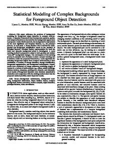
penalized smoothing spline fitted to the observations yi1 , . . . , yini . Then, functional data analysis is performed on the continuous curves fi (t) rather than on the noisy observations yi1 , . . . , yini . For ease of notation we will suppress the subscript i and write yt = f (t) for the functional object and D(m) yt = f (m) (t) for its mth derivative. Consider Figure 1 for illustration. The circles in the top panel of Figure 1 correspond to a scatterplot of bids placed in an auction versus their timing. The continuous curve in the top panel shows a smoothing spline of order m = 4 using a smoothing parameter λ = 50.
3.5 3.3
Log−Price
3.7
Current Price
0
1
2
3
4
5
6
7
5
6
7
5
6
7
Price Velocity 0.00 0.05 0.10 0.15
First Derivative of Log−Price
Day of Auction
0
1
2
3
4
0.00 0.04
Price Acceleration
−0.06
Second Derivative of Log−Price
Day of Auction
0
1
2
3
4
Day of Auction
Figure 1: Current price, price velocity (first derivative) and price acceleration (second derivative) for a selected auction. The first graph shows the actual bids together with the fitted curve. One of our modeling goals is to capture the dynamics of an auction process. While yt describes the magnitude of the current price, it does not reveal the dynamics of how fast the price is changing or moving. Attributes that we typically associate with a moving object are its velocity (or its speed) as well as its acceleration. Notice that we can compute the price velocity and price acceleration via the first and second derivatives, D(1) yt and D(2) yt , respectively. Consider again Figure 1. The middle panel corresponds to the price velocity, D(1) yt . Similarly, the bottom panel shows the price acceleration, D(2) yt . The price velocity has several interesting 7
features. It starts out at a relatively high mark which is due to the starting price that the first bid has to overcome. After the initial high speed, the price increase slows down over the next several days, reaching a value close to zero mid-way through the auction. A close-to-zero price velocity means that the price increase is extremely slow. In fact, there are no bids between the beginning of day 2 and the end of day 4 and the price velocity reflects that. This is in stark contrast to the price increase on the last day where the price velocity picks up pace and the price jumps up. The bottom panel in Figure 1 represents price acceleration. Acceleration is an important indicator of dynamics since a change in velocity is preceded by a change in acceleration. In other words, a positive acceleration today will result in an increase of velocity tomorrow. Conversely, a decrease in velocity must be preceded by a negative acceleration (or deceleration). The bottom panel in Figure 1 shows that the price acceleration is increasing over the entire auction duration. This implies that the auction is constantly experiencing forces that change its price velocity. The price acceleration is flat during the middle of the auction where no bids are placed. With every new bid, the auction experiences new forces. The magnitude of the force depends on the size of the price-increment. Smaller price-increments will result in a smaller force. On the other hand, a large number of small consecutive price-increments will result in a large force. For instance, the last 2 bids in Figure 1 arrive during the final moments of the auction. Since the increments are relatively small, the price acceleration is only moderate. A more systematic investigation of auction dynamics has been done in other places (Jank and Shmueli, 2008a; Bapna et al., 2008).
3
Dynamics of eCommerce Processes
Many eCommerce processes are governed by changing dynamics. By dynamics we mean “change” and the rate at which this change occurs. In online auctions, for instance, price increases only slowly during most of the auction duration, only to speed up rapidly towards the end (Bapna et al., 2008). In online virtual stock markets, prices of assets sometimes speed up towards the end of the trading period, while othertimes they slow down (Foutz and Jank, 2007). Dynamics capture the rate at which this change occurs. In that sense, dynamics describe the rate at which information cascades through all the levels and participants of eCommerce processes. Dynamics form an important component of our understanding of eCommerce processes. Knowledge of dynamics can lead to more accurate process predictions (Foutz and Jank, 2007; Wang et al., 2008a) and they can also lead to a better understanding of what happens “behind the scenes.” In
8
the eCommerce world, many important agent-decisions and -interactions remain unobserved. For instance in online auctions, we do not know the true strategy of bidders, we do not know how they interact with other bidders, and how they change their strategies in the face of competition. In that sense, many behavioral aspects of the auction process are unobserved. What we do observe, though, is how different bidders’ behavior results in changing auction dynamics. Thus, the ability to measure and model dynamics is a first step towards a better understanding of what drives eCommerce processes. There are many different ways of measuring and modeling dynamics. A recent stream of research (Jank and Shmueli, 2006a, 2008a,b; Bapna et al., 2008; Wang et al., 2008a,b) has focused on taking advantage of the very flexible functional data models introduced in Section 2. Functional data models are flexible because they do not impose parametric restrictions; they also allow for a unified treatment of temporal and cross-sectional data and result in a natural way of gauging process dynamics. One powerful approach borrows ideas from physics by fitting differential equation models to functional data. Wang et al. (2008b) uses a novel test for multiple comparison of functional differential equation models and finds that dynamics are quite different, even for auction processes that sell the identical item. Jank and Shmueli (2008b) develops a novel functional differential equation tree to segment dynamics based on characteristics of the auction process. Functional differential equation models are an area of research that currently receives a tremendous amount of interest (Ramsay et al., 2007). The existence of dynamics poses many challenges in eCommerce research. One of these challenges is explaining their causes. In the following, we describe a case study in the context of simultaneous auctions. We find that dynamics are partially explained by heavy bidder competition.
3.1
Case Study I: Explaining Price Dynamics in Simultaneous Online Auctions
Recent studies on online auctions have concluded that price dynamics (such as rate of change in price or price velocity) play an important role in providing insightful information about auction characteristics (Bapna et al., 2008; Reddy and Dass, 2006) and in improving prediction accuracy for price forecasts (Wang et al., 2008a). One of the questions that remains unanswered, however, is what exactly cause dynamics? In this section, we shed light on this question in the context of simultaneous online auctions (SOA) of contemporary Indian art. Particularly, we show that
9
direct inclusion of bidder competition in price forecasting models deems price dynamics information redundant. This in turn suggests that dynamics capture bidder competition in auctions. To do so, we proceed in two steps. We first illustrate the superiority of forecasting models with price dynamics, similar to the work of Wang et al. (2008a); then we show that this superiority vanishes when bidder competition is included directly into the forecaster. Many prior studies on dynamics are in the context of eBay and eBay-like online auctions. Such online auctions sell items independently of each other, meaning that beginning and ending times of auctions are not related. Recently, another auction format, namely SOA, is gaining popularity in the fine arts and collectibles market. Unlike eBay, where auctions are held for 3-7 days, SOA have a shorter duration (typically 2-3 days). They sell multiple items simultaneously in a firstprice ascending auction format. This means that auctions start and end at the same time for all the items. Since most items sold are highly complementary, bidders are frequently observed to compete against one another across one or more items. This leads to two types of dyadic bidder competition, namely within-auction competition and between-auction competition (Dass et al., 2007). In contract, bidders in eBay auctions rarely interact with each other in more than one auction at a time as they seldom have demand for similar products at the same time. Further, eBay has recently changed their policy to mask the bidders’ identities. Thus, even though some bidders may compete across multiple auctions, it is impossible for them to identify each other and thus realize between-auction competition. Further, unlike eBay auctions, SOAs have a soft closing time where the auction automatically extends in case of a late bid. This auction design not only encourages bidders to bid early (Roth and Ockenfels, 2002), but also discourages sniping in the last moments. Finally, SOAs are organized by only one seller, i.e. the auction house (similar to the Christie’s and Sotheby’s auctions), whereas eBay provides an auction platform for many different sellers. We start our investigation by developing two dynamic models (DM-I and DM-II) based on Functional Data Analysis to predict the price of an auction “in progress.” The fundamental difference between these two models is that DM-I incorporates both the price and price velocity, whereas DM-II incorporates only price. Both these models also include static pre-auction information such as auction characteristics (opening bid), item characteristics (size of the item, type of artwork), and artist characteristics (artist reputation, previous auction history). We compare the prediction accuracy with an entirely static model (ST) which is based on the above static information and
10
does not have any dynamic components. Another benchmark model is a simple dynamic model (DM-0) that includes in addition to the static information also the price at the time of prediction. We build DM-I and DM-II using the framework of Wang et al. (2008a). We first split the dataset into two parts, a training set (70% of the auctions) and validation set (30% of the auctions). The modeling approach consists of four components. The first component recovers the underlying price curve and its dynamics from the observed data. Since bids arrive at unevenly spaced time intervals, we need the flexibility of FDA to obtain the underlying price curve and its first order derivative (i.e. the rate of change in price or price-velocity). This is done by interpolating the raw data and sampling at a common set of time points to account for the irregular spacing of the bid arrivals. Then, the underlying price curves are recovered using penalized monotone curves (Ramsay and Silverman, 2005a; Simonoff, 1996). The second component fits a polynomial-trended linear regression model with autoregressive (AR) residuals to the price dynamics along with timevarying predictors. These two components are performed on the training set. The third component forecasts the price dynamics from the estimated model in the second component. Finally, in the fourth component, we forecast the actual price with DM-I and DM-II using the forecasted pricedynamics from the third component together with other time-varying and time-invariant predictors. The last two components are performed on the validation set only. Note that the training set consists of auctions that are fully observed between the start and end; in contrast, auctions in the validation set are only partially observed, i.e. information is only available until time T, the time at which a forecast is desired. T is flexible and can be set by the user. For more details, please see Wang et al. (2008a). To compare the accuracy of all forecasters, we compute their mean absolute percentage error (MAPE) on the holdout sample (left panel in Figure 2). The results show that both dynamic models, DM-I and DM-II, outperform the static model ST and the simple dynamic model DM-0. Further, in lines with prior findings, DM-I is also superior to DM-II, once again supporting the importance of price dynamics in the prediction process. (MAPE: DM-I < DM-II < DM-0 < ST) Next, we explore the cause of price dynamics. While no prior research has investigated this question in detail, some studies (Ariely and Simonson, 2003; Heyman et al., 2004) hint at the bidder rivalry as a possible answer. Based on this assertion, we quantify rivalry at the dyadic bidder level to measure within-auction and between-auction competition and incorporate them into our dynamic model to generate new DM-I and DM-II. Within-auction competition captures the rivalry-intensity
11
between two specific bidders in an auction. Operationally, it is computed as the maximum number of repeated sequential bids between two specific bidders in an auction. For every auction, we first determine the unique pairs of bidders participating in it. Then for each of these bidder pairs, we count the number of times the two bidders bid sequentially (i.e. A > B > A). The maximum number of such bids among all the bidder pair in an auction denotes the within-auction competition. Between-auction competition measures the spread of the rivalry between bidders across multiple auctions and thus, measures the competitive reach of a bidder pair across several auctions. Like the previous measure, we first determine the number of unique bidder pairs. Then, for all the bidder pairs, we count the number of auctions in which the pair is competing simultaneously. The between-auction competition for one auction is the average value across all pairs. We now incorporate these two competition components into DM-I, DM-II and again forecast price on the validation set. The right panel in Figure 2 shows the predictive performance of these new models; we can see that the difference between DM-I and DM-II has vanished. This suggests that given direct competition information, the dynamic component loses its predictive usefulness. This also suggests that bidder competition may be a major source of the dynamics. It is further noted that the dynamic models also outperform the static models in this set of analyzes. MAPE DM−0 DM−I DM−II
DM−0 DM−I DM−II
0.10
0.15
0.05
0.10 0.00
0.00
0.05
% Error
ST
0.15
ST
0.20
0.20
MAPE
0.75
0.80
0.85
0.90
0.95
1.00
0.75
Last 18 Hours of Auction
0.80
0.85
0.90
0.95
1.00
Last 18 Hours of Auction
Figure 2: Left panel: Models DM-I, DM-II, ST and DM-0 without bidder competition components; Right panel: same models with the bidder competition.
12
4
Competition between eCommerce Processes
In this section we focus on competition between eCommerce processes. An example is competition between simultaneous auctions that compete for the same bidders (in order to achieve the highest price); competition could also occur between sellers selling the same (or similar) products, or between auction platforms (e.g. eBay vs. Yahoo! auctions). Competition can also occur in other eCommerce processes. For instance, virtual stock markets (e.g. www.hsx.com) trade stock for hollywood movies. If two movies are scheduled to be released around the same time, then the amount of competition between the two movies (if any) could be reflected in the trading paths for the individual movie stocks. There are many other examples of competition between eCommerce processes. Statistically, it is hard to model competition for several reasons. First, finding a suitable measure for competition is not easy. One idea is to use the concept of correlation: the stronger the correlation between two processes, the more they compete with one another. However, it is very hard to define a statistical correlation measure for continuous processes, in part because eCommerce processes are not perfectly aligned and often only partially overlap. Online auctions are a point in case: when one auction ends, another one is about to start. Second, many processes are not perfectly identical (e.g. auctions for Microsoft Xbox gaming stations vs Sony Playstations). Dealing with varying degrees of similarity requires new statistical concepts for modeling (Jank and Shmueli, 2007) or visualizing (Hyde et al., 2006) such data. In the following, we describe a case study in the context of eBay’s online auctions. The study shows that the information from concurrent auctions matters (i.e., it matters in terms of the final price), and that by incorporating such information into a forecasting model one can achieve automated bidding systems that outperform classical bidding strategies (such as early bidding or last-moment sniping) in terms of efficiency and realized consumer surplus.
4.1
Case Study II: Competition between Online Auctions
The left panel in Figure 3 shows a calendar plot (Jank and Shmueli, 2005) of eBay auctions for a particular item (new Palm M515 handheld devices) over a certain period of time (March 14 until May 31). We can see that, at any point in time, many auctions are taking place. Since all auctions sell the identical item, bidders must decide between many competing auctions. What makes the bidder’s decision crucial for his or her bottom line is that prices vary significantly (between $170 and $280, in this case). Thus, a poor decision on the bidder’s part can lead to a large loss in 13
consumer surplus.
200 100
150
Live bid
240 220
0
160
180
50
200
Closing prices
260
250
280
300
300
Auction Calendar Plot
3/14
3/29
4/14
4/29
5/14
3/14
3/19
3/24
3/29
Calendar time
Calendar time
Figure 3: Left panel: Calendar plot of closing prices vs calendar time. Each line in the graph represents an auction, the length of the line corresponds to the length of the auction; the y-axis denotes the closing price, and the x-axis denotes calendar time. Right panel: A snapshot of the live price process of competing products during eBay auctions. The circles denote the arrival of new bids. The horizontal lines mark the time periods during which the price in an auction remains unchanged. Making informed bidding decisions in the face of auction competition is extremely hard due to information overload. Consider again Figure 3 (right panel). It shows a snapshot of the live price processes of competing auctions and it represents the information that bidders see while bidding. At any point in time, bidders see many simultaneous auctions. Each of these auctions carries different information about the auction-outcome (i.e. the final price): auctions that have only just begun carry less information about the final price compared to auctions that are almost closing. It is hard for bidders to process all of this information “manually” and to pick the auction that results in the lowest projected price. We propose a data-driven solution to this problem by modeling auction competition statistically. However, statistical models for competition are challenging for a variety of reasons. The price processes in Figure 3 form time series that are strongly misaligned and that are also of different length; modeling the information across misaligned time series of different length is not straightforward. Moreover, each price process experiences changes in price dynamics: prices usually move rather slowly during the earlier and especially middle parts of the auction, only to speed up heavily towards the auction-end. Classical time series models do not account for changes in price dynamics. And lastly, one of the modeling challenges is to incorporate competition, that is, the effect of what happens in other auctions. None of these challenges is easily handled in classical time series models.
14
1200 1000
250
400
600
price−velocity
800
200 150
live price
100
0
200
50 0
T−1
T
T+1
T−1
calendar time
T
T+1
calendar time
Figure 4: Smooth price paths (left panel) and corresponding velocities (right panel). The solid line corresponds to the focal auction; the broken line illustrate simultaneous, competing auctions. We propose an innovative approach based on functional data analysis (introduced in Section 2). In that approach, we use data smoothing to create smooth representations of the observed and noisy price processes. For an example of the resulting smooth price curves, consider the left panel of Figure 4. Notice that price curves are arranged over calendar time, thus they are extremely misaligned. In order to cope with misaligned curves and curves of different length, we evaluate each curve on a grid. Let T be the time of a desired bidding decision. Then, our approach estimates a forecasting model from the information between time T − 1 and T and uses this model to predict price at time T + 1. Moreover, since price curves are smooth, we can estimate price dynamics via their first or second derivatives. The right panel of Figure 4 shows the price velocities (i.e. first
200
250
derivatives) for the price curves in the left panel.
150
P2
100
live price
P1
P3
0
50
P4
T
calendar time
Figure 5: The solid line is the focal auction and the broken lines correspond to simultaneous, competing auctions. T corresponds to the time of decision making and p1 through p4 is the price information from all auctions available at that time.
15
One major component of our model is competition. That is, we want to capture the effect of what happens in other, simultaneous auctions. To that end, we must first define meaningful measures for competition. There are many different ways of defining competition measures and we explore several alternatives below. All measures are driven by the same general principle which is illustrated in Figure 5. We define a focal auction (indicated by the solid line in Figure 5) as the auction for which a bidder wants to decide whether or not to bid on. At time T of decision-making, there are several other auctions that take place simultaneous (indicated by the dotted lines). One meaningful measure of competition is the level of price in other auctions. In our example, there are four different prices levels at time T , varying from high (p1) to low (p4). The price level in the focal auction at that time is p3. Thus, a possible measure for the price competition is given by the average price in concurrent auctions (which we denote by c.avg.price), that is, by the average of p1, p2 and p4. In similar fashion, the average price-velocity (c.avg.vel) in concurrent auctions would be the average of the corresponding price-velocities, and so on. In this report, we investigate several different competition features and their impact on the final price of the focal auction. (For a more comprehensive investigation, see Zhang and Jank (2008).) The results are summarized in Table 1. Table 1: Competition features and their price effect. The first two columns show the name and a short explanation of the competition feature. The last column shows the effect on the final price of the focal auction. N ame c.avg.price c.avg.vel c.avg.acc c.avg.t.lef t
Explanation Average price of concurrent auctions Average price-velocity of concurrent auctions Average price-acceleration of concurrent auctions Average time left of concurrent auctions
Ef f ect positive negative negative negative
We observe several interesting effects in Table 1. First, c.avg.price has a positive effect implying that, if price is high in concurrent auctions (relative to the focal auction), then this has a positive effect on the price of the focal auction. In other words, high price levels in other, competing auctions will make bidders search for different auctions (with a lower price) and subsequently drive up the price in those auctions. The effects of the concurrent dynamics (c.avg.vel and c.avg.acc) are negative. This may indicate information cascading or herding: if the “buzz” for other auctions increases, then this will hurt the price of the focal auction. Similarly, the time that is left in other auctions (c.avg.t.lef t) negatively influences price in the focal auction, since bidders have more time
16
to make informed decisions outside of the focal auction. Using the competition features from Table 1 (together with additional information such as the auction format, information about the seller, the bidders and the price dynamics), we build a forecasting model for price in competing auctions. Then, in the next step, we build a comprehensive bidding strategy around our forecasting model. The idea is based on maximizing consumer surplus, which refers to the difference between the bidders’ willingness to pay and the price actually paid. We formulate an automated algorithm for selecting the optimal auction to bid on, and for determining the optimal bid-time and -amount. The optimal auction provides bidders with the highest surplus, and the optimal bid-amount equals the predicted closing price. This strategy automates the entire decision-making process, and, in contrast to early or late bidding strategies, it frees the bidder of time-constraints since bidding can occur immediately. (For more details see Zhang and Jank (2008).) We conduct a simulation study to compare our automated bidding strategy to alternate bidding approaches such as early bidding (Bapna et al., 2004) or last-moment sniping (Roth and Ockenfels, 2002). Early bidding is often used as a signal for the bidder’s commitment and intends to deter other bidders. Last-moment sniping is a popular strategy because it does not allow enough time for other bidders to react. In our simulation, we assume that bidders’ willingness-to-pay (WTP) are drawn from a uniform distribution that is symmetrically distributed around the market value. A bidder randomly draws from this distribution and then bids according to one of three strategies: Under early bidding, the bidder bids his WTP at the end of the first day of the auction1 . Under last-moment sniping the bidder waits until the last minute of the auction and then bids 1% over the current price. And finally, under our automated bidding strategy, the bidder bids the price predicted by our forecasting model. Note that in contrast to early bidding or last-moment sniping, the bidding decision in our strategy is free of time, i.e. the bidder bids immediately without having to wait for the end of the first auction-day or for the last minute of the auction. While this advantage may not mean much to bidders who use automated bidding agents such as www.cniper.com, not all eBay bidders use this technology. Moreover, such technology is only available for the eBay market and not for smaller, more specialized auction markets (such as those for Indian art mentioned on Section 3). We also want to point out that our simulations are set up such that, under each strategy, bidders will only bid if the current auction price is less than their WTP; otherwise, the bidder will 1
Note that most eBay auctions are between 3 and 10 days long.
17
move on to another auction, and so on. Table 2: The table shows the result of 3 different bidding strategies: sniping, early bidding and automated bidding according to the data-driven forecasting model. The second column shows the probability of wining an auction; the third column shows the resulting consumer surplus. Bidding Rule Sniping Early Bidding Automated Bidding
Prob(Win) .92 .62 .61
Avg(Surplus) $18 $0 $32
The results are presented in Table 2. We find that, although snipers have the highest probability of winning, our automated and data-driven strategy results in a much higher surplus. It also results in considerably less time devoted to the process of bidding since no manual monitoring of the auction process is necessary. Moreover, early bidders have the lowest average winning probability and surplus. We also investigate the impact of the prediction window on the resulting surplus, and find that, as the width of the window increases, consumer surplus increases while the probability of winning decreases.
5
User Networks in eCommerce
Another challenge of eCommerce data is the existence of networks created by its users. For instance, customers that (repeatedly) buy from the same seller form a network with that seller. Bidders who intentionally bid on the same auction as other bidders (see, e.g., www.auctionshadow.com) form a different type of network with one another. More generally, users that visit each other’s websites, post on each other’s blogs, or “meet” online in one way or the other are all linked in a network. While this data challenge is intrinsically related to the previous challenge of competition, we discuss it separately, partly due to the spacial nature of networked data. Modeling user networks is complicated by the fact that data arrive in the form of ties and nodes, rather than in the more classical form of vectors and matrices. This new data structure motivates the need for new methods of analysis which has given rise to the new field of network analysis, and in particular social network analysis (SNA) (e.g. Scott, 2000). Social network analysis views social relationships in terms of ties and nodes. Nodes are the individual actors within the networks, and ties are the relationships between the actors. In its simplest form, a social network is a map of all of the relevant ties between the nodes being studied. The network can also be used to determine the
18
social capital of individual actors. These concepts are often displayed in a social network diagram (e.g. Figure 6), where nodes are the points and ties are the lines. The analysis of social networks has several objectives. On the one hand, one wants to study global aspects of the entire network such as its Betweenness, Closeness and the degree of Centrality. All of these measures quantify the connectivity of an individual to other individuals in the network. Centrality measures the number of incoming and outgoing interactions in a directed network (or the total interactions in the undirected case). There are two interpretation of this number. Freeman (1979) suggests that individuals who have many ties to other individuals are more influential and thus less dependent on other individuals. Bonacich (1987) suggests that two entities with the same centrality are not necessarily equally important. Instead, he suggests that, in addition, one needs to account for the centrality of its neighbors. The idea is that an individual that is connected to other individuals with few connections is more influential, as it makes these individuals more depended upon himself. Bonachich’s approach is commonly referred to as The Bonachich Power and is widely used in SNA literature. The closeness of an individual measures the geodesic distances to other individuals within the same graph (Sabidussi, 1966). The level of closeness of an individual is measured by the mean distance to all other individuals. A variation of closeness is called eigenvector centrality which accounts for the scores of the connected entities, as well as their geodesic distances. Hence, connections to high-scoring individuals result in a higher score for a particular individual. Betweenness is another measure of the network and measures individuals that are connected on shorter paths than others. In other words, individuals with a low betweeness score have a faster reach of other network members (Freeman, 1979). Besides global aspects of the network, one is also interested in studying local aspects, such as the existence and structural form of sub-graphs (Lubbers and Snijders, 2007). Moreover, recent research has also paid particular attention to longitudinal and dynamic aspects of networks (Snijders, 2001). User networks are important because they facilitate the flow of information between all network members. Hill et al. (2006) study the effect of networks on viral marketing and find that “networkneighbors” (i.e. those consumers linked to a prior customer) adopt a new product at a significantly higher rate. Watts and Dodds (2007) study the role of centrality of a network participant on product diffusion. The authors simulate diffusion models and find that central participants are modestly more important than average participants in product diffusion. Interestingly, the authors 19
also show that most social change is driven not by central network members, but by the easily influenced individuals who influence other easily influenced individuals. Similar applications of SNA in diffusion and promotion models are offered by Mayzlin (2002); Valente (1996) and others. An early application of SNA to online markets can be found in Dass and Reddy (2007) who study bidder interactions in simultaneous auctions. The authors address the question of existence of “key” bidders that are more influential than others on the auction outcome. They formalize the interactions as a network where nodes correspond to bidders and an arc between two bidders corresponds to competition in an auction. In the following case study, we investigate the existence and importance of user networks in online transactions. In particular, we investigate the impact of user networks on the outcome of an online auction. To that end, we derive a new measure of e-loyalty based on a combination of social network analysis and functional data models. Our preliminary analyses show that networks vary across product types and result in different types of bidder loyalty.
5.1
Case Study III: User Networks in Online Auctions and e-Loyalty
eBay is one of the largest C2C online marketplace and it enables trading between individuals and small businesses. Each day, several million items are up for sale and offered to several million potential buyers. While much of the literature up to date considers events within one auction as independent of other auctions, in reality many auctions are inter-linked. Bidders can participate in more than one auction at a time, they can purchase exclusively from one seller or from multiple sellers over time, and they can also choose among many competing products that are offered simultaneously. One result of this complex web of interactions is a seller-bidder network. In what follows, we study the effect of this network on the loyalty of bidders. One of the main challenges in understanding seller-bidder interactions is to define a suitable measure that captures the different forms of e-loyalty. The goal is to map bidders’ loyalty from an observed network to a continuous measure that ranges between multiple purchases from a single seller (high loyalty), and single purchases from multiple sellers (low loyalty). Using an innovative combination of social network analysis and functional data analysis, we we define a unique measurement for both bidders’ loyalty and sellers’ perceived loyalty. We start by defining user networks in online auctions, then define a measure of e-loyalty, and finally study the effect of loyalty on the outcome of an auction.
20
Figure 6: E-Loyalty Network for golf ball auctions. The large pink nodes correspond to sellers; the small blue nodes correspond to bidders. An arc represents an interaction between the two. 5.1.1
User Network Definition
We define a user network as the bi-partite graph in which one set of nodes represents sellers (the large pink nodes in Figure 6), the other set represents bidders (small blue nodes), and an arc between a bidder and a seller indicates that there is an interaction (a bid, in this case) between the two. The weight of the arc corresponds to the number of interactions in distinct auctions. Figure 6 shows the network of bidders and sellers for Titleist golf balls auctions that took place between August 9th, 2007 and October 2nd, 2007 on eBay. 5.1.2
A Novel Measure of E-Loyalty
One of the main challenges in understanding seller-bidder interactions is defining a suitable measure that captures the different forms of e-loyalty. Our goal is to map a bidder’s loyalty to a continuous scale that ranges between multiple purchases from a single seller (i.e. high loyalty), to many single purchases from different sellers (i.e. low loyalty). To that end, we first derive the distribution of loyalty from the seller-bidder network. We then characterize each distribution by a single score using functional principal components analysis.
21
1
1 1
1 1
1
1 1 1
1
2
4
4 10
Figure 7: Illustration: Observed seller-bidder network between bidders A,B and C, and sellers 1-10. A
B
C
Figure 8: Illustration: The top panel shows the observed loyalty distribution for each bidder from Figure 7; the bottom panel shows a smooth representation of the standardized distribution using smoothing splines. For illustration, consider the three bidders in Figure 7 (labeled “A”, “B” and “C”). Each bidder has a total of 10 interactions with different sellers. Bidder A interacts 10 times with the same seller, thus his loyalty is very high and exclusive to that seller. Bidder B interacts 4 times each with sellers # 1 and #2, respectively, and 2 times with seller #3. We can consider bidder B’s loyalty as moderate. In contrast, bidder C has a single interaction with each of 10 sellers. Bidder C is the least loyal of all three bidders. We can summarize each bidder’s loyalty by their corresponding loyalty distributions. Figure 8 shows the observed loyalty distributions (i.e. histograms, top panels) and their corresponding 22
smooth representations (bottom panels). Smooth representations eliminate noise; they also allow for a very flexible and granular way of capturing and comparing different forms of loyalty distribution. We can see that very loyal bidders (i.e. such as bidder A) distribute all their loyalty to a single seller; thus their loyalty distribution is very steep and shows only little variance. In contrast, bidders with little loyalty (e.g. bidder C) display distributions that are very flat and highly variable. The next step is to summarize each distribution by a single number that captures similarities (and differences) across different loyalty distributions. This can be done via functional principal components analysis (fPCA), a functional version of principal components analysis (see Ramsay and Silverman, 2005b). Functional principal components analysis is similar in nature to ordinary PCA; however, rather than operating on data-vectors, it operates on functional objects (continuous curves, in our context). To make the discussion more concrete, let us assume that loyalty curves are measured at t discrete time points. Let Y s = (y1s , . . . , yns ) denote the (n × t) matrix consisting of all smooth loyalty curves. Let R := Corr(Y s ) be the n × n correlation matrix obtained from Y s . Analogous to ordinary principal components analysis, R is decomposed into PT ΛP, where Λ is the n × n matrix of eigenvalues and P = [e1 , e2 , . . . , en ]T is the n × t corresponding matrix of eigenvectors. In this simplified example, each ei , i = 1, . . . , n is a (t × 1) vector, but in reality ei is a continuous function in time, i.e. ei = ei (t). We can think of each eigenvector ei as a loyalty-defining characteristic. Each eigenvector ei , i = 1, . . . , n captures λi × 100% of the variability in Y s , where λi is the ith eigenvalue or the i-th diagonal element in Λ. The eigenvector corresponding to the largest eigenvalue is denoted as the first principal component (PC hereafter). Similarly, the second PC is the eigenvector that corresponds to the second highest eigenvalue, and so on. Common practice is to choose only those eigenvectors that correspond to the largest eigenvalues, i.e. those that explain most of the variation in Y s . By discarding those eigenvectors that explain no or only a very small proportion of the variation, we capture the most important characteristics of the observed data patterns without much loss of information. In our context, the first eigenvector captures 93% of the variation, so we summarize loyalty by the first eigenvector of the smooth loyalty curve. To better understand the derived loyalty measures, we first conduct a small simulation study. We simulate a network of 150 bidders interacting with 50 sellers. We assume that bidders’ loyalties follow a log-normal distribution LogNormal(µ, σ) with a fixed location parameter µ 2
2
and a shape
The actual value of the location parameter does not have an effect on our simulation since we normalize the simulated data. By normalizing, we also do not differentiate between bidders that have the same level of loyalty but
23
V=5
V=3
V=1
Figure 9: Simulated e-Loyalty: Larger values of σ correspond to higher levels of loyalty to the same seller. parameter σ that varies between 1 and 5. Figure 9 illustrates the simulations. A small value of σ (e.g. σ =1) corresponds to a very low loyalty, whereas bidders with high loyalty to the same seller experience higher values of σ. In our simulations, we consider four different types of networks. In the first network, loyalty of all bidders is randomly distributed between not loyal (σ = 1) and very loyal (σ = 5). In the second and third network, all bidders are either completely loyal (σ = 5) or completely unloyal (σ = 1), respectively. Finally, in the forth network we consider a mixture of two different segments of bidders: some that are loyal and others that are unloyal bidders. Figure 10 shows the results. The second panel displays the observed bidder loyalty distributions; the third panel displays the associated first functional principal component score (fPCS). The first fPCS captures the strength of loyalty: bidders that are extremely loyal have a very steep loyalty distribution (second row in Figure 10); hence their fPCS score is high. Similarly, unloyal bidders (third row in Figure 10) have a very low fPCS score. We can see that the fPCS score efficiently captures differences in a bidder’s loyalty distribution in one single number and characterizes loyal and unloyal bidders on a continuous scale. different number of interactions.
24
Loyalty Distributions
First PC Score
40 0
0.0
10
0.2
20
30
Frequency
0.6 0.4
probability
50
0.8
60
70
1.0
Network
0
2
4
6
8
10
−1.0
−0.5
seller
0.5
1.0
0.5
1.0
0.5
1.0
0.5
1.0
40 0
0.0
10
0.2
20
30
Frequency
0.6 0.4
probability
50
0.8
60
70
1.0
Random
0.0 Score
0
2
4
6
8
10
−1.0
−0.5
seller
40 0
0.0
10
0.2
20
30
Frequency
0.6 0.4
probability
50
0.8
60
70
1.0
All Loyal
0.0 Score
0
2
4
6
8
10
−1.0
−0.5
seller
40 0
0.0
10
0.2
20
30
Frequency
0.6 0.4
probability
50
0.8
60
70
1.0
All Non-Loyal
0.0 Score
0
Two Segments
2
4
6
8
seller
10
−1.0
−0.5
0.0 Score
Figure 10: Simulated Loyalty: The middle column shows the observed bidder loyalty distributions; the right column shows the first functional principal components score.
25
5.1.3
Network Comparison
We apply our loyalty measures to two different markets for roller-ball pens: auctions for Parker pens and Cross pens, collected from eBay on Dec-2007. Both are of similar value (around $30), with the Parker pen being slightly more expensive. Figure 11 shows the overlapping networks for both products. Bidders are denoted by white, square nodes; sellers are denoted by triangles. Black triangles denote sellers that sell both Parker and Cross pens; red and green triangles denote sellers that sell a single brand (either Parker (red) or Cross (green) pens). The arcs are dyed similarly: black arcs represent interactions across both networks, while red (green) arcs denote interactions exclusively in the Parker (Cross) network. We can see that the loyalty networks are rather complex. Some bidders bid on only one brand (Parker or Cross), while others bid on both. For those bidders who bid on both brands, they can choose to interact with only one seller (who sells both brands), or with many different sellers. We can see that some bidders are always loyal to the same seller, regardless of the brand (i.e. across both networks), while others are loyal to one seller for one brand, but loyal to a different seller for the other brand. Yet, other bidders display only little loyalty and interact with a multitude of sellers. We investigate these initial observations in more detail below. Figure 12 compares the two product-networks. We can see that there is a significantly larger amount of Cross auctions compared to Parker auctions (4041 vs. 2501), and, as a result, a larger number of bidders and sellers in the Cross network. Most bidders participate in 1 or 2 auctions (row #5 in Figure 12), but this number is a bit more right-skewed for the Cross auctions. Similarly, most sellers have between 2 and 4 auctions (row #6) with a somewhat higher skew again in the Cross network. Row #7 displays the resulting loyalty curves for each bidder and row #8 shows the corresponding loyalty scores based on the first fPCA. We can see that most bidders show strong loyalty (cf. steep loyalty curves in row #7 or high loyalty scores in row #8). However, it is interesting to note that the Cross network shows a stronger left-skew in the loyalty distribution, suggesting a larger proportion of non-loyal bidders for this product. We are quick to caution though that the (numerical) difference may merely be the result of the larger number of auctions and bidders for this product. While the above network differences may be entirely due to the different network sizes, we obtain a more careful picture by comparing the loyalty of individual bidders across the two productnetworks. Figure 13 shows the loyalty curves for bidders who participate at least 3 times in both the 26
Loyal to the same seller in both networks
Loyal in one network
Always loyal
Loyal to a mutual seller in one network only Figure 11: e-Loyalty networks for Parker and Cross pens. Sellers are denoted by triangles, bidders by squares; arcs denote an interaction between the two. Red (green) arcs denote bidder-seller interactions exclusively for Parker (Cross) pens, black arcs denote an interaction between a bidder and a seller for both brands. Parker as well as the Cross network (total of 9 bidders). The solid lines in Figure 13 correspond to their corresponding loyalty in the Cross network, while the dashed lines correspond to the Parkerloyalty. We can see that while some bidders (e.g. elvis 2080; mikeresnick) display equal loyalty (high or low) in both networks, others (e.g. scr8899) are extremely loyal in the Parker network, but non-loyal for the other product.
6
Conclusion
This paper focuses on how novel statistical method and thought can be used to take advantage of the rich data found in online markets. Such data tend to have non-standard structure in the sense that over-the-shelf statistical methodology is often not adequate, neither for capturing the
27
Measure #Sellers #Bidders #Auctions Distribution of auctions per bidder
Parker 241 1101 2501
Cross 585 2354 4041
Distribution of auctions per seller
Loyalty curves
Loyalty distribution
Figure 12: Comparison of brand-networks: the left panel shows loyalty summaries for the Parker network; the right panel show the corresponding summaries for the Cross network. entire information in the data, nor for answering new research questions based on the data. Three particularly challenging aspects of eCommerce data are dynamics, competition, and user networks. All three phenomena arise from the interaction between users, between processes, and between markets. Marked by different behavioral, economic and social forces that are often are pulling into opposite directions, the online environment is becoming increasingly interactive, networked and customized. These forces, together with their effect on the resulting transaction outcome, are now
28
Figure 13: Comparison of bidders’ loyalty curves in different product-networks. The solid lines correspond to loyalty in the Cross network, the dashed lines correspond to the Parker-loyalty. observable and measurable and as a result eCommerce data are richer in the different, often diverse pieces of information they contain. A main facet of this richness is the combination of several types of traditional data elements and the resulting new dependence structures that it brings about. Examples are combinations of cross sectional and temporal data that are extremely common in eCommerce datasets; network data and their evolution over time; competition between users for a given good or even across markets, and more. This paper illustrates that empirical research in eCommerce, though growing fast, involves many new statistical challenges. We regard these challenges as opportunities in that they call for the development of new statistical tools or the adaptation of existing statistical machinery. New ideas are needed for data representation, summarization, visualization, and modeling. Our case studies exemplify the many different challenges that arise in the context of online auctions
29
and we present some solutions and new research directions, many of which also apply to other eCommerce applications. We conclude on the note that statistics in eCommerce becomes more and more important to researchers and practitioners alike as exemplified by a recent special issue on the topic (Jank and Shmueli, 2006b), and edited book (Jank and Shmueli, 2008c), or an annual workshop series that has steadily been growing out of its inaugural event in 2005 (www.smith.umd.edu/dit/statschallenges).
References Agarwal, D. (2008). Statistical Methods in eCommerce Research, chapter Statistical Challenges in Internet Advertising, page forthcoming. Wiley and Sons. Ariely, D. and Simonson, I. (2003). Buying, bidding, playing, or competing? value assessment and decision dynamics in online auctions. Journal of Consumer Psychology, 13(1 & 2):113–123. Journal of Consumer Psychology. Bapna, R., Goes, P., Gopal, R., and Marsden, J. R. (2006). Moving from data-constrained to dataenabled research: Experiences and challenges in collecting, validating and analyzing large-scale e-commerce data. Statistical Science, 21 (2):116–130. Bapna, R., Goes, P., Gupta, A., and Jin, Y. (2004). User heterogeneity and its impact on electronic auction market design: An empirical exploration. MIS Quarterly, 28:1:21–43. Bapna, R., Jank, W., and Shmueli, G. (2008). Price formation and its dynamics in online auctions. Decision Support Systems, 44:641–656. Bapna, R., Jank, W., and Shmueli, G. (2008 (in press)). Consumer surplus in online auctions. Information Systems Research. Bonacich, P. (1987). Power and Centrality: A Family of Measures. The American Journal of Sociology, 92(5):1170–1182. Borle, S., Boatwright, P., and Kadane, J. B. (2006). The timing of bid placement and extent of multiple bidding: An empirical investigation using ebay online auctions. Statistical Science, 21 (2):194–205. Dass, M. and Reddy, S. K. (2007). Bidder networks and price dynamics in online auctions. Working paper. 30
Dass, M. and Reddy, S. K. (2008). Statistical Methods in eCommerce Research, chapter An Analysis of Price Dynamics, Bidder Networks and Market Structure in Online Auctions, page forthcoming. Wiley and Sons. Dass, M., Reddy, S. K., and Du, R. (2007). Dyadic bidder interactions and key bidders in simultaneous online auctions. Fienberg, S. E. (2006). Privacy and confidentiality in an e-commerce world: Data mining, data warehousing, matching and disclosure limitation. Statistical Science, 21 (2):143–154. Forman, C. and Goldfarb, A. (2008). Statistical Methods in eCommerce Research, chapter How has electronic commerce research advanced understanding of the offline world?, page forthcoming. Wiley and Sons. Forsythe, R., Rietz, T. A., and Ross, T. W. (1999). Wishes, expectations, and actions: A survey on price formation in election stock markets. Journal of Economic Behavior & Organization, 39:83–110. Foutz, N. and Jank, W. (2007). The wisdom of crowds: Pre-release forecasting via functional shape analysis of the online virtual stock market. Marketing Science Institute Report, 07–114. Freeman, L. (1979). Centrality in social networks: Conceptual clarification. Social Networks, 1(3):215–239. Ghose, A. (2008). Statistical Methods in eCommerce Research, chapter The Economic Impact of User-Generated and Firm-Published Online Content: Directions for Advancing the Frontiers in Electronic Commerce Research, page forthcoming. Wiley and Sons. Ghose, A. and Sundararajan, A. (2006). Evaluating pricing strategy using e-commerce data: Evidence and estimation challenges. Statistical Science, 21 (2):131–142. Haruvy, E., Popkowski Leszczyc, P., Carare, O., Cox, J., Greenleaf, E., Jank, W., Jap, S., Park, Y.-H., and Rothkopf, M. (2008). Competition between auctions. Marketing Letters, forthcoming. Heyman, J. E., Orhun, Y., and Ariely, D. (2004). Auction fever: The effect of opponents and quasi-endowment on product valuations. Journal of Interactive Marketing, 18(4):8–21. Hill, S., Provost, F., and Volinsky, C. (2006). Network-based marketing: Identifying likely adopters via consumer networks. Statistical Science, 22 (2):256–276. 31
Hyde, V., Jank, W., and Shmueli, G. (2006). Investigating concurrency in online auctions through visualization. The American Statistician, 60:241–250. Hyde, V., Jank, W., and Shmueli, G. (2008). Statistical Methods in eCommerce Research, chapter A Family of Growth Models for Representing the Price Process in Online Auctions, page forthcoming. Wiley and Sons. Jank, W. and Shmueli, G. (2005). Visualizing online auctions. Journal of Computational and Graphical Statistics, 14(2):299–319. Jank, W. and Shmueli, G. (2006a). Functional data analysis in electronic commerce research. Statistical Science, 21 (2):155–166. Jank, W. and Shmueli, G. (2006b). Statistical Challenges in Electronic Commerce Research. Statistical Science, 21. Jank, W. and Shmueli, G. (2007). Modeling concurrency of events in online auctions via spatiotemporal semiparametric models. Journal of the Royal Statistical Society - Series C, 56:1–27. Jank, W. and Shmueli, G. (2008a). Handbook of Information Systems Series: Business Computing, chapter Studying Heterogeneity of Price Evolution in eBay Auctions via Functional Clustering. Elsevier. Forthcoming. Jank, W. and Shmueli, G. (2008b). Statistical Methods in eCommerce Research, chapter Modeling Price Dynamics in Online Auctions via Regression Trees. Wiley & Sons. Forthcoming. Jank, W. and Shmueli, G., editors (2008c). Statistical Methods in eCommerce Research. Wiley & Sons. Kauffman, R. J. and Wood, C. A. (2005). The effects of shilling on final bid prices in online auctions. Electronic Commerce Research and Applications, 4 (2):21–34. Lubbers, M. and Snijders, T. (2007). A comparison of various approaches to the exponential random graph model: A reanalysis of 102 student networks in school classes. Social Networks, 29 (4):489–507. Lucking-Reiley, D. (1999). Using filed experiements to test equivalence between auction formats: Magic on the internet. American Economic Review, 89(5):1063–1080.
32
Matas, A. and Schamroth, Y. (2008). Statistical Methods in eCommerce Research, chapter Optimization of Search Engine Marketing bidding strategies using statistical techniques, page forthcoming. Wiley and Sons. Mayzlin, D. (2002). The Influence OF Social Networks ON The Effectiveness OF Promotional Strategies. Yale School of Management Working Paper. Park, Y.-H. and Bradlow, E. (2005). An integrated model for whether, who, when, and how much in internet auctions. SSRN eLibrary. Pennock, D. M., Lawrence, S., Giles, C. L., and Nielsen, F. A. (2001). The real power of artificial markets. Science, 291(5506):987–988. Ramsay, J., Hooker, G., Campbell, D., and Cao, J. (2007). Parameter estimation for differential equations: A generalized smoothing approach. Journal of the Royal Statistical Society - Series B, 69 (5):741–796. Ramsay, J. and Silverman, B. (2005a). Functional Data Analysis. Springer Series in Statistics. Springer-Verlag, New York, 2nd edition. Ramsay, J. and Silverman, B. (2005b). Functional Data Analysis. Springer. Reddy, S. K. and Dass, M. (2006). Modeling online art auction dynamics using functional data analysis. Statistical Science, 21(2):179–193. Roth, A. E. and Ockenfels, A. (2002). Last-minute bidding and the rules for ending second-price auctions: Evidence from ebay and amazon auctions on the internet. The American Economic Review, 92(4):1093–1103. Sabidussi, G. (1966). The centrality index of a graph. Psychometrika, 31(4):581–603. Scott, J. (2000). Social Network Analysis: A Handbook. Sage Publications Inc. Shmueli, G., Russo, R. P., and Jank, W. (2007). The barista: A model for bid arrivals in online auctions. Annals of Applied Statistics, 1 (2):412–441. Simonoff, J. (1996). Smoothing Methods in Statistics. Springer-Verlag, New York, 1st edition. Snijders, T. (2001). Sociological Methodology, chapter The Statistical Evaluation of Social Network Dynamics. Boston and London: Basil Blackwell. 33
Spann, M. and Skiera, B. (2003). Internet-based virtual stock markets for business forecasting. Management Science, 49(10):1310–1326. Stewart, K., Darcy, D., and Daniel, S. (2006). Opportunities and challenges applying functional data analysis to the study of open source software evolution. Statistical Science, 21 (2):167–178. Telang, R. and Smith, M. D. (2008). Internet exchanges for used digital goods. SSRN eLibrary. Valente, T. (1996). Network models of the diffusion of innovations. Computational & Mathematical Organization Theory, 2(2):163–164. Wang, S., Jank, W., and Shmueli, G. (2008a). Explaining and forecasting online auction prices and their dynamics using functional data analysis. Journal of Business and Economic Statistics, to appear. Wang, S., Jank, W., Shmueli, G., and Smith, P. (2008b). Modeling price dynamics in ebay auctions using principal differential analysis. Journal of the American Statistical Association, to appear. Watts, D. J. and Dodds, P. S. (2007). Influentials, networks, and public opinion formation. Journal of Consumer Research, in press. Yao, S. and Mela, C. F. (2007). Online auction demand. SSRN eLibrary. Zhang, S. and Jank, W. (2008). An automated and data-driven bidding strategy for online auctions. Technical report, RH Smith School of Business, University of Marylnad.
34