Modeling the Dynamics of Long-Term Variability of ... - CiteSeerX

VOLUME 4

JOURNAL OF HYDROMETEOROLOGY

JUNE 2003

Modeling the Dynamics of Long-Term Variability of Hydroclimatic Processes OLI G. B. SVEINSSON

AND JOSE

D. SALAS

Department of Civil Engineering, Colorado State University, Fort Collins, Colorado

DUANE C. BOES Department of Statistics, Colorado State University, Fort Collins, Colorado

ROGER A. PIELKE SR. Department of Atmospheric Science, and Colorado Climate Center, Colorado State University, Fort Collins, Colorado (Manuscript received 26 December 2001, in final form 9 September 2002) ABSTRACT The stochastic analysis, modeling, and simulation of climatic and hydrologic processes such as precipitation, streamflow, and sea surface temperature have usually been based on assumed stationarity or randomness of the process under consideration. However, empirical evidence of many hydroclimatic data shows temporal variability involving trends, oscillatory behavior, and sudden shifts. While many studies have been made for detecting and testing the statistical significance of these special characteristics, the probabilistic framework for modeling the temporal dynamics of such processes appears to be lacking. In this paper a family of stochastic models that can be used to capture the dynamics of abrupt shifts in hydroclimatic time series is proposed. The applicability of such ‘‘shifting mean models’’ are illustrated by using time series data of annual Pacific decadal oscillation (PDO) indices and annual streamflows of the Niger River.

1. Introduction On the annual timescale, the analysis of climatic and hydrologic processes is generally based on assumed stationarity under a time series framework or randomness under a probabilistic framework. While this assumption may be reasonable within a short time frame (a few decades depending on the particular case), empirical evidence shows that most hydroclimatic processes deviate from stationarity in the long term. To some extent the assumption of stationarity has persisted because most historical records have been too short to accurately detect nonstationarity, and because of lack of mathematical frameworks for analyzing and modeling the dynamics of nonstationary processes. However, as record lengths have increased, trends, oscillatory behavior, and sudden shifts have been observed in sample records. The main objective of this paper is to model hydroclimatic processes that shift abruptly from one stationary state into another. It appears that the first concept behind modeling sudden shifts in hydrologic time series was advanced by Hurst (1957). Subsequently Klemes (1974) and Potter (1976) further argued about the useCorresponding author address: Jose D. Salas, Department of Civil Engineering, Colorado State University, Fort Collins, CO 80523. E-mail: [email protected]

q 2003 American Meteorological Society

fulness of algorithms to model shifting behavior. Boes and Salas (1978) developed some special cases of shifting mean models and Salas and Boes (1980) further discussed their conceptual justification and their applicability to hydrology. In this paper, we expand on the earlier concepts and models and develop more versatile models that can be useful for simulating the dynamics of hydroclimatic processes exhibiting abrupt shifts. The methods suggested here are intended for simulation and generation of long sample records, rather than forecasting. Shifts in hydrologic processes may be related to climate changes (Matalas 1997). Different indices, such as oscillation indices that measure pressure or temperature differences between two locations, or solar indices that measure sunspot activity, are sometimes used to reflect climatic fluctuations. These indices often appear to change quasi-periodically with time, or shift from one random stationary state to another. Taylor (1999) investigated ice cores from Greenland glaciers to get information about climate and climate changes in the past. He concluded, that climate changes large enough to cause significant impacts on society have occurred in the past over a duration less than 10 yr. His ice core measurements also indicated that 11 700 yr ago, when the climate in the North Atlantic shifted from a dry and

489

490

JOURNAL OF HYDROMETEOROLOGY

cold ice age to a wetter and warmer climate, most of the shift occurred during a period of only 40 yr. Kite (1989) investigated changes in lake levels and streamflow sequences. He used time series analysis and spectral analysis to detect linear trends, jumps, periodicities, and other components in the hydrologic sequences. He concluded that any such detected statistical components were not the result of a climate change induced by the so-called greenhouse effect but rather the result of other natural processes. Likewise, Chiew and McMahon (1993) concluded that there was no clear evidence to suggest that trends or change in mean flow volumes of Australian rivers were caused by climate changes. They also commented that their results might be affected by short sample records with high interannual variability. Angel and Huff (1997) investigated changes in large storm rainfall in the midwestern United States. Their results showed that stations in the entire Midwest are likely to have experienced their heaviest rainfall in the recent years. Others have tried to use oscillation indices such as the Southern Oscillation (SO) often related to El Nin˜o or La Nin˜a depending on its phase, or the Pacific decadal oscillation (PDO) to explain observed variability in historical sample series. For example, Waylen and Caviedes (1986) used a three-component mixed Gumbel distribution to fit the annual maximum floods on the north Peruvian littoral. The annual maximum flood series were looked at as being produced by three different mechanisms corresponding to different ocean–atmosphere conditions: El Nin˜o, near average, and La Nin˜a. Eltahir (1996) correlated the annual Nile River flows with El Nin˜o–Southern Oscillation (ENSO), which is based on sea surface temperature. His results suggested that 25% of the variance of the annual Nile River flows was associated with ENSO. Hamlet and Lettenmaier (1999) forecasted Columbia River flows based on a given forecast of ENSO and the phase of PDO. Their results suggested that including such atmosphere–ocean information into streamflow forecasting models could result in an increase in forecast lead time of about six months. There is empirical evidence that interdecadal variability with abrupt changes in oceanic–atmospheric processes and hydrologic processes have occurred in many parts of the globe. An abrupt change, marked by a southward shift and intensification of the Aleutian low, a drop in the SST of the central North Pacific, and an increase of SST along the west coast of North America, occurred around 1976 (Trenberth 1990). Also Landsea et al. (1999) reported abrupt changes of the annual rainfall in the Sahelian region in Africa, and Thyer and Kuczera (2000) showed the long-term variability of annual rainfall in some places in Australia where several periods persistently below the long-term mean occurred. Likewise, abrupt changes have been reported in the annual streamflows of the Nile River in Africa and the Colorado River in the United States (Yevjevich 1972), the Niger River in Africa (Chung and Salas 2000), the lake levels

VOLUME 4

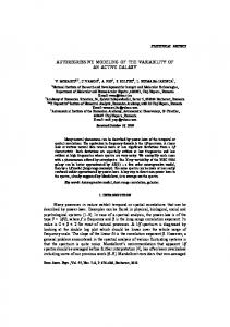
and outflows of the equatorial lakes in Africa (Salas et al. 1981), and the annual net basin supplies for Lakes Ontario and Erie in North America (Rassam et al. 1992). In addition, the recent study by Yonetani and Gordon (2001) documenting the occurrence of abrupt shifts in oceanic–atmospheric factors, such as surface air temperature and sea level pressure, resulting from a coupled atmosphere–ocean general circulation model is yet another example of why certain hydrological processes, such as rainfall and streamflow in some parts of the world, also exhibit abrupt changes. These examples also suggest the need for further analyzing and modeling hydroclimatic processes exhibiting sudden shifting behavior. Modeling the dynamics of such types of processes by using stochastic methods is the main subject of this paper. 2. Some examples of hydroclimatic time series exhibiting sudden shifts There are many examples of time series of hydroclimatic processes that show evidence of sudden shifts in one or more of their statistical properties. For instance, Mantua et al. (1997), Niebauer (1998), and Hamlet and Lettenmaier (1999) analyzed the time series of annual averages of the PDO index based on sea surface temperature. Their results suggest that several shifts have occurred since 1900. The latest such shift is suggested to have occurred around 1977. Mantua et al. (1997) defined the PDO to be in a cold phase during 1900–24 and 1947–76, and in a warm phase during the periods 1925–46 and 1977–96. Hamlet and Lettenmaier (1999) argued that based on the Columbia River flows the phase of the PDO might have shifted again in 1996 or 1997. Figures 1a,b show an update of the annual averages of the PDO index from Mantua et al. (1997). The data were downloaded from ftp://ftp.atmos.washington.edu/ mantua/pnwpimpacts/INDICES/PDO.latest. In Fig. 1a the index time series is shown along with averages of dominant phases as suggested by Mantua et al. (1997). In Fig. 1b the index series is shown with alternative choices of phases. The models proposed in this paper are intended for time series that show similar sudden shifting structure as in Fig. 1. Niebauer (1998) argued that before the regime shift in 1977, El Nin˜o and La Nin˜a conditions were about even, but after the regime shift El Nin˜o conditions were about 3 times more prevalent, due to a change of location of the Aleutian low. Gray et al. (2000) use sea surface temperature (SST) in the North Atlantic as one of the predictors for forecasting hurricane activity in the Atlantic Ocean and the Caribbean region. Figure 2 reproduced from Gray et al. (2000) shows the annual average North Atlantic SST anomalies over the period 1900–2000 for the region 508–608N, 108–508W. Several shifts in the mean of the SST time series are evident in the figure. According to Gray et al., periods of positive anomalies are related to more active hurricane seasons than normal, while pe-

JUNE 2003

SVEINSSON ET AL.

491

FIG. 1. Time series of annual averages of the PDO index for the period 1900–99 based on sea surface temperature, from Mantua et al. (1997). (a) Solid lines show averages of dominant phases of the PDO as suggested by Mantua et al. (1997). (b) Solid lines show alternative shifts.

riods of negative anomalies are related to less active hurricane seasons than normal. The foregoing examples show some empirical evidence of time series exhibiting alternating periods of high and low values, where the shift from high to low and vice versa seems to occur abruptly. This type of abrupt shifting mechanism is rep-

resented by a shifting mean model dubbed SM-2, as described in section 3 later. While Figs. 1 and 2 are examples of a type of shifting mean pattern where the abrupt change episodes alternate from say up to down and then up again (i.e., always with opposite signs), other shifting patterns may occur.

FIG. 2. Annual average North Atlantic SST anomalies in 8C in the area beween 508–608N, 108–508W for 1900–2000 (reproduced from Gray et al. 2000).

492

JOURNAL OF HYDROMETEOROLOGY

For example, there are empirical time series of SST in other parts of the oceans and streamflow series in some parts of the globe (e.g., refer to the annual streamflow series of the Niger River in Fig. 10), where the shifting pattern appears to be smoother, perhaps as a result of shifting episodes in the same direction (i.e., after a downward shift, it may shift downward again before shifting upward and vice versa). This type of abrupt shifting mechanism is represented by a shifting mean model called SM-1, as described in section 3. Furthermore, for either shifting pattern mechanism one could also argue that the duration of the periods of highs and lows (or periods where the process remains at a given mean level) are random or at least they are uncertain quantities. The following sections of the paper refer to modeling the dynamics of the two shifting mean mechanism based on stochastic methods.

VOLUME 4

sequence with mean zero and variance s 2Z . The Z ts represent noise in the mean of the process X t . This noise is characterized by levels in the sense that Z1 5 · · · 5 Z N1, Z N111 5 · · · 5 Z N11N 2, . . ., where N i is the span or the length of the noise level i for i 5 1, 2, . . . In other words N i can also be considered as the length of the stationary state i of the process X t . This is where the name shifting mean comes from, that is at each shiftepoch, t ∈ (1 1 N1 , 1 1 N1 1 N 2 , . . .), the mean of the process X t can be thought of as being shifted from one state to another one. In this paper it will be assumed that N1 , N 2 , . . . is a discrete, stationary, delayed-renewal sequence on the positive integers (e.g., see Ballerini and Boes 1985; Boes 1988). This implies that N 2 , N 3 , . . . are iid variables, say with a cumulative distribution function (cdf ) F N (n), and N1 is independent of (N i)`i52 with a cdf

O [1 2 F ( j )] O [1 2 F ( j )]

n21

3. Shifting mean processes

N

The objective here is to formulate a stochastic model that is capable of representing the decadal variability of certain hydroclimatic processes, particularly those exhibiting abrupt or sudden shifting patterns. A number of stochastic models have been proposed in literature for modeling geophysical time series in general and hydroclimatic time series in particular (e.g., see Hipel and McLeod 1994; Guttorp 1995). Some of the traditional stochastic models [e.g., autoregressive moving average (ARMA), fractional ARMA (FARMA), Fractional Gaussian noise, and Broken line)] may be useful for representing long-term variability and may produce apparent changes (e.g., see Salas 1993; Hipel and McLeod 1994). In addition, threshold ARMA models (Tong 1990), shifting mean models (e.g., see Boes and Salas 1978; Salas and Boes 1980), and hidden Markov models (e.g., see Zucchini and Guttorp 1991; Thyer and Kuczera 2000) are also capable of generating shifting patterns. In fact, it may be shown that the shifting mean model proposed by Boes and Salas (1978) can be reformulated as a hidden Markov model (Fortin et al. 2002). Furthermore, statistical testing procedures have been developed for detecting and identifying the times where abrupt changes occur (e.g., Perreault et al. 2000; Rasmussen 2001). In this section, we will further develop the shifting mean model originally proposed by Boes and Salas (1978) for modeling the Hurst phenomenon. The underlying process is strictly stationary even though the sudden shifts in the mean may give the impression that the process is nonstationary. A general definition of the shifting mean (SM) model proposed in this paper is given by Xt 5 Yt 1 Zt ,

(1)

where X t is a sequence of random variables representing the climatic or hydrologic process of interest, Y t is a sequence of independent and identically distributed (iid) variables with mean m Y and variance s 2Y , and Z t is a

FN1 (n) 5

j51 `

n 5 1, 2, . . .

(2)

N

j50

which exists for E(N 2 ) , `. For clarification, a delayedrenewal process will arise when the first event in Eq. (1), X1 , occurs in between shift-epochs of an ordinary renewal process (that is, X1 does not mark a beginning of a new stationary state). A schematic representation of a SM model is given in Fig. 3. Two types of SM models will be considered based on different treatment of the Z ts. In the first SM model referred to as SM-1, the sign of the noise levels is rani dom. Thus, Z t 5 M i for 1 1 S i21 j51 N j # t # S j51 N j , where M i is a real-valued zero mean random variable (can take both positive and negative values). The SM1 model is structurally the same as the shifting mean model introduced by Boes and Salas (1978). In the second SM model, denoted by SM-2, Z t 5 Q i M i for 1 1 i S i21 j51 N j # t # S j51 N j , where N 0 5 0. Here Q i is a sequence of variables with values 1 and 21 representing the signs of the noise levels Z t ; and M i is a sequence of iid positive real valued random variables representing the magnitude of the noise level Z t . In the SM-2 model two consecutive noise levels Q i M i and Q i11 M i11 will always have opposite signs (i.e., Q i11 5 2Q i ). An example is the process shown in Fig. 1b. a. The SM-1 model The SM-1 model represented here is essentially the same as the shifting level model introduced by Boes and Salas (1978) except that in their case the M is were modeled by a nonzero mean process and the Y ts were modeled by a zero mean process. The opposite is done here. The detailed SM-1 model briefly introduced in Eq. (1) is given by

JUNE 2003

493

SVEINSSON ET AL.

FIG. 3. A schematic representation of the shifting mean process in Eq. (1).

O MI t

X t 5 Yt 1

i (S i21 , S i ]

(t),

(3)

i51

where S i 5 N1 1 N 2 1 · · · 1 N i with S 0 5 0, and I(a,b) (t) is the indicator function equal to one if t ∈ (a, b) and zero otherwise. Furthermore, the noise levels M1 , M 2 , . . . are zero mean random variables (in this paper assumed to be iid normal, refer to section 3c), and N1 , N 2 , . . . are positive geometric random variables with parameter p, 0 , p , 1, (refer to section 3b). The sequences N i , M k , and Y t are assumed to be mutually independent. The mean and the variance of the X t process are

E(X t ) 5 m Y and

(4)

Var(X t ) 5 s Y2 1 s M2

(5)

and the autocorrelation function (acf ) is

r X (h) 5

s 2M (1 2 p) h , s Y2 1 s M2

(6)

For the SM-1 model four parameters (m Y , s Y , s M , p) need to be estimated. To estimate the parameters using the method of moments, the estimated mean and variance of X t and estimates of r X (h) at up to two different lags greater than zero are needed. The parameter estimates in terms of m ˆ X , sˆ X , and rˆ X (h) for h 5 1 and 2 are pˆ 5 1 2

rˆ X (2) , rˆ X (1)

(7)

rˆ X2 (1) , rˆ X (2)

(8)

mˆ Y 5 mˆ X , and

(9)

sˆ 2Y 5 sˆ 2X 2 sˆ M2 .

(10)

sˆ 2M 5 sˆ 2X

FIG. 4. The range of r X (1) and r X (2) of the SM-1 model for the iid case when N1 , N 2 , . . . ; posgeom ( p).

h 5 1, 2, . . . .

The parameters’ estimates are feasible if rˆ X (1) . rˆ X (2) . rˆ X2 (1) as illustrated in Fig. 4. Because of sample variability of the sample correlogram, infeasible parameter estimates may result. In such cases the sample correlogram can be fitted by rˆ X (h) 5 ab h which has the same form as the model correlogram in Eq. (6) for 0 , b , 1 and 0 , a , 1 (refer to section d).

494

JOURNAL OF HYDROMETEOROLOGY

b. The SM-2 model ` i i51

Let (Q ) be a simple Markov chain with state space (21, 1) representing the sign of the shift as compared to the long-term mean (m X ) of the process X t . The transition probability matrix of the Markov chain is P5

[ ]

0 1 , 1 0

(11)

where P(Q i 5 21 | Q i21 5 21) 5 0, P(Q i 5 1 | Q i21 5 21) 5 1, etc. The unconditional probabilities are P(Q i 5 21) 5 P(Q i 5 1) 5 1/2. Obviously E(Q) 5 0, Var(Q) 5 1, and Skew (Q) 5 0. Let (M i)`i51 be a sequence of iid positive real variables with mean m M and variance s 2M. Then the noise level sequence Z t can be written as Q1 M1

Zt

if t # N1 if N1 , t # N1 1 N2 ··· if S t21 , t # S t

Q M 5 Q· ·M· 

2

2

t

t

O QMI t

5

i

i (S i21 ,S i ]

(t),

s M , p). Recall that M1 , M 2 , . . . are assumed to be positive iid variables representing the absolute value of the departure of the shifting mean process in each stationary state from its long-term mean. In most cases it should be sufficient to model the M is by a one parameter distribution. Such a distribution could be, for example, the exponential distribution. The concave shape of the exponential distribution is useful for generation of noise levels that are characterized by few extreme values and a high concentration of values close to zero. A more convex or bell-shaped curve (like the normal density function above the 0.5 quantile) can also be used, where the value of the probability density function in the lower tail does not vary as much as the exponential density function. For the SM-1 model, presented in section 3a, the M is will be assumed to be zero mean normal iid variables (not a required choice). Since one of the purposes here is to compare the SM-2 model with the SM1 model, then we will assume that for the SM-2 model the values of the M is are the absolute values of zero mean normal iid variables. More precisely, if W ; N(m 5 0, s 2 5 b 2 ), then M 5 | W | and the probability density function of M is

(12)

i51

where as in section 3a, S i 5 N1 1 N 2 1 · · · 1 N i with S 0 5 0. Let us assume that the sequences N i , Q j , M k , and Y t are mutually independent. Then, unconditionally, the process Z t is stationary in the mean and the variance with first three raw moments E(Z t ) 5 0, E(Z 2t ) 5 s 2M 1 m M2 , and E(Z 3t ) 5 0. It follows that the mean and the variance of X t in Eq. (1) are E(X t ) 5 m Y and

(13)

Var(X t ) 5 Var(Yt 1 Z t ) 5 s Y2 1 s M2 1 m M2 .

(14)

Since the Y t s are iid, the lag-h autocovariance function of X t , h 5 1, 2, . . . , is given by Cov(X t , X t1h ) 5 Cov(Yt 1 Z t , Yt1h 1 Z t1h ) 5 Cov(Z t , Z t1h ) 5 E(Z t Z t1h ).

(15)

Further assuming that (N i )`i51 is a stationary, delayediid renewal sequence with N 2 , N 3 , . . . ; posgeom ( p), then the lag-h autocovariance function of X t becomes (refer to detailed derivation and discussion in the appendix) Cov(X t , X t1h ) 5 s M2 (1 2 p) h 1 m M2 (1 2 2p) h , h 5 1, 2, . . . .

f M (m) 5

!

1

(16)

s 2 (1 2 p) h 1 m M2 (1 2 2p) h r X (h) 5 M , s 2Y 1 s 2M 1 m M2 (17)

The SM-2 model has five parameters, (m Y , s Y , m M ,

2

2 21 m2 b exp 2 2 I[0,`) (m) p 2b

(18)

with mean E(M) 5 Ï2/p b and variance Var(M) 5 (1 2 2/p)b 2 , respectively. Thus, the number of parameters of the SM-2 model reduces from five to four and the acf in Eq. (17) simplifies to

r X (h) 5

b2 [(p 2 2)(1 2 p) h 1 2(1 2 2p) h ], p (s 1 b 2 ) 2 Y

h 5 1, 2, . . . .

(19)

The following estimation procedure can be used to estimate the parameters (m Y , s Y , b, p) in terms of m ˆ X, sˆ X , and rˆ X (h) for h 5 1 and 2. The quadratic equation pˆ 2rˆ X (1)(p 1 6) 2 pˆ[2rˆ X (1) 2 rˆ X (2)](p 1 2) 1 [rˆ X (1) 2 rˆ X (2)]p 5 0

(20)

is solved for pˆ, and then the estimates of b, m Y , and s 2Y are obtained from

!

bˆ 5 sˆ X

From Eqs. (14) and (16) it follows that the lag-h autocorrelation function of X t is

h 5 1, 2, . . . .

VOLUME 4

prˆ X (1) , p 2 p(p 1 2)

(21)

mˆ Y 5 mˆ X ,

(22)

sˆ 2Y 5 sˆ 2X 2 bˆ 2 ,

(23)

respectively. In some cases Eq. (20) gives two feasible estimates of pˆ, but usually only one of them will yield both bˆ . 0 and sˆ Y2 . 0 in Eqs. (21) and (23). The parameter space for r X (1) in terms of r X (2) can be constructed from the following relation

JUNE 2003

SVEINSSON ET AL.

495

distributions in the modeling process will be discussed elsewhere. d. Properties of the autocorrelation functions of the SM-1 and SM-2 models

FIG. 5. The range of r X (1) and r X (2) of the SM-2 model for the iid case when N1 , N 2 , . . . ; posgeom ( p) and M1 , M 2 , . . . are iid zero mean absolute normal variables.

r X (2) 5

p 2 (p 1 6) 2 2p(p 1 2) 1 p r X (1), 2p(p 1 2) 1 p

(24)

where [0 , r X (1) , 1 2 p(1 1 2/p) for 0 , p , p/ (2 1 p)], and [1 2 p(1 1 2/p) , r X (1) , 0 for p/(2 1 p) , p , 1]. The range of r X (1) and r X (2) is plotted in Fig. 5. Due to sample variability or other factors it is possible that the sample acf falls outside of the parameter space in Fig. 5. In such cases the sample acf can be smoothed or fitted as is done in the examples in section 4. c. Choice of distributions to model the Yts and the Mi s The procedures for parameter (or moment) estimation of the SM-1 and SM-2 models presented in previous sections are independent of the choice of distributions to model the Y ts and the M is of the referred models. In general it has been assumed that the Y ts follow a distribution with two unknown parameters and that the M is follow a distribution with one unknown parameter. The fourth parameter is the parameter p of the geometric distribution. We will assume that the X t process has zero iid skewness (g X 5 0) and that Y1 , Y 2 , . . . ; N(m Y , s 2Y) for both the SM-1 and SM-2 models. Furthermore, for the SM-1 model it is assumed that the noise levels M1 , iid M 2 , . . . ; N(0, s 2M). The parameters of the SM-1 model are estimated using Eqs. (7)–(10) and the parameters of the simplified SM-2 model are estimated using Eqs. (20)–(23). On the other hand, if the X t process has nonzero skewness and one would like to preserve it, then skewed distributions can be used to model the Y t and/or the M i process of the SM-1 model, and the Y t process of the SM-2 model. Procedures on how to incorporate skewed

As stated in Boes and Salas (1978) the acf of the SM1 model in Eq. (6) has the same form as the acf of an ARMA(1, 1) process, that is, r X (h) 5 f h21 r X (1) for h 5 1, 2, . . .. For the SM-1 model the acf is always positive and falls exponentially towards zero. The acf of the SM-2 model in Eq. (19) behaves similarly for p , p/(p 1 2) but can take negative values if h is odd and p is relatively large. In general r X (h) , 0 in Eq. (19) if and only if p . [21/h 1 (p 2 2)1/h ]/[(2)(21/h ) 1 (p 2 2)1/h ] and h is odd. Futhermore, if p . 2/3 then r X (h) , 0 for all odd values of h. For illustration and comparison, the autocorrelation functions of Eqs. (6) and (19) are plotted in Fig. 6 for p ∈ (0.02, 0.2, 0.9); for the SM-1 process s 2Y 5 s 2M in Eq. (6), and for the SM-2 process s 2Y 5 b 2 in Eq. (19). Thus for the particular case shown in the figure, the random variables M i s of the SM-2 process are equivalent in distribution to the absolute random variables M i s of the SM-1 process. Obviously the choice of using the geometric distribution to model the length of the random time spans (N is) may not be appropriate in all cases. For example if a given time series shows signs of periodic behavior, then that periodic behavior should be reflected in the sample correlogram. The use of the geometric distribution will result in a fitted model with an acf that has no signs of periodicity. In such a situation a different distribution that could reproduce such periodic characteristics would be more suitable for modeling the lengths of the random time spans. Such a distribution could be, for example, the binomial, the Poisson, the discrete triangular, or the discrete uniform distribution. On the other hand, using a different distribution than the geometric would complicate the parameter estimation if all the processes are assumed to be coupled together as is done here. For simplification and for the purpose of this study we will stick with the geometric distribution, but we do intend to study the effects of choosing different discrete distributions for modeling the lengths of the random time spans, and the possibility of uncoupling the processes that make up the SM models to simplify parameter estimation. The results of such a study will be presented elsewhere. 4. Examples In sections 1 and 2 we provided some examples where sudden changes or shifts in some oceanic–atmospheric processes and some hydrologic processes have been observed. In section 3 we developed a mathematical framework that can replicate such shifting behavior particularly when apparent abrupt shifts in the mean occur.

496

JOURNAL OF HYDROMETEOROLOGY

VOLUME 4

FIG. 6. Comparison of the autocorrelation functions of SM-1 in Eq. (6) and of SM-2 in Eq. (19) for s 2Y 5 s 2M in Eq. (6), s 2Y 5 b 2 in Eq. (19), and p ∈ (0.02, 0.2, 0.9).

Such stochastic models do not seek to explain the underlying physical mechanism of the observed sudden shifts. Instead, the observed dynamics are stochastically analyzed and modeled by a rather simple mathematical construct, in such a way that the model is capable of generating or simulating equally likely traces or scenarios with features, such as the sudden shifts, that are statistically similar or comparable to those shown by the observed records. Such simulated traces of the hydroclimatic process under consideration (e.g., annual rainfall over an area) may be useful for assessing the availability of resources in a future horizon and identifying the vulnerability space of specified resources. In this section, we illustrate the use of the proposed SM models for modeling and generating synthetic traces of some hydroclimatic series. In the first example we model the PDO time series to illustrate that both SM-1 and SM-2 models are capable of generating synthetic traces similar to that of the historical record. In the second example, we examine more thoroughly the application of both models to the annual streamflow series of the Niger River. In particular, we compare the performance of the models against the traditional ARMA model based on a number of drought-and storage-related statistics. The parameters’ estimates of the SM-1 and the SM2 model are not always feasible. The sample variability of the correlogram can result in estimated parameters that are outside the parameter space. To reduce effects of sample variability and periodic behavior on the parameter estimates, the sample correlograms will in most cases be fitted by an exponentially decaying function of the form r X (h) 5 ab h , h 5 1, . . . , which represents a straight line in a log–log space and has the exact functional form of the SM-1 model autocorrelation function [refer to Eq. (6)] for 0 , b , 1 and 0 , a , 1. Clearly the model and the sample autocorrelation coefficients

for lag h 5 0 are equal to one exactly. However, fitting of the autocorrelation function r X (h) by the referred exponential equation should not use r X (0) as a constraint to avoid serious distortions of the fitted correlogram. A correlogram such fitted may not completely capture the sample correlogram, but on the other hand the correlogram of the fitted SM model will closely resemble the fitted sample correlogram. a. The PDO data The acf of the annual PDO index (see Fig. 1) up to lag 15 is shown in Fig. 7 along with approximate 95% confidence bounds (61.96/Ïn) for an iid sequence. The sample correlogram for lags 1–13 has been fitted by rˆ X (h) 5 ab h using the method of least squares. The fitted correlogram has a somewhat different shape than the sample correlogram, where the sample correlogram seems to indicate a damped quasi-periodic behavior with a period of about 5 to 6 yr. The SM-1 and SM-2 models are fitted assuming that the Y t s of the SM-1 and SM-2 models are normally distributed and that the M i s in the SM-1 process are normally distributed (refer to section 3c). The estimated parameters for both models in terms of m ˆ X , sˆ X , and the lag 1 and 2 autocorrelation coefficients from the fitted correlogram are: for the SM-1 model, (pˆ 5 0.2703, sˆ M2 5 0.5371, m ˆ Y 5 0.04769, sˆ Y2 5 0.07000); and for the SM-2 model, (pˆ 5 0.1709, bˆ 5 0.7376, m ˆ Y 5 0.04769, sˆ Y2 5 0.06300). In order to verify if the shifting behavior of the PDO data in Fig. 1 is captured by the models, PDO samples of the same length as the historical record length were simulated. The generated sequences are plotted in Fig. 8a based on the SM-1 model, and in Fig. 8b based on the SM-2 model. From the figure it can be concluded that the generated sequences do show similar shifting behavior as does the sample data in Fig. 1. Furthermore,

JUNE 2003

SVEINSSON ET AL.

FIG. 7. Sample autocorrelations up to lag-15 of the Pacific decadal oscillation in Fig. 1. An exponential decay function is fitted through the ACF at lags 1–13.

FIG. 8. Generated sequences of the PDO annual oscillation index using (a) the SM-1 model and (b) the SM-2 model.

497

498

JOURNAL OF HYDROMETEOROLOGY

VOLUME 4

FIG. 9. Correlograms of generated sequences using the assumed SM-1 and SM-2 models fitted to the PDO data in Fig. 1. For each model a correlogram is estimated based on one generated sample of size 1000 n, and based on averaging the acf’s of 1000 generated samples of the same size as the historical record (n).

1000 realizations of the PDO index of the same length as the historical record (n) were generated and the average mean, variance, and skewness were computed based on these 1000 realizations. The SM-1 model gave (m ˆ X , sˆ X2 , gˆ X ) 5 (0.0555, 0.5875, 20.0022); and the SM2 model gave (m ˆ X , sˆ X2 , gˆ X ) 5 (0.0440, 0.5726, 0.0098). For comparison, the respective statistics of the historical sample are (0.0477, 0.6071, 0.0793). Thus, in general it can be concluded that the SM-1 and SM-2 models preserve the mean and the variance quite well. Note that since the sample skewness is near zero no attempt was made to preserve it, that is, the skewnesses of the fitted SM-1 and SM-2 models are zero. Correlograms based on the fitted SM-1 and SM-2 models are plotted in Fig. 9, where for both models a correlogram is estimated based on one generated sample of size 1000 n and based on the average acfs of 1000 generated samples of the same size as the historical PDO

record (n). The estimated correlograms based on one sample of size 1000 n can be considered the same as the actual model correlograms. As often is the case, when average correlograms are estimated based on a number of generated samples of small sizes, the average correlograms (uncorrected for bias) based on 1000 generated sequences of the same size as the historical PDO record underestimate the true model correlograms for both the SM-1 and the SM-2 models. b. Mean annual flows of the Niger River at Koulikoro In this example we model the mean annual flows (1907–99) of the Niger River at Koulikoro (Mali, Africa); refer to Fig. 10. It is clear that the series of annual flows shows a pattern of persistent flows above the mean and persistent flows below the mean with time spans lasting for several years and perhaps decades. This shift-

FIG. 10. (top) 1907–99 annual mean flows (m3 s21 ) in the Niger River at Koulikoro. (bottom) Plot shows the correlogram with a fitted exponential decay function at lags 1–8.

JUNE 2003

SVEINSSON ET AL.

ing pattern of the Niger River likely arises because of the similar decadal shifting pattern observed in the annual rainfall in the Sahelian region of northwest Africa, which covers part of the drainage area of the Niger. Although the shifting pattern of the Niger River flows appears to be not as abrupt or sudden as in the case of the PDO series, we will use both SM models and (for comparison) the ARMA(1, 1) model to test their applicability to the Niger. The sample statistics of the 93yr-long historical sample are m ˆ X 5 1374 m3 s21, sˆ X 5 398.0 m3 s21, and gˆ X 5 0.175. Figure 10 also shows the sample acf up to lag 15. The fitted acf for lags 1 and 2 gave 0.709 and 0.622. The estimated parameters for the SM-1 and SM-2 models in terms of m ˆ X , sˆ X , and the lag 1 and 2 acf of the fitted correlogram are: for the SM-1 model, (pˆ 5 0.1223, sˆ M 5 357.8 m3 s21, m ˆ Y 5 1,374 m3 s21, sˆ Y 5 3 21 174.4 m s ); and for the SM-2 model, (pˆ 5 0.0757, bˆ 5 358.1 m3 s21, mˆ Y 5 1,374 m3 s21, sˆ Y 5 173.7 m3 s21 ). The estimated skewness of the historical sample is not significantly different from zero so it is reasonable to assume that the Y ts of both the SM-1 and the SM-2 models are normally distributed, and that the M is of the SM-1 model are also normally distributed. Based on the fitted models, 1000 realizations of the Niger River flows were generated. The mean and the variance were relatively well preserved: (m ˆ X , sˆ X , gˆ X ) 5 (1,379 m3 s21, 371.7 m3 s21, 20.0298) for the SM-1 model; and (m ˆ X, sˆ X , gˆ X ) 5 (1,378 m3 s21, 369.5 m3 s21, 20.0063) for the SM-2 model. In addition, the estimated correlograms for both models preserve the sample correlogram quite well (not shown). A more exhaustive comparison of the performance of the SM-1 and SM-2 models and that of the ARMA(1, 1) model fitted with moments estimates of the parameters were carried out. For this purpose 20 000 sequences of the same length as the historical record were generated based on each of the three models. Then, for each generated sample, several statistics including the number of upcrossings, the storage capacity, the longest negative and positive run lengths, and the largest negative and positive run sums were determined for assumed demand levels d, equal to a fraction a (75%, 85%, 100%, and 115%) of the historical sample mean. Box-plots comparing the generated and historical statistics for the 85% and 100% demand levels are shown in Figs. 11 and 12, respectively. First, comparing the performances of the SM-1 and SM-2 models, the results show that the means of the various referred statistics are about the same for both models. However, there are some differences in the uncertainty of some of the statistics (shown by the spread of the box-plots). For example, the uncertainty of the storage capacity and the negative run statistics for d , mˆ X (a , 1) appear to be somewhat larger for the SM-2 model, while for d . m ˆ X (a . 1) they are about the same. Regarding the uncertainty of the number of upcrossings, except for d 5 m ˆ X (a 5 1), the results are

499

about the same for both models. In addition, the uncertainty for the positive run statistics for the SM-2 model appears to be somewhat larger for d $ m ˆ X. Comparing the performances of the ARMA(1, 1), SM-1, and SM-2 models, the results show that the means of the various referred statistics can be somewhat different (either bigger or smaller depending on the given statistic) for the ARMA and the SM models. For example, the difference could be of the order of 20% between the means of the number of upcrossings as shown in Fig. 11. Also, some differences in the uncertainties of most of the referred statistics are found for the ARMA and SM models. For most statistics the uncertainties found for the ARMA(1, 1) model were about the same or bigger than for the SM models. For example, Fig. 11 shows that the uncertainty of the largest positive run sum for the ARMA(1, 1) model is bigger than those for the SM models. Likewise, Fig. 12 shows that the uncertainty of the storage capacity for the ARMA(1, 1) model is bigger than for the SM models. However, for the negative run length and negative run sum statistics and a , 1 (e.g., a 5 0.75 not shown), the uncertainty obtained based on the SM-2 model can be bigger than that for the ARMA(1, 1) model. It is worth mentioning that the performance between the ARMA(1, 1) and the SM-1 models were also compared for the same Niger River (although with models based on much shorter data record) in the study conducted by Salas and Boes (1980). The comparison was made in terms of the storage capacity (maximum accumulated adjusted deficit), longest negative run length, and largest negative run sum. The results showed that the mean of the referred statistics for both models were about the same but the uncertainty for the referred statistics (measured by the estimated variances) were bigger for the SM-1 model than for the ARMA(1, 1) model. The difference in the simulated experiments by Salas and Boes (1980) with those described in this paper, is that they considered the threshold levels equal to the sample mean where each mean was calculated from each generated sample (instead, in the experiment conducted herein the threshold level was assumed to be a constant value for all generated samples). Furthermore, an additional comparison between the models involving the return period of drought lengths was made. For a given demand level d, a drought duration of length L is represented by L consecutive years with flows less than the demand level. Simulations were used to estimate the first occurrence time of drought durations of lengths 5 to 25 yr, based on the fitted ARMA(1, 1), SM-1, and SM-2 models. The demand ˆ X . The average first level was assumed to be d 5 0.85m occurrence times of 2000 occurrences (return period) of each drought length are shown in Fig. 13. The drought frequency curves based on the SM-1 and ARMA(1, 1) models are quite close to each other. On the other hand, there is a significant difference between the return periods (or drought quantiles) obtained for the SM-2 mod-

500

JOURNAL OF HYDROMETEOROLOGY

VOLUME 4

FIG. 11. The number of upcrossings, storage capacity, longest negative run, longest negative run sum, longest positive run, and longest positive run sum for demand level d 5 0.85m ˆ X from 20 000 generated sequences of length n using the fitted ARMA(1, 1), SM-1, and SM-2 models.

el, especially for extreme drought quantiles. In addition, note that the longest drought in the 93-yr historical record is 14 yr (the period 1980–93). Based on the fitted SM-1 and SM-2 models a 14-yr drought has a return period of 281 and 230 yr respectively. Also for comparison, the return periods obtained for the SM-1 and SM-2 models for a drought lasting 20 yr are about 730 and 530 yr, respectively. And the 1000-yr drought is of the order of 22 and 26 yr based on the SM-1 and SM2 models, respectively. 5. Interpretation of long-term hydroclimatic variability and abrupt shifts The subject of rapid transitions in the earth’s climate system has been discussed widely in recent literture.

Such changes occur across a diversity of space and timescales. These include the sudden conversion in the midHolocene of grasslands in northern Africa into the Sahara desert we see today (Claussen and Gayler 1997; Brovkin et al. 1998; Claussen et al. 1999; de NobletDucoudre et al. 2000; Doherty et al. 2000). On shorter timescales, the rapid change between El Nin˜o and La Nin˜a, and other atmospheric circulation patterns such as the North Atlantic Oscillation and the Pacific Decadal Oscillation have been shown to exert a major influence on seasonal, yearly, and decadal weather conditions (Hurrell 1995; Beniston 1997; Castro et al. 2001). At longer time periods, the changes in time of the transition between glacial and interglacial periods (Raymo 1997; Petit et al. 1999), the near absence of a response at the strongest timescales of orbital forcing, and the presence

JUNE 2003

SVEINSSON ET AL.

501

FIG. 12. The number of upcrossings, storage capacity, longest negative run, longest negative run sum, longest positive run, and longest positive run sum for demand level d 5 m ˆ X from 20 000 generated sequences of length n using the fitted ARMA(1, 1), SM-1, and SM-2 models.

of significant variance at frequencies that are not present in the orbital forcing are evidence of nonlinearity in the climate system response to orbital forcing (e.g., see Nobes et al. 1991; Ghil 1994; Rial 1999; Rial and Anaclerio 2000). Furthermore, the recent results documented by Yonetani and Gordon (2001) based on a 200-yr time series of a number of climate variables (e.g., sea level pressure and surface air temperature) resulting from a coupled ocean–atmosphere general circulation model, is a further evidence that not only empirical observations but outputs from a physically based climate model exhibit abrupt changes on decadal timescales. The changes in statistical behavior shown in the previous sections and referred to in the previous paragraph are examples of what is typically associated with nonlinear systems. Figure 14 reproduced from Kabat (2002) illustrates schematic examples of nonlinear behavior,

which can be related to the examples presented in this paper. Figure 15 illustrates a tolerance band with respect to intensity of a hazard and exposure. In Fig. 14a, for instance, there is a shift in the long-term mean while the (short term) variability remains about the same. Figure 1 provides an example of this behavior. In Fig. 14c the long-term mean changes little over time, but the band of tolerance decreases. Figure 14b is a schematic of when the mean remains about the same but the variability increases. If the examples presented in sections 2–4 in this paper represent nonlinear systems, their prediction into the future is inherently difficult, if not impossible. An alternate approach, reported in Kabat (2002), is to identify the vulnerability space of specified resources. The tolerance region is determined as the parameter space beyond which a significant negative impact would occur.

502

JOURNAL OF HYDROMETEOROLOGY

VOLUME 4

FIG. 14. A schematic illustration in which risk changes due to variations in the physical system and the socioeconomic system. In all the cases risk increases over time (after Smith 1996; reproduced from Kabat 2002).

FIG. 13. Return periods of droughts of various lengths based on a demand level d 5 0.85m ˆ X for the Niger River at Koulikoro for the fitted ARMA(1, 1), SM-1, and SM-2 models.

The limit of the band of tolerance represents a vulnerability threshold. An example of a negative threshold is the occurrence of freezing conditions in the fall (that is, the end of the growing season). In general, there are multiple environmental influences that determine the band of tolerance, and when a threshold occurs. Changing statistics, as evident in Fig. 14, can result in greater or less probability for a threshold to occur. The stochastic modeling of hydroclimatic processes that exhibit shifting patterns as discussed in this paper may be helpful in examining the vulnerability space as suggested herein [or in Smith (1996) and Kabat (2002)]. 6. Concluding remarks Empirical evidence has shown that some hydroclimatic processes exhibit abrupt shifting patterns in addition to autocorrelation. Also, it has been documented that outputs from a physically based climate model exhibit abrupt changes on decadal timescales. Modeling the dynamics of such type of processes by using stochastic methods has been the main subject of the research reported herein. Certain stochastic models can replicate such abrupt shifting behavior particularly when apparent abrupt shifts in the mean occur. Such stochastic models do not seek to explain the underlying physical mechanism of the observed sudden shifts. However, they can be capable of generating or simulating equally likely traces or scenarios with features (e.g., the abrupt shifts) that are statistically similar or comparable to those shown by the observed records. Such simulated traces of the hydroclimatic process under consideration (e.g., annual rainfall over an area) may be useful for assessing the availability of resources in a future horizon and identifying the vulnerability space of specified resources. Two types of shifting mean (SM) models are proposed

to analyze climatic and hydrologic processes under a probabilistic framework. The proposed shifting mean models are considered to be nonstationary in the mean, in the sense that they are allowed to shift from one stationary state to another around a long-term mean. The process of interest is written as a sum of two independent random variables Y t and Z t , where the Y ts are assumed to be iid variables and the Z ts are assumed to represent departures of each stationary state from the long-term mean of the process. That is, during each stationary state the Z ts remain fixed at a value referred to as a noise level. In the SM-1 model the noise levels are allowed to fluctuate in random manner, while in the SM-2 model two consecutive stationary states always have noise levels of opposite signs. The positive geometric distribution is used for modeling the length that the process spends in each stationary state. As a result the correlograms of the SM models under consideration are restricted to certain shapes. The applicability of the two SM models to simulate hydroclimatic time series exhibiting abrupt shifts was demonstrated. In the first example we modeled the PDO time series using both SM-1 and SM-2 models. In the second example, we examined more thoroughly the application of the models to the annual streamflow series of the Niger River. We also compared the performance of the models against the traditional ARMA model based on a number of drought- and storage-related statistics. In general, the SM models are capable of pre-

FIG. 15. The intensity and exposure of an environmental hazard expressed as a function of the variability of a hydroclimatic variable within the limits of tolerance (after Smith 1996; reproduced from Kabat 2002).

JUNE 2003

503

SVEINSSON ET AL.

serving the mean, variance, and the autocorrelation of the historical sample series, as well as generating sequences with abrupt changes similar to those observed in the historical records. No attempt was made to preserve the sample skewness. A detailed comparison of the performance of the SM-1, SM-2, and ARMA(1, 1) models was made based on several statistics including the number of upcrossings, the storage capacity, the longest negative and positive run lengths, and the largest negative and positive run sums for assumed demand levels, equal to 75%, 85%, 100%, and 115% of the historical sample mean. In addition, the models were compared based on the return period of drought lengths. Comparing between the SM models, it appears that the means of the various statistics are about the same for both models while the corresponding uncertainties are about the same or bigger for the SM-2 model depending on the demand threshold level. Comparing between the ARMA and SM models, it appears that the means of the various referred statistics can be different for the two classes of models. Likewise, some differences in the uncertainties of most of the referred statistics are found for the ARMA and SM models. Last, the drought frequency curves based on the SM-1 and ARMA(1, 1) models are quite close to each other while there is a significant difference between the return periods (or

drought quantiles) obtained for the SM-2 model, especially for extreme drought quantiles. The referred SM models do not model trends or time series that show changes in the sample variability. However, modifying the referred SM models could include these additional features. For example, we are currently studying the effect of inducing persistence into the Y t process. In general, the proposed SM models appear to have a wide range of applicability for modeling of any type of climatic, hydrologic, and geophysical process. Acknowledgments. Support from the National Science Foundation Grant CMS-9625685 on ‘‘Uncertainty and Risk Analysis Under Extreme Hydrologic Events,’’ and the Colorado Climate Center are gratefully acknowledged. In addition, we appreciate the careful review and comments made by the three unknown reviewers, which have improved the final version of the paper. APPENDIX Derivation of the Autocovariance Function in Eq. (17) Substituting Z t from Eq. (12) into (15) gives

Cov(X t , X t1h )

O Q M I (t) O Q M I (t 1 h)] 5 O O E [Q M I (t)Q M I (t 1 h)] [ 5 O E{E [Q M I (t)I (t 1 h) | S , S , . . .]} 1 OO E{E [Q M I (t)Q M I (t 1 h)|S , S , . . .]} 5 O E(M )P(S , t, S $ t 1 h) 1 O O E (M )E [E(Q Q | Q )]P(S , t # S , S , t 1 h # S ) t

5E

t1h

i

t

i (S t21 , S i ]

i51

j

i

j51

2 i

t1h

j (S j21 , S j ]

i (S i21 ,S i ]

j

j (S j21 , S j ]

i51 j51

2 i (S t21 , S i ]

(S i21 , S i ]

1

2

i

i5j

i (S i21 ,S i ]

j

j (S j21 , S j ]

1

2

i±j

t

t

i1h

2

2

i21

i

i

i51

j

1

i21

i

j21

j

i51 j5i11

and finally after simplification

O P(S O O (21) t

Cov(X t , X t1h ) 5 (s M2 1 m M2 )

i21

, t, S i $ t 1 h)

i51

t

1 m M2

i1h

i1j

P(S i21 , t # S i , S j21 , t 1 h # S j ).

(A1)

i51 j5i11

Note that in general the autocovariance function of X t in Eq. (A1) is not stationary, that is, in general Cov(X i , X i1h ) ± Cov(X j , X j1h ) for i ± j and i, j, h ∈ (1, 2, . . .). Boes and Salas (1978) assumed that (N i)`i51 is positive geometric distributed [refer to Eqs. (A2) and (A3)]. The geometric distribution has a similar shape to the exponential, that is, its mode is at its lowest value and the probability mass function (pmf ) falls monotonically towards 0 at infinity. Thus the geo-

metric distribution is useful to model the length of the stationary time spans of processes that shift fairly rapidly from one stationary state to another. More interestingly, if (N i)`i51 is assumed to be a stationary, iid delayed-renewal sequence with N 2 , N 3 , . . . ; posgeom ( p ) then it may be shown using Eqs. (2) and (A3) that also N 1 is posgeom ( p ). Random variable N has the positive geometric distribution with parameter p, denoted as N ; posgeom ( p ), if the pmf and the cdf of N are given by

504

JOURNAL OF HYDROMETEOROLOGY

f N (n) 5 P(N 5 n) 5 p(1 2 p) n21 I{1,2, . . .} (n) FN (x) 5

O [1 2 (1 2 p) ]I

and (A2)

`

n

(n,n11)

(x),

(A3)

n51

respectively, where 0 , p , 1. The mean and the variance of N are E(N ) 5

1 p

Var(N ) 5

and

12p . p2

(A4)

The sum of positive geometric random variables is negiid ative binomial distributed. Thus if N1 , N 2 , . . . ; posgeom (p), then the pmf of S j 5 N1 1 · · · 1 Nj is given by P(S j 5 s) 5

1 j 2 12 p (1 2 p) s21

j

s2j

I{ j, j11, . . .} (s),

j 5 1, 2, . . . .

(A5)

Using Eqs. (A2) and (A5) into Eq. (A1), the autocovariance function of X t can be simplified to the following form: Cov(X t , X t1h ) 5 (s 2M 1 m M2 )(1 2 p) h 1 m M2

[O (21) 1 hj2p (1 2 p) h

3

j

j

h2j

j50

5 s M2 (1 2 p) h 1 m M2 (1 2 2p) h ,

]

2 (1 2 p) h

h 5 1, 2, . . . , (A6)

which says that under the assumption that N1 , N 2 , . . . iid ; posgeom ( p), the resulting lag-h autocovariance function of X t is stationary, that is independent of t. REFERENCES Angel, J. R., and F. A. Huff, 1997: Changes in heavy rainfall in midwestern United States. J. Water Resour. Plann. Manage., 123, 246–249. Ballerini, R., and D. C. Boes, 1985: Hurst behavior of shifting level processes. Water Resour. Res., 21, 1642–1648. Beniston, M., 1997: Variations of snow depth and duration in the Swiss Alps over the last 50 years: Links to changes in largescale climatic forcings. Climatic Change, 36, 281–300. Boes, D. C., 1988: Schemes exhibiting Hurst behavior. Probability and Statistics, Essays in Honor of Franklin A. Graybill, J. N. Srivastava, Ed., Elsevier Science, 21–42. ——, and J. D. Salas, 1978: Nonstationarity of the mean and the Hurst phenomenon. Water Resour. Res., 14, 135–143. Brovkin, V., M. Claussen, V. Petoukhov, and A. Ganopolski, 1998: On the stability of the atmosphere-vegetation system in the Sahara/Sahel region. J. Geophys. Res., 103, 31 613–31 624. Castro, C. L., T. B. McKee, and R. A. Pielke Sr., 2001: The relationship of the North American monsoon to tropical and North Pacific sea surface temperatures as revealed by observational analyses. J. Climate, 14, 4449–4473. Chiew, F. H. S., and T. A. McMahon, 1993: Detection of trend or change in annual flow of Australian rivers. Int. J. Climatol., 13, 643–653. Chung, C., and J. D. Salas, 2000: Drought occurrence probabilities

VOLUME 4

and risk of dependent hydrologic processes. J. Hydrol. Eng., 5, 259–268. Claussen, M., and V. Gayler, 1997: The greening of Sahara during the mid-Holocene: Results of an interactive atmosphere-biome model. Global Ecol. Biogeo. Lett., 6, 369–377. ——, C. Kubatzki, V. Brovkin, A. Ganopolski, P. Hoelzmann, and H. J. Pachur, 1999: Simulation of an abrupt change in Saharan vegetation at the end of the mid-Holocene. Geophys. Res. Lett., 24, 2037–2040. de Noblet-Ducoudre, N., M. Claussen, and C. Prentice, 2000: MidHolocene greening of the Sahara: First results of the GAIM 6000 year BP experiment with two asynchronously coupled atmosphere/biome models. Climate Dyn., 16, 643–659. Doherty, R., J. Kutzbach, J. Foley, and D. Pollard, 2000: Fully coupled climate/dynamical vegetation model simulations over Northern Africa during the mid-Holocene. Climate Dyn., 16, 561–573. Eltahir, E. A. B., 1996: El Nin˜o and the natural variability in the flow of the Nile River. Water Resour. Res., 32, 131–137. Fortin, V., L. Perreault, J. C. Ondo, and R. C. Evra, 2002: Bayesian long-term forecasting of annual flows with a shifting-level model. Proceedings of the 2000 EWRI Conference on Water Resources Planning and Management, CD-ROM EWRI, New York. Ghil, M., 1994: Cryothermodyamics: The chaotic dynamics of paleoclimate. Physica D, 77, 130–159. Gray, W. M., C. W. Landsea, P. W. Mielke, K. J. Berry, and E. Blake, 2000: Extended range forecast of Atlantic seasonal hurricane activity and U.S. landfall strike probability for 2001, 1– 22. [Available online at http://typhon.atmos.colostate.edu/ forecasts/2001/fcst2001/index.html.] Guttorp, P., 1995: Stochastic Modeling of Scientific Data. Chapman and Hall, 372 pp. Hamlet, A. F., and D. P. Lettenmaier, 1999: Columbia River streamflow forecasting based on ENSO and PDO climate signals. J. Water Resour. Plann. Manage., 125, 333–341. Hipel, K. W., and A. I. McLeod, 1994: Time Series Modelling of Water Resources and Environmental Systems. Elsevier, 1013 pp. Hurrell, J. W., 1995: Decadal trends in the north Atlantic oscillation and relationships to regional temperature and precipitation. Science, 269, 676–679. Hurst, H. E., 1957: A suggested statistical model of some time series which occur in nature. Nature, 180, 494. Kabat, P., Ed., 2002: Vegetation, Water, Humans and the Climate: A New Perspective on an Interactive System. A Synthesis of the IGBP Core Project, Biosphere Aspects of the Hydrological Cycle, Springer, in press. Kite, G., 1989: Use of time series analysis to detect climate change. J. Hydrol., 111, 259–279. Klemes, V., 1974: The Hurst phenomenon: A puzzle? Water Resour. Res., 10, 675–688. Landsea, C. W., W. M. Graya, P. W. Mielke Jr., K. J. Berry, and R. K. Taft, cited 1999: June to September rainfall in north Africa: A seasonal forecast for 1999. Dept. of Atmospheric Science Colorado State University, Fort Collins, CO. [Available online at http://hurricane.atmos.colostate.edu/forecasts/1999/sahelpjun99/.] Mantua, N., S. Hare, Y. Zhang, J. M. Wallace, and R. Francis, 1997: A Pacific interdecadal climate oscillation with impacts on salmon production. Bull. Amer. Meteor. Soc., 78, 1069–1079. Matalas, N. C., 1997: Stochastic hydrology in the context of climate change. Climatic Change, 37, 89–101. Niebauer, H. J., 1998: Variability in Bering Sea ice cover as affected by a regime shift in the North Pacific in the period 1947–1996. J. Geophys. Res., 103 (C12), 27 717–27 737. Nobes, D. C., S. F. Bloomer, J. Mienert, and F. Westall, 1991: Milankovitch cycles and nonlinear response in the Quaternary record in the Atlantic sector of the Southern Oceans. Proc. ODP, Sci. Results, 114, 551–576. Perreault, L., E. Parent, J. Bernier, B. Bobee, and M. Slivitzky, 2000:

JUNE 2003

SVEINSSON ET AL.

Retrospective multivariate Bayesian change-point analysis: Simultaneous single change in the mean of several hydrological sequences. J. Stoch. Environ. Res. Risk Assess., 14, 243–261. Petit, J. R., J. Jouzel, D. Raynaud, and N. I. Barkov, 1999: Climate and atmospheric history of the past 420,000 years from the Vostok ice core, Antarctica. Nature, 399, 429–436. Potter, K. W., 1976: A stochastic model of the Hurst phenomenon: Nonstationarity in hydrologic processes. Ph.D. thesis, The John Hopkins University, 93 pp. Rasmussen, P., 2001: Bayesian estimation of change points using the general linear model. Water Resour. Res., 37, 2723–2731. Rassam, J.-C., L. D. Faherazzi, B. Bobe´e, L. Mathier, R. Roy, and L. Carballada, 1992: Beauharnois-Les Cedres spillway: Design flood study with stochastic approach. Final report to the experts committee, Hydro-Que´bec, Montreal, QC, Canada, 105 pp. Raymo, M. E., 1997: The timing of major climate terminations. Paleoceanography, 12, 577–585. Rial, J. A., 1999: Pacemaking the ice ages by frequency modulation of earth’s orbital eccentricity. Science, 285, 564–568. ——, and C. A. Anaclerio, 2000: Understanding nonlinear responses of the climate system to orbital forcing. Quart. Sci. Rev., 19, 1709–1722. Salas, J. D., 1993: Analysis and modeling of hydrologic time series, Handbook of Hydrology, McGraw-Hill, 19.1–19.72.

505

——, and D. C. Boes, 1980: Shifting level modelling of hydrologic series. Adv. Water Resour., 3, 59–63. ——, J. T. B. Obeysekera, and D. C. Boes, 1981: Modeling of the equatorial lakes outflows. Statistical Analysis of Rainfall and Runoff , V. Singh, Ed., Water Resources Publications, 431–440. Smith, K., 1996: Environmental Hazards: Assessing Risk and Reducing Disaster, Routledge, 389 pp. Taylor, K., 1999: Rapid climate change. Amer. Sci., 87, 320–327. Thyer, M., and G. Kuczera, 2000: Modeling long term persistence in hydroclimatic time series using a hidden state Markov model. Water Resour. Res., 36, 3301–3310. Tong, H., 1990: Nonlinear Time Series: A Dynamical Systems Approach. Oxford Press, 564 pp. Trenberth, K., 1990: Recent observed interdecadal climate changes in the Northern Hemisphere. Bull. Amer. Meteor. Soc., 71, 988– 993. Waylen, P. R., and C. N. Caviedes, 1986: El Nin˜o and annual floods on the north Peruvian littoral. J. Hydrol., 89, 141–156. Yevjevich, V., 1972: Stochastic Processes in Hydrology. Water Resources Publications, 276 pp. Yonetani, T., and H. B. Gordon, 2001: Abrupt changes as indicators of decadal climate variability. Climate Dyn., 17, 249–258. Zucchini, W., and P. Guttorp, 1991: A hidden Markov model for space-time precipitation. Water Resour. Res., 27, 1917–1923.