Consequently, there are currently no models for this type of propulsion that lend themselves to systems and ... in a report by Theodorsen [15]. Theodorsen ...
1
Modeling the Dynamics of Spring-Driven, Oscillating-Foil Propulsion Karen A. Harper, Matthew D. Berkemeier, Sheryl Grace
Abstract
In this paper we present a model for oscillating foil propulsion in which springs are used to transmit forces from the actuators to the foil. The expressions for hydrodynamic force and moment on the foil come from classical, linear, unsteady aerodynamics, and these are coupled to linearized rigid-body mechanics to obtain the complete model for swimming. The model is presented as a low-order set of ordinary di�erential equations, which makes it suitable for the application of techniques from systems and control theory. The springs serve to reduce energy costs, and we derive explicit expressions for spring constants which are optimal in this sense. However, the use of springs can potentially lead to unstable dynamics. Therefore, we also derive a set of necessary and su�cient conditions for stability. A detailed example is presented in which energy costs for one actuator are reduced by 33%.
Keywords
Oscillating foil, AUV propulsion, Robotic sh, Unsteady propulsion.
A
I. Introduction
UTONOMOUS Underwater Vehicles may one day propel themselves like fast sh of the deep ocean. This idea has been popularized through the pioneering e�orts of Triantafyllou et al. on the \RoboTuna" at MIT [1], [2], [3]. Potential advantages over conventional propulsion include increased maneuverability and e�ciency. For military applications, increased stealth has also been cited as a bene t. Although sh propulsion has been frequently studied, robots propelled by oscillating foils are only beginning to receive attention. Consequently, there are currently no models for this type of propulsion that lend themselves to systems and control theory techniques [4], although others are also working toward this end [5]. Atmospheric ight vehicles are frequently modeled by low-order, linear, ordinary di�erential equations. For small deviations from a reference condition, these models accurately capture the dynamic behavior of aircraft ight, including the characteristic modes and the stability of the reference condition. These models have been used extensively to re ne aircraft designs and to aid in the synthesis of aircraft control systems, such as autopilots and stability augmentation systems [6]. Underwater vehicles are also modeled by ordinary di�erential equations [7]. Again, control system design is made possible through the use of such models (e.g., [8]). In this paper we present a dynamic model for an oscillating underwater foil, which consists of a set of linear ODEs. Forward motion is also modeled, and this leads to equations which are quadratic in the state variables. Eventually, we plan to couple our foil model to existing AUV models which include the full 6 degrees of freedom of rigid-body motion. This will allow the analysis of AUVs with sh-like tails. The paper is organized as follows: In section II, relevant work in unsteady aerodynamics and related areas is discussed. Section III describes our model for the forces which act on an oscillating foil, including those due to hydrodynamics and to actuators. These forces are then incorporated into linearized rigid-body dynamical equations to obtain a complete set of equations for the system in section IV. In section V we derive explicit expressions for optimal springs which serve to reduce the energy required from the actuators. In section VI an example is worked out in detail. A speci c set of parameters is chosen, and the theory in the paper is used to derive optimal springs and then to numerically simulate swimming. Finally, section VII summarizes the contributions of the paper and o�ers comments on future work. K. Harper is currently at Charles River Analytics, 55 Wheeler St., Cambridge, MA 02138 M. Berkemeier and S. Grace are with the Dept. of Aerospace and Mechanical Engineering, 110 Cummington St., Boston University, Boston, MA 02215
2
II. Relation to previous work
Breder [9] classi ed sh propulsion into three categories: anguilliform, carangiform, and ostraciiform. These categories were further re ned by Lindsey [10]. In particular, thunniform swimming was de ned to be a special case of carangiform in which a large crescent-shaped (lunate) tail produced almost all of the thrust, and the undulation of the body was negligible. Thunniform swimmers such as the tuna and marlin are among the fastest and most e�cient sh. This makes them the appropriate mechanical systems to study in order to develop AUVs which are also fast and e�cient. Our approach is motivated by and borrows from Lighthill [11]. Lighthill modeled the thunniform tail by a two dimensional plate in sinusoidal lateral and rotational motion. The 2D assumption was appropriate given that the typical tail of thunniform swimmers has a high aspect ratio. Using linear, unsteady aerodynamic theory, Lighthill derived formulas for thrust and e�ciency. An interesting conclusion from his work was that the point of tail rotation should be near the trailing edge for optimal e�ciency and thrust. As we will show, placing the point of rotation as Lighthill speci ed produces unstable tail dynamics when springs are used to reduce energy costs. Extensions to [11] have appeared including a three dimensional analysis based on lifting line theory and consideration of large amplitude motions [12], [13], [14]. However, Lighthill's original paper provides a nice starting point for the development of robotic sh-tail models, which later may be extended to include more features. It should be emphasized that Lighthill's analysis assumed sinusoidal, steady-state motion, while our model allows arbitrary motions as well as transient dynamics. ODE models such as ours are necessary for the application of standard control system design techniques. The linear, inviscid theory of unsteady aerodynamics, upon which Lighthill's work is based, has its origins in a report by Theodorsen [15]. Theodorsen derived expressions for the aerodynamic lift and moment acting on a 2D foil which was harmonically oscillating in a constant-velocity freestream. A uni ed theory of unsteady aerodynamics was developed by von K�arm�an and Sears [16], and this has been the basis for our work. This uni ed theory includes both the oscillating foil and oscillating freestream as special cases. Triantafyllou et al. argued that the theory of Theodorsen, von K�arm�an and Sears, and Lighthill was limited to small amplitude, low frequency oscillations, and that the motion of a sh tail does not satisfy these assumptions (e.g., [17] assumed angles of attack which peaked at 23, 27, and 45 degrees for 3 cetaceans respectively). The approach of Triantafyllou et al. was based on nonlinear wake dynamics instead of unsteady aerodynamics. Under the right conditions, an oscillating foil produces a staggered array of vortices which rotate opposite to the K�arm�an vortex street of a blu� body. Thus, the wake of an oscillating foil includes a thrust-producing jet. This wake and the uid ow around a sh body are still not completely understood, even in experimental settings. Recent experimental investigations include [18], [19], [20]. Such investigations may eventually lead to better analytical models. The theory and experiments of Triantafyllou et al. predicted an optimal tail apping frequency which agreed well with observations of sh [21]. Unfortunately, their methods do not appear to be amenable to the development of low-order ODE models, which is one of the goals of our research. Moreover, since we are interested in robot propulsion and not sh propulsion, it is reasonable to assume tail motions which satisfy the assumptions of the classical theory. The investigation of more elaborate wake modeling may be a subject for future work. Lighthill's approach (based on Theodorsen, von K�arm�an and Sears) directly leads to the type of models we are looking for and has the advantage of providing a very intuitive picture of the dynamics of apping-tail propulsion. A novel feature of our model is the use of springs to transmit forces and moments from actuators to the tail. This was motivated by biomechanists' assertions that sh tendons may store energy like springs when transmitting forces from muscles [22], [17], [23]. The springs in our model are shown to reduce energy costs. Our work thus far has focused on modeling tail dynamics and 1 degree-of-freedom forward motion. Similarly, others have been developing dynamic models for marine thrusters [24], [25]. Future extensions to include the full 6 degrees of freedom of rigid-body motion should be possible by coupling the dynamics of our tail model to standard AUV models [7].
3
Fish motion x=-a
Sidestroke
U(t)
x
θt
x=b
Tail Motion
x
x=a z0 zt
b=0
Fig. 1. Foil notation and motion: (left) Rotational and lateral degrees-of-freedom of the foil. �t , the angle of attack, is exaggerated for clarity but is limited to approximately �10� by the assumption of linearity; (right) Trace of the tail motion through half a stroke. Fa x=0
τa
DL
x=b
L M
Fig. 2. Forces on the hydrofoil. L and M are the force and moment on the foil due to interaction with the water. Fa and �a are the force and torque applied to the foil by springs in series with actuators. DL is the small hydrodynamic force which acts in the freestream direction. III. Hydrodynamic and applied forces
This section rst gives equations for the hydrodynamic force and moment which act on an underwater oscillating foil. Our model is based on the classical unsteady aerodynamic theory of [15], [16]. In [26] we provide additional explanation of the equations. Subsequently, actuator forces on the foil are also described. A novel feature is the incorporation of springs in the actuators to reduce energy costs. Figures 1 and 2 serve to clarify the notation and concepts of this section. In gure 1 the notation for position and orientation of the tail is given along with a typical movement which combines both rotational and lateral motions. Note that 2a is the chord length, and the tail rotates about the point x = b, where x measures distance along the foil from the center. �t is the angle of attack of the tail. Figure 2 depicts our conventions for the forces on the oscillating foil. Moments are all computed with respect to the centroid of the foil. A. Quasi-steady lift and moment The quasi-steady lift and moment can be derived by using the expressions for steady lift and moment but replacing the angle of attack by its time-varying analog [26]. The lift per span is
L0 = 2��aU
�
� � a _ z_t + U�t + 2 b �t �
(1)
4
and the moment about the mid-point of the foil is
M0 = ��a2 U
�
z_t + U�t b�_t
�
(2)
It is interesting at this point to comment on the potential destabilizing e�ect of the hydrodynamic moment. Instead of the moment about the foil's midpoint, consider the moment M0 + L0 b about the yaw axis, x = b. Also, allow only rotations so that z_t = 0. Then, we have the moment � � a 2 _ 2��aU U 2 + b �t b �t �
�
(3)
This expression shows that the rotational dynamics will be inherently unstable when b > a=2. In this case, if �t is positive, it adds to the moment, which then tends to drive �t even larger. However, if b < a=2, then this term is negative for positive �t and therefore acts as a stabilizing term. Lighthill [11] concluded that the yaw axis should be placed near the trailing edge (i.e., b = a) for optimal thrust and e�ciency, and so this leads to an inherent instability which will have to be dealt with. B. Added mass The force associated with moving the mass-per-span of water, ��a2 , also contributes terms to the lift and moment. The lift-per-span due to the added mass is
L1 = ��a2
�
zt + U �_t b�t
�
(4)
and the moment about the centroid is given by
M1 = �8 �a4 �t
(5)
C. Wake e�ect The portion of lift due to the wake is given by
L2 = L0(1 � C (i!)) = � � � a _ 2��aU z_t + U�t + 2 b �t (1 C (i!))
(6)
and the portion of moment due to the wake is
M2 = L2 a2 = 2��aU
�
� � a z_ + U� + 2 b �_ (1 C (i!)) a2 �
(7)
C (i!) is the Theodorsen function [15], [16] and is given by (2) K H 1 (i� ) 1 (� ) C (i!) = K (i�) + K (i�) = (2) , � = !a (2) U 0 1 H1 (�) + iH0 (�)
where K� is a modi ed Bessel function, and H�(2) is the Hankel function of the second kind. The dimensionless � is called the reduced frequency and is an important parameter in unsteady aerodynamics. If we chose to work with the Theodorsen function itself, we would have to compute a convolution integral when performing time-domain simulations. So instead, we considered a class of approximations for the Theodorsen function which transformed to low-order linear lters in the time domain. This class corresponds to ratios of polynomials in i� in the frequency domain.
5
0 Theodorsen 3rd order approx.
Magnitude (dB)
−1 −2 −3 −4 −5 −6 −7 −3 10
−2
−1
10
0
10
1
10
2
10
3
10
10
0
Phase (deg)
−5
−10
−15
Theodorsen 3rd order approx.
−20 −3 10
−2
−1
10
10
0
10 Reduced Frequency
1
2
10
3
10
10
Fig. 3. Third-order approximation of the Theodorsen function.
A ratio of third-order polynomials was found to provide a very good approximation to the Theodorsen function. In particular, a least-squares t returned the following approximation: 3 (i�)2 + a1 i� + a0 , � = !a C3 (i!) = a3((i�i�))3 ++ba(2i� (8) )2 + b1 i� + b0 U 2 where [a3 , a2 , a1 , a0 ] = [0:500000, 1:07610, 0:524855, 0:0451331] and [b2 , b1 , b0 ] = [1:90221, 0:699129, 0:0455035] Figure 3 compares the Theodorsen function to its third-order approximation. At very low frequencies, the Theodorsen function has a value of 1, implying there is no correction due to the wake. This makes intuitive sense since the strength of the circulation in the wake would be minimal at low frequencies. At high frequencies, the Theodorsen function takes the value of 0:5 implying that the e�ect of the wake is limited and can never overpower the quasi-steady e�ect entirely. In mid-frequency ranges, the wake serves to reduce the magnitude of the quasi-steady lift as well as introduce a phase shift. Let = C3 (i!) . Then, a time-domain implementation is given by 2 6 4
�1 �2 �3 0 0 0
3 7 5
2
=
6 4
b2
1 0
b1
0 1
b0
0 0
32 76 54
= [a2 a3 b2 , a1 a3 b1 , a0 +a3
3
2
�1 7 6 1 �2 5 + 4 0 �3 0 2
3 7 5
�1 a3 b0 ] 64 �2 �3
3 7 5
(Note that this is simply a controllable canonical state space representation of the transfer function C3 (i!) [27].) To simplify the expressions, we have not included the a=U factors in the coe�cients, and hence, the use of primes ( ) denotes di�erentiation with respect to dimensionless time, tU=a, instead of t. A simpler approximation of the Theodorsen function is given by 5i� + 0:2 , � = !a C1(i!) = 0:i� (9) + 0:2 U 0
6
0 Theodorsen 1st order approx.
Magnitude (dB)
−1 −2 −3 −4 −5 −6 −7 −3 10
−2
−1
10
0
10
1
10
10
2
10
3
10
0
Phase (deg)
−5
−10
−15
−20 −3 10
Theodorsen 1st order approx. −2
−1
10
10
0
10 Reduced Frequency
1
10
2
10
3
10
Fig. 4. First-order approximation of the Theodorsen function.
Again letting = C1 (i!) , we can write a time domain representation as � = 0:2� +
= 0:1� + 0:5 Figure 4 compares the Theodorsen function to its rst-order approximation. We will use the third-order approximation for our numerical simulations and the rst-order approximation to obtain analytical stability predictions. In subsequent expressions, we will abuse notation and use C (i!) in time domain expressions. However, it should be understood that this is simply shorthand for a time-domain linear lter. The nal expressions for hydrodynamic lift and moment are obtained by summing the previous results given in equations (1, 2, 4{7): 0
� � a _ L = 2��aU z_t + U�t + 2 b �t C (i!) +��a2 ( zt + U �_t b�t ) � �2 M = 2��aU a2 �_t � � � � +��a2 U z_ + U� + a b �_ C (i!) �
� �a4 � 8
t
�
t
t
2
(10)
t
(11)
D. Thrust and drag The thrust produced by the oscillating tail has two major components [11]: 1. First, there is a thrust produced by the component of hydrodynamic lift acting in the direction of motion, L�t (where L is given by (10)). However, there is an additional reaction force which comes from accelerating the tail center-of-mass. This term is m(zt + �t b)�t , where m is the tail mass. Thus, T1 is given by T1 = (m(zt + �tb) L)�t (12) 2. Secondly, there is a thrust associated with leading edge suction, and this takes the form T2 = 2 � � � � a a _ _ 2��a z_t + U�t + 2 b �t C (i!) 2 �t (13)
7
The total thrust per span is then simply T = T1 + T2 . Again, more detailed explanations of these terms can be found in [26], [11]. The drag will take the simple form D = 12 �SlU 2 (14) where l is a characteristic dimension of the body and S is a dimensionless shape factor. We will use the thrust and drag expressions to simulate the dynamics of forward motion. This means that the forward speed will no longer be the constant U but will now become U + u(t), where u(t) is a small perturbation to the forward velocity. We now consider the e�ects of a time-varying freestream. The expressions for the lift and moment both assume that all variables (zt , �t and their derivatives) are small enough for a linear approximation to be accurate. Let � � 1 represent the order of these variables. u(t) is also assumed to be order � so that u(t) � U . Making the substitution U ! U + u(t) in the lift and moment expressions, (10) and (11), we nd that the only new terms which arise are of order �2 . These new terms should not be included since the original lift and moment expressions are only known to order �. Similarly, the original thrust expression given by (12) and (13) is order �2 . The substitution U ! U + u(t) gives new terms which are order �3 , and these cannot be included since the original terms are only known to order �2 . Now, the drag and thrust must be of equivalent order in the steady state, so the drag must also be order 2 � . This implies the factor Sl must be order �2 since � and U are not small. The substitution U ! U + u(t) in the drag expression (14) gives D = 21 �SlU 2 + 12 �Sl2Uu(t) + 12 �Slu2 (t) Since Sl is order �2 and u(t) is order �, the second term in the drag expression is order �3 and the third is �4 . Thus, these second two terms are not included in the nal expressions since the thrust is only known to order �2 . It is also possible that a varying forward speed could contribute terms to our expressions for lift, moment, and thrust that were separate from those which arise from replacing U by U + u(t) (just as the quasi-steady lift in equation (1) is not the only contribution to the total unsteady lift in equation (10)). However, in linear unsteady aerodynamics, such e�ects do not occur for the following reason: Using superposition, the e�ect of a time-varying forward speed could be considered separately from other lift and moment producing e�ects. So, consider a at plate in a freestream which is parallel to the plate and in which the freestream speed is changing with time. Clearly, there is no lift or moment generated by this freestream. Thus, under the assumption of linearity, a freestream which is varying with time in the direction of motion contributes no additional lift, moment, or thrust. E. Actuator forces We assume that we are able to directly and independently control the positions of our actuators, za , �a . In practice, this might be accomplished through a high-gain feedback loop. We wish to consider the potential bene ts of using springs to couple our actuators to the oscillating foil. As mentioned earlier, biomechanists believe that sh have the appropriate compliances in their tail tendons to reduce the energy costs of muscles [22], [17], [23]. The force from the tail position actuator takes the form
Fa = kz (za zt )
(15)
while the torque from the tail rotation actuator is
�a = k� (�a �t)
(16)
The actuator force and torque will be per-span values to be consistent with the hydrodynamic forces. Thus, the spring constants should also be interpreted as per-span values. Figure 5 depicts the lateral spring's attachment to the foil.
8
L
zt
x=b x=0
kz za Fa
Fig. 5. The lateral spring, kz , is placed in series with the lateral actuator to apply a force Fa to the tail. For simplicity, the rotational degree of freedom is not shown. IV. Equations of motion
Now, we can substitute the hydrodynamic and applied forces into linearized rigid body mechanics to obtain our complete model. Let the mass and inertia of the tail be m and I , respectively. Assume that the center of mass of the tail is located at the midchord, x = 0. The actuator is attached to the point x = b, however, and zt measures the lateral motion of this point. Since the lateral position of the tail center of mass is given by zt + �tb, and since the lateral actuator exerts a moment Fa b about the tail center of mass, we have m(zt + �t b) = L + Fa (17) I �t = M + �a Fa b (18) (m + mb )u_ = T D (19) where the appropriate expressions from equations (10 { 16) are to be substituted for the symbols. Note that the last equation makes use of the fact that
d (U + u(t)) = d u(t) dt dt
since U is constant. Also, mb represents the mass of the body, including its added mass. In addition, note that m, mb , and I should be interpreted as per-span values since all forces are per span. We have not modeled the tail's in uence on the body's lateral position or orientation. In experiments we will constrain these degrees of freedom. However, in a free-swimming robot, their e�ect will be important. For this reason we are currently extending this model to include them. A. Stability of tail dynamics Since the tail position and orientation are not directly controlled, it is quite possible for the tail dynamics to be unstable. While instability can often be corrected through feedback, it is preferable to have a system which is inherently (open-loop) stable. A main cause of instability is the placement of the yaw axis of the tail. As mentioned earlier, if it is placed ahead of the quarter-chord point, the hydrodynamics produce a stabilizing moment. However, Lighthill [11] found that placement near the trailing edge was desirable for increased thrust and e�ciency. It will be shown that the torsional spring constant, k� , is able to compensate for the inherent instability associated with yaw axis placement. If the simpler rst-order approximation to the Theodorsen function is used (equation (9), gure 4), then the tail dynamics (with actuator positions both zero) will be associated with a fth-order characteristic polynomial: �5 + c4 �4 + c3 �3 + c2 �2 + c1 � + c0 To make the expressions tractable, consider the special case where m = 0, I = 0. (These are consistent with the parameters used in section VI and with Lighthill's work). Then, c4 = 165aU
9 2 2 2 c3 = 40k� + 40b kz 5+aa4��(5kz + 22��U ) 2 2 2 z + a (11kz + 12��U )) c2 = U (48k� 40abkz + 485ba5k�� 2 2 2 + 2k� (5kz + 2��U 2 )) c1 = 4((4b 5a 12ab)k5za��U 6 � 2 �2 2 c0 = 4kz U ( 2k5�a+7 �a2(�a2 + 2b)��U )
If all roots of the characteristic polynomial have negative real part, then the tail dynamics are stable. By forming a Routh table [27], we nd that the following ve conditions are necessary and su�cient for stability: 1. c4 > 0 2. c2 > 0 3. c0 > 0 4. P2 > 0 5. P5 > 0 where P1 = c4 c3 c2 , P2 = c4 c1 c0 , P3 = P1 c2 c4 P2 , P4 = P1 c0 , and P5 = P3 P2 P1 P4 . Condition 1 is trivially satis ed. Condition 2 is always satis ed for kz > 0 since 40ab + 48b2 + 11a2 > 0 for any choice of a 6= 0, b. Condition 3 is satis ed for a torsional spring which satis es � � k� > a a2 + b ��U 2
if kz > 0. Thus, the positive sti�ness of the torsional spring must overcome the negative sti�ness associated with yaw axis placement when b > a=2 (cf. equation (3)). Manipulation of condition 4 shows that it is equivalent to 2 182ab 64b2 )kz ��U 2 k� > (75a +150 kz + 64��U 2 So, for a xed kz , a su�ciently large k� can be chosen to satisfy this condition. Condition 5 is rather complicated, and there is no real bene t to writing out the explicit expression. However, given a xed value for kz , the expression for condition 5 will also be satis ed for a value of k� which is su�ciently large. In conclusion, then, for kz positive and xed, there always exists a k� su�ciently large to make the tail dynamics stable. Tight bounds can be obtained for a particular example by using the expressions above (We do this in section VI). V. Optimal spring constants
Typical robot actuation systems (e.g., those based on electromagnetic, hydraulic, and pneumatic actuators) are not designed to recover energy when negative work is performed. Although recovering this energy is possible (e.g., a DC motor will act like a generator when doing negative work), practical issues usually prevent implementation. Instead, power generated by the actuated system must usually be dissipated. A spring is capable of storing energy temporarily and then returning it at a later time. In this section we consider the use of springs to store energy when the tail is generating power and then to return it to the tail at a later time. This is equivalent to nding springs which serve to eliminate any negative power required from the actuator. For sinusoidal steady state, it is possible to derive explicit expressions for spring constants which are optimal in this sense (i.e., unique spring constants which exactly eliminate all negative work). Recall that the actuator force is given by equation (15) as
Fa = kz (za zt )
10
Let zt = hei!t (where the real part is taken for physical interpretation). Then,
za = Fk a + hei!t z
Let Fa = (Far + iFai )ei!t . Then,
z_a = i! Far + iFk ai + hkz ei!t z Since the phase of z_a must be the same as the phase of Fa (or di�er by �), Far + hkz = Fai Fai Far which implies
!
2 2 kz = h1 FarF+ Fai (20) ar The condition for the existence of a positive optimal spring constant is Far < 0. If in addition to assuming zt = hei!t , we also assume �t = i�ei!t (as in [11]), we can then derive the following expressions for Far and Fai by using equation (17):
Far = Fai
(m + ��a2 )!2 h + ��a2 U!� +2��aU (F (a=2 b)!� + G(U� !h)) = (m + ��a2 )b!2 � + 2��aU ( F (U� !h) +G(a=2 b)!�)
(21) (22)
where F is the real part of C (i!), and G is the imaginary part. In an analogous fashion, since equation (16) states that
�a = k� (�a �t ) if we substitute �t = i�ei!t , we end up with which gives
�ar
�ai = (�ai + �k� ) �ar
2 2 k� = �1 �ar �+ �ai ai �ar and �ai are straightforward to derive from equation (18):
�ar = �ai
!
2��aU (a=2)2 !� + 2��aU (a=2)(F (a=2 b)!� +G(U� !h)) + Far b = (I + (�=8)�a4 )!2 � +2��aU (a=2)( F (U� !h) +G(a=2 b)!�) + Fai b
(23)
(24) (25)
The condition for the existence of a positive optimal spring constant is �ai < 0. While we have been able to derive explicit expressions for optimal spring constants, it is important to note that these expressions may lead to unstable dynamics unless the approximate conditions 2{5 in subsection IVA are satis ed. Also, the expressions may lead to negative spring constants, unless the conditions Far < 0 and �ai < 0 are satis ed. It is interesting to note that su�ciently large values of the tail mass and inertia, m and I (which may be easy to increase in a real system), can always make the system satisfy Far < 0 and �ai < 0 if desired. In the next section we work out a particular example which demonstrates this.
11
VI. Simulations
In this section, we consider a particular example of the theory developed in the previous sections to help clarify the concepts introduced. The parameters in table I were based on a robot which we plan to construct. The dimensionless parameters (on the right side) were based on Lighthill's results in [11] and on reasonable limits of the theory. U�=(!h) was termed a \feathering parameter" by Lighthill and values near 1 produced high e�ciency. We chose 0:8, which was the largest value that Lighthill used. � is the reduced frequency, and Katz and Plotkin [28] stated that the maximum value was about 0:6 for the Kutta condition to be valid, so we chose 0.5 as a reasonable value. The yaw axis location, b, was chosen to be a since Lighthill's results indicated that the yaw axis should be near the trailing edge for good thrust and e�ciency. CT is Lighthill's dimensionless thrust given by the ratio of mean thrust to �!2 h2 a. � is the propulsive e�ciency which Lighthill de ned as the mean thrust times freestream velocity divided by the mean applied power (for us this is the mean of Fa z_a + �a �_a ). � = 0:893 indicates that these parameters produce relatively e�cient propulsion, with about 10% of the input power wasted in generating the vortex wake. Lighthill did not consider the use of springs, but it should be realized that � will not change when they are used (since springs are passive mechanical elements). However, when springs are not used, it is possible for a large value of � to be associated with tail motions which require a signi cant quantity of negative work. In this case, springs can serve to reduce the negative work and thus produce real energy consumption which is closer to the amount implied by the value of �. St is the Strouhal number as de ned by Triantafyllou et al. and is given by the frequency (in Hertz) times the peak-to-peak foil amplitude divided by the freestream velocity. They stated that it should be between 0:25 and 0:35 for optimal production of thrust-producing vortices in the wake. However, the limitations of linear unsteady aerodynamics restrict us to much lower values, as indicated in the table. R is the Reynolds number given by UL=� , where L is a characteristic length and � is the kinematic viscosity, which is generally between 1 and 2 mm2 /s for water. Using U = 500 mm/s and L � a = 20 mm gives R � 104 . Fish generally swim with Reynolds numbers in the range 103 {108 . We chose a half-chord length of 2 cm as a reasonable value for the robot we plan to construct. Katz and Plotkin [28] stated that the trailing edge amplitude should be limited to 0:1 times the chord length, 2a, and this gives h = 0:4 cm. The approximation m = 0, I = 0 is reasonable since the tail will be thin, and so the added mass of water will be much more than the mass of the tail. mb , the body mass per tail span, was simply chosen to be the same as the tail added mass, ��a2 . Sl was chosen so that the mean thrust would exactly balance the drag. Using the parameter values in table I and equations (21, 22, 24, 25) we calculate
Far = 0:43866 N/m, Fai = 0:15802 N/m �ar = 0:017872 N, �ai = 0:0070969 N From equations (20, 23) we then arrive at the optimal spring constants
kz = 123:90 N/m2 , k� = 0:65131 N/rad k� < 0 does not correspond to a physical torsional spring. Moreover, section IV-A shows that k� must be
positive to obtain stable tail dynamics. Using the parameters of table I and the approximate conditions 3{5 from section IV-A give the following constraints on k� for stability: condition 3: k� > 0:47124 N/rad. condition 4: k� > 0:10911 N/rad. condition 5: k� > 0:085080 N/rad. Condition 3 is the most restrictive, so we consider spring constants which satisfy this constraint. Thus, we wish to minimize the negative work performed by the rotational actuator, subject to the constraint that k� > 0:47124 N/rad. This can be accomplished by examining the amplitude of the instantaneous power that the rotational actuator supplies about the mean value. The minimum negative work will correspond to the minimum amplitude of instantaneous power. (For any value of k� , the mean power required of the
12
TABLE I
Parameters used in simulations. h is the zero-to-peak amplitude of zt , and � is the zero-to-peak amplitude of �t .
Symbol Value Unit Symbol Value a 2 cm U�=(!h) 0.8 b 2 cm � = !a=U 0.5 h 0.4 cm CT 0.459 � 0.08 rad � 0.893 U 0.5 m/s St 0.0318 ! 12.5 rad/s R � 104 m 0 kg/m mb 1.26 kg/m I 0 kg-m � 1000 kg/m3 kz 124 N/m2 k� 1 N/rad Sl 0.0184 cm Power (W/m)
0.012 0.0115 0.011 0.0105
5
10
15
20
Spring Constant (N/rad)
Fig. 6. Amplitude of power required as a function of the rotary spring constant, k� , when k� is restricted to be greater than 0.47124. k� = 1 requires the minimum.
rotational actuator will be the same positive value. The minimum negative work is therefore performed when the oscillation about this positive mean value has the smallest amplitude, so that the area of the curve below zero is minimized.) Figure 6 shows that this minimum is obtained for an in nite sti�ness (i.e., the torsional spring which is in series with the tail rotation actuator should be replaced by a rigid connector.) Thus, we choose k� = 1. Having calculated the optimal spring constants which also produce stable tail dynamics, we may now determine the open loop actuator motions which produce the desired steady-state tail motions. Let the actuator positions be given by za = Re((zar + izai )ei!t ) and �a = Re((�ar + i�ai )ei!t ), where Re denotes the real part of the complex argument. Substituting these into equation (15) gives
zar = Far =kz + h = 0:045947 cm zai = Fai =kz = 0:12754 cm Note that the use of springs provides gain since the magnitude of the lateral actuator input is only 0.138 cm but the tail amplitude is 0.4 cm. Since k� = 1, we directly control the tail position and �a = �t . From equation (16) we get
�ar = �ar =k� = 0 �ai = �ai =k� + � = 0:08 rad
13
Lateral Power (W/m) 0.02
0.015
0.01
0.005
Time (s) 0.1
0.2
0.3
0.4
0.5
0.4
0.5
-0.005
-0.01 Rotational Power (W/m) 0.02
0.015
0.01
0.005
0.1
0.2
0.3
Time (s)
-0.005
-0.01
Fig. 7. Instantaneous power required from lateral and rotational actuators in the steady state. Dashed line in top plot shows the power required when springs are not used. It should be recognized that the integral of both the solid and dashed curves is the same. However, if positive work is used to measure the energy required from a robot actuator, then the use of the optimal spring reduces this energy cost. Note that the bottom plot shows that the use of an optimal torsional spring (which was ruled out for physical reasons) would not decrease energy costs by much since tail rotation requires mostly positive work anyway. A numerical summary is contained in table II.
Figure 7 shows the power required from the lateral and rotational actuators in steady-state sinusoidal oscillation, and table II summarizes the results. The lateral spring provides about 33% energy savings for the lateral actuator since the required power has been made completely positive. The overall savings is about 13% when the rotational actuator is also considered. Figures 8 and 9 show numerical simulations of swimming using equations (17{19). A fourth-order RungeKutta integration routine was used to perform the simulations. The third-order approximation to the Theodorsen function was used in both cases (equation (8), gure 3). Figure 8 shows the initial transition from zero initial conditions to steady state, while Figure 9 shows that the actuator amplitudes may be used to adjust forward speed. In future work we hope investigate closed-loop control of forward speed. Note that plots of �t versus time were not included since �t was directly controlled (we used k� = 1). For the special case of m = 0, I = 0 (as in Lighthill's work), investigation of varying the dimensionless parameters, �, U�=(!h), and b=a, showed that the optimal rotational spring constant was generally negative, as in the example presented here. The optimal lateral spring constant, kz , was typically positive for the larger reduced frequencies. Use of the optimal lateral spring saved the most energy for the larger feathering parameters and the larger reduced frequencies. As mentioned at the end of section V, increasing the values of m and I can always produce positive spring values if desired. VII. Conclusions and future work
In this paper, we developed a model for the dynamics of oscillating foil propulsion when springs are used in series with actuators. Linear, unsteady, aerodynamic theory provided the equations for hydrodynamic lift, moment, and thrust, and we combined these with linearized rigid body mechanics to obtain our swimming model. Analysis of the stability of a reduced-order model showed that if kz were positive, then there always existed a k� su�ciently large to make the tail dynamics stable. Finally, we demonstrated the use of our theory on a particular example. The use of an optimal lateral spring reduced the energy required of the
14
TABLE II
Comparison of work required with and without springs for the power curves shown in figure 7. For the OPTIMAL SPRINGS case, the lateral actuator is in series with an optimal spring with constant kz = 124 N/m2 . Positive work required of the lateral actuator is reduced by 33.1% when the optimal spring is used, which gives an overall reduction of 13.1%.
WITHOUT SPRINGS Lat. Actuator 1.99 mJ/m 2.97 mJ/m Rot. Actuator 4.49 mJ/m 4.52 mJ/m Total 6.48 mJ/m 7.49 mJ/m OPTIMAL SPRINGS Lat. Actuator 1.99 mJ/m 1.99 mJ/m Rot. Actuator 4.49 mJ/m 4.52 mJ/m Total 6.48 mJ/m 6.50 mJ/m Work/Cycle Positive Work/Cycle −3
Lateral Tail Position (m)
4
x 10
2 0 −2 −4 −6 −8
0
0.5
1
1.5
2
2.5
3
0
0.5
1
1.5 Time (s)
2
2.5
3
Forward Speed (m/s)
0.502
0.5
0.498
0.496
Fig. 8. Simulation of swimming at a constant mean speed, starting with all initial conditions at zero. Plot of forward speed is U + u, where U = 0:5 m/s, and u(0) = 0. Note that the steady-state amplitude of z is 0.4 cm, as desired, and that u settles on a constant mean value, which demonstrates that thrust and drag balance.
lateral actuator by about 33%. Standard control theory assumes a system which is modeled by low-order ordinary di�erential equations. Existing models for oscillating foil propulsion were not of this form. Thus, an important contribution of this paper is a new model to which standard control theory can be applied. In future work we plan to investigate closed-loop methods to control the tail position and the forward speed. (The approach in the paper involved only open-loop control). We would also like to couple our foil dynamics to a more general AUV model to investigate the control of turning, for example. Also, we wish to investigate nonlinear wake modeling. At this point, it is not clear if it will be possible to continue to use low-order ODEs in nonlinear wake models. Finally, we hope to build a swimming robot to verify the results of section VI.
15
−3
Lateral Tail Position (m)
5
x 10
0
−5
0
5
10
15
20
25
30
0
5
10
15 Time (s)
20
25
30
Forward Speed (m/s)
0.515 0.51 0.505 0.5 0.495 0.49
Fig. 9. Simulation of swimming when actuator amplitudes are periodically stepped up and down. As in gure 8 note that the plot of forward speed is U + u, where U = 0:5 m/s. When more thrust than drag is generated, the forward speed increases, and the forward speed decreases when less thrust than drag is generated. This demonstrates the control authority we have to adjust forward speed. Acknowledgments
The second author is grateful to Allan Pierce, Ali Nadim, Paul Barbone, and Pierre Dupont for helpful discussions of this work. [1] [2] [3] [4] [5] [6] [7] [8] [9] [10] [11] [12] [13] [14] [15] [16] [17]
References Michael S. Triantafyllou and George S. Triantafyllou, \An e�cient swimming machine," Scienti c American, vol. 272, no. 3, pp. 64{70, Mar. 1995. David Scott Barrett, \The design of a exible hull undersea vehicle propelled by an oscillating foil," M.S. thesis, Massachusetts Institute of Technology, Dept. of Ocean Engineering, 1994. David Scott Barrett, Propulsive E�ciency of a Flexible Hull Underwater Vehicle, Ph.D. thesis, Massachusetts Institute of Technology, Dept. of Ocean Engineering, 1996. Ikuo Yamamoto, Yuuzi Terada, Tetuo Nagamatu, and Yoshiteru Imaizumi, \Propulsion system with exible/rigid oscillating n," IEEE Journal of Oceanic Engineering, pp. 23{30, Jan. 1995. Scott D. Kelly and Richard M. Murray, \The geometry and control of dissipative systems," in Proceedings of the 35th IEEE Conference on Decision and Control, 1996. Robert C. Nelson, Flight Stability and Automatic Control, McGraw-Hill, 1989. T. I. Fossen, Guidance and Control of Ocean Vehicles, Wiley, New York, 1994. Bjorn Jalving, \The NDRE-AUV ight control system," IEEE Journal of Oceanic Engineering, pp. 497{501, Oct. 1994. C. M. Breder, \The locomotion of shes," Zoologica, vol. 4, pp. 159{297, 1926. C. C. Lindsey, \Form, function, and locomotory habits in sh," in Fish Physiology, W. S. Hoar and D. J. Randall, Eds., chapter 1, pp. 1{100. Academic Press, 1978. M. J. Lighthill, \Aquatic animal propulsion of high hydromechanical e�ciency," Journal of Fluid Mechanics, vol. 44, pp. 265{301, 1970. M. G. Chopra, \Hydromechanics of lunate-tail swimming propulsion," Journal of Fluid Mechanics, vol. 64, pp. 375{391, 1974. M. G. Chopra, \Large amplitude lunate-tail theory of sh locomotion," Journal of Fluid Mechanics, vol. 74, pp. 161{182, 1976. M. G. Chopra and T. Kambe, \Hydromechanics of lunate-tail swimming propulsion. part 2," Journal of Fluid Mechanics, vol. 79, pp. 49{69, 1977. Theodore Theodorsen, \General theory of aerodynamic instability and the mechanism of utter," Tech. Rep. 496, NACA, 1935. Th. von K�arm�an and W. R. Sears, \Airfoil theory for non-uniform motion," Journal of the Aeronautical Sciences, vol. 5, no. 10, pp. 379{389, Aug. 1938. R. Blickhan and J.-Y. Cheng, \Energy storage by elastic mechanisms in the tail of large swimmers | a re-evaluation," Journal of Theoretical Biology, vol. 168, pp. 315{321, 1994.
16
[18] Manoocheir M. Koochesfahani, \Vortical patterns in the wake of an oscillating airfoil," AIAA Journal, vol. 27, no. 9, pp. 1200{1205, Sept. 1989. [19] R. Gopalkrishnan, M. S. Triantafyllou, G. S. Triantafyllou, and D. Barrett, \Active vorticity control in a shear ow using a
apping foil," Journal of Fluid Mechanics, vol. 274, pp. 1{21, 1994. [20] Jamie Anderson, Vorticity Control for E�cient Propulsion, Ph.D. thesis, Massachusetts Institute of Technology/Woods Hole Oceanographic Institution Joint Program, 1996. [21] G. S. Triantafyllou, M. S. Triantafyllou, and M. A. Grosenbaugh, \Optimal thrust development in oscillating foils with application to sh propulsion," Journal of Fluids and Structures, vol. 7, pp. 205{224, 1993. [22] M. B. Bennett, R. F. Ker, and R. McN. Alexander, \Elastic properties of structures in the tails of cetaceans (phocaena and lagenorhynchus) and their e�ect on the energy cost of swimming," Journal of Zoology, vol. 211, pp. 177{192, 1987. [23] S.A. Wainwright, D.A. Pabst, and P.F. Brodie, \Form and possible function of the collagen layer underlying cetacean blubber," American Zoologist, vol. 25, pp. 146A, 1985. [24] Dana R. Yoerger, John G. Cooke, and Jean-Jacques Slotine, \The in uence of thruster dynamics on underwater vehicle behavior and their incorporation into control system design," IEEE Journal of Oceanic Engineering, pp. 167{178, July 1990. [25] L. L. Whitcomb and D. R. Yoerger, \Preliminary experiments in the model-based dynamic control of marine thrusters," in Proceedings of the 1996 IEEE International Conference on Robotics and Automation, 1996, pp. 2166{2173. [26] Karen A. Harper, \Modeling the dynamics of carangiform swimming for application to underwater robot locomotion," M.S. thesis, Boston University, Dept. of Aerospace and Mechanical Engineering, 1997. [27] Katsuhiko Ogata, Modern Control Engineering, Prentice-Hall, Inc., 1990. [28] J. Katz and A. Plotkin, Low-Speed Aerodynamics: From Wing Theory to Panel Methods, McGraw-Hill, 1991.