Abstract. The paper describes a method of modeling linear non-stationary
capacitors ... PSpice with the results from Micro-Cap, which enables direct
modeling of.
Modeling time-varying storage components in PSpice Dalibor Biolek, Zdenek Kolka, Viera Biolkova Dept. of EE, FMT, University of Defence Brno, Czech Republic Dept. of Microelectronics/Radioelectronics, FEEC, Brno University of Technology, Czech Republic fax 973442987- e-mail
[email protected] http://user.unob.cz/biolek Abstract The paper describes a method of modeling linear non-stationary capacitors and inductors in PSpice. The capacitance or inductance is generally varying in time according to a law which can be described either by an analytical formula or by a set of points, acquired by measurement. This method is verified by comparing the simulation results of a sample circuit in OrCad PSpice with the results from Micro-Cap, which enables direct modeling of the time-varying capacitances and inductances. 1 Introduction The impossibility of a direct simulation of circuits with time-varying capacitors and inductors belongs to well-known limitations of the PSpice program [1]. This program enables only the modeling of nonlinear polynomial capacitance/voltage and inductance/current relations [2]. By means of tools of behavioral modeling, general nonlinearities can be modeled additionally on the assumption that the component parameters are time invariant [3]. From this point of view, there is a problem if one needs a transient analysis of parametric circuits in which the storage components vary their parameters according to a function of time that is periodical in most cases. This function can be available in the analytical form or as a set of measured points. It is well-known that the common equations d d v L (t ) = L i L (t ), iC (t ) = C vC (t ) (1) dt dt are not true when capacitances and inductances are time-varying [4]. More complicated equations must be used for such cases: d d d v L (t ) = ( L(t )i L (t )) = L(t ) i L (t ) + i L (t ) L(t ) dt dt dt (2) d d d iC (t ) = (C (t )vC (t )) = C (t ) vC (t ) + vC (t ) C (t ) dt dt dt However, there are two reasons why the above equations are not a proper starting point for PSpice modeling: 1. They contain the time derivatives of variables L and C. While modeling the L and C variables versus time via a look-up table, then the piece-wise approximation in PSpice leads to time-discontinuous derivatives. It can be a source of potential problems during the simulation including the convergence problems. 2. The L a C variables as functions of time still appear in the equations. That is why these components cannot be modeled by conventional PSpice storage components.
In this paper, a simple procedure is described how to overcome both problems, including the possibility of defining the initial conditions, i.e. the inductor current and the capacitor voltage at time 0. The procedure is valid for linear time-varying L and C devices.
2 L(t) and C(t) modeling The integration of differential equations (2) with subsequent simple arrangement will yield the equations of time-varying inductor and capacitor in the integral form: t
i L (t ) =
L(0)i L (0) + ∫ v L (t )dt 0
L(t )
t
, L(t ) ≠ 0, vC (t ) =
C (0)vC (0) + ∫ iC (t )dt 0
C (t )
, C (t ) ≠ 0 . (3a, b)
It follows from these equations that the inductor can be modeled by a controlled current source and the capacitor by a controlled voltage source. The value of inductor current at a concrete time instance is given by the initial value of the product of current and inductance, by the integral of voltage, and by the instantaneous value of inductance. Similarly, the value of capacitor voltage at a concrete time instance is given by the initial value of the product of voltage and capacitance, by the integral of current, and by the instantaneous value of capacitance. It is necessary to ensure that neither the capacitance nor the inductance are zero at any time instance during the simulation. However, it is a common limitation in the PSpice program. A demonstration of the Spice subcircuit for modeling the inductor based on Eq. (3a) is in Table 1. The following function is used for modeling the time-varying inductance:
L(t ) = L0 (1 + 0.8 sin( 2πf 0 t )), L0 = 1mH , f 0 = 50kHz .
(4)
.subckt inductor + - params: IL0=0 .func L(time) {1m*(1+0.8*sin(2*pi*50k*time))} gcurr + - value={(sdt(V(+,-))+IL0*L(0))/L(time)} .ends
Table 1: Spice subcircuit for modeling L(t) according to (4). The inductance is modeled via the user-defined L function. The inductor current according to (3a) is generated by the G-type current source. The standard SDT function of PSpice is used to integrate the inductor voltage. The subcircuit can be called with the IL0 parameter, which indicates the initial current of the inductor. A similar subcircuit for modeling the capacitor according to Eq. (3b) is in Table 2. For illustration, the time dependence of the capacity is now modeled via a look-up table. At time 0, the capacitance is 5nF, after 1ns it is proportionally increased to 10nF, keeping this value till the time of 1us. Then it falls linearly to 5nF within a time slot of 1ns. .subckt capacitor + - params: VC0=0 .func C(time) {TABLE(time, + 0, 5nF, 1ns, 10nF, 1us, 10nF, 1us+1ns, 5nF)} Ec + - value={(sdt(I(Ec))+VC0*C(0))/C(time)} .ends
Table 2: Spice subcircuit for modeling the time-varying capacitance by piece-wise-linear function.
A drawback of the TABLE function consists in the inability of making the time-domain function periodical. This can be overcome by a trick in which the time-varying capacitance or inductance is modeled in PSpice as a signal in the form of voltage or current by an independent V- or I- source, associated with the PWL attribute. A demonstration is in Table 3.
.subckt capacitor + - params: VC0=0 .param C0 5nF Vc c 0 PWL + REPEAT FOREVER + ( 0, {C0}) + (1ns, 10nF) + (1us, 10nF) + (1us+1ns, 5nF) + (2us, 5nF) + ENDREPEAT Ec + - value={(sdt(I(Ec))+VC0*C0)/V(c)} .ends
Table 3: Model of periodically varying capacitance; the look-up table is defined within one repeating period. 3 Examples of computer simulation Let us consider the benchmark RCL circuit in Fig. 1. In the first step, the capacitor has a fixed capacitance of C = 7.5nF whereas the inductance varies in time according to formula (4). The transient phenomenon caused by applying the battery is analyzed. The initial conditions are as follows: vC(0) = 0V and iL(0)= 0, 1mA, and 2mA. R
out
1k V 1V
L
C
Fig. 1: Benchmark circuit with time-varying storage components. The analysis in OrCad PSpice A/D program v. 15.7 using the inductor subcircuit from Table 1 leads to the results in Fig. 2. The voltage and current waveforms converge to a periodical steady state with a repeating period of 20µs. It corresponds to the frequency of variation of the inductance values. Since the analytical solution of this circuit is complicated, the simulation results have been compared to those from Micro-Cap program v. 9 [5], in which the models of time-varying storage components are directly implemented. In Micro-Cap, two circuits have been analyzed simultaneously: the circuit with the utilization of Micro-Cap models, and the original circuit from PSpice, whose model bas been exported into Micro-Cap as a Spice netlist. The results are virtually identical with small differences of less than fractions of percentage points.
4.0mA
0A
SEL>> -4.0mA I(XL:1) 1.0V
0V
-1.0V 0s
20us V(out)
40us
60us
80us
100us
Time
Fig. 2: Results of transient analysis of circuit from Fig. 1 for C = 7.5nF and time-varying inductance according to Table 1, for initial conditions iL(0)= 0, 1mA, and 2mA. In the next step, the capacitor with C = 7.5nF was replaced by a time-varying capacitor according to Table 3, when the capacitance is toggled every microsecond between the values of 5nF and 10nF. The resulting waveforms generated by PSpice are in Fig. 3. The agreement with Micro-Cap is again excellent.
4.0mA
0A
-4.0mA I(XL:1) 1.0V
0V
SEL>> -1.2V 0s
20us
40us
60us
80us
100us
V(out) Time
Fig. 3: Results of transient analysis of circuit in Fig. 1 for time-varying inductance and capacitance according to Table 1 and Table 3 and for zero initial conditions.
4 Conclusions An effective method of modeling time-varying storage components in PSpice is described in the paper. The time dependence can be modeled by mathematical formulae or via look-up tables, acquired e.g. by measurements. In all the above cases, it is possible to periodize these L and C time-domain functions. The method described can take advantage of the transient analysis of a number of parametric circuits whose operation is based on parametric control of storage components.
References [1] PSpice A/D Reference Guide, includes PSpice A/D, PSpice A/D Basics, and Pspice. Product Version 15.7, July 2006. In OrCAD_15.7\doc\pspcref\ [2] Vladimirescu, A. The Spice Book. John Wiley&Sons, Inc., 1994. [3] A Nonlinear Capacitor Model for Use in Pspice. Application Note, Cadence, 1999. http://www.cadence.com/appnotes/ANonlinearCapacitorModelForUseInPSpice.pdf [4] Desoer, Ch. A. and Kuh, E.S. “Basic Circuit Theory”, McGraw-Hill Book Company, 1969. [5] http://www.spectrum-soft.com
Acknowledgment This work is supported by the Grant Agency of the Czech Republic under grants No. 102/05/0771 and 102/05/0277, and by the research programmes of BUT MSM0021630503, MSM0021630513, and UD Brno MO FVT0000403.