Baykal-Gursoy, Xiao, Duan, and Ozbay
Delay Estimation for Traffic Flow Interrupted by Incidents
Melike Baykal-Gursoy, Ph.D. Associate Professor, Department of Industrial and Systems Engineering, Rutgers University, 96 Frelinghuysen Road, Piscataway, NJ 08854-8018
[email protected] Weihua Xiao, Ph.D. Capital One Services,Inc., 15000 Capital One Drive, Richmond, VA 23238
[email protected] Zhe Duan Graduate Student Department of Industrial and Systems Engineering, Rutgers University, 96 Frelinghuysen Road, Piscataway, NJ 08854-8018
[email protected] Kaan Ozbay, Ph.D. Associate Professor, Department of Civil and Environment Engineering, Rutgers University, 623 Bowser Road, Piscataway, NJ 08854-8014
[email protected]
08/06/2006 Word count: 3878 Submitted for the 86th Annual Transportation Research Conference, Washington D.C., 2006.
1
Baykal-Gursoy, Xiao, Duan, and Ozbay
2
ABSTRACT Evaluation of the adverse impacts of traffic incidents on a highway network is a critical issue for an incident management program. In this paper, we present a delay estimation method to estimate delays caused by traffic incidents using a recently developed queueing based approach. We validate this method by comparing its results with a simulation model.
INTRODUCTION Traffic congestion leads to delays, decreasing flow rate, higher fuel consumption and thus has negative environmental effects. According to USDOT, the cost of total delay in rural and urban areas is estimated to be around $1 trillion per year (National Conf. on TIM, 2002). In order to improve the efficiency of the current highway systems, researchers from widely varying disciplines have been paying more and more attention to modeling the vehicular traffic. Congestion is also caused by irregular occurrences, such as traffic accidents, vehicle disablements, and spilled loads and hazardous materials. Well over half of nonrecurring traffic delay in urban areas and almost 100% in rural areas are attributed to incidents (National Conf. on TIM, 2002). The likelihood of secondary incidents increases with the amount of time it takes to clear the initial incident. USDOT estimates that the crashes that result from other incidents make up 14-18% of all crashes (National Conf. on TIM, 2002). For performance evaluation of freeways under incident conditions, it is important to estimate link average delays due to accidents. Previous delay estimation studies under incidents have usually employed either deterministic queueing models or various traffic simulation models that is consistent with shockwave theory proposed by Lighthill and Whitham (1957). The most widely used technique to achieve this goal is the use of deterministic queueing based delay estimation technique proposed by Morales (1989). Morales (1989) used a simple deterministic queueing model as an analytical procedure for estimating delay under a specific incident scenario. The main reason behind the popularity of this approach is its ease of use. Al-Deek et al. (1995) used shock-wave theory to develop a method to estimate incident delays for cases both with single and multiple incidents. This method was shown to be effective in determining temporal and spatial range of incident effects. Chow (1974) and Wirasinghe (1978) used the shockwave theory in estimating delays. They showed that the total delay estimated using the shock-wave analysis technique is identical to that obtained using deterministic queueing models. Both approaches are deterministic in nature. Recently, some researchers and agencies employed simulation based models for limited size areas (for example, Pal and Sinha (1997), Liu and Hall (2000), and Ozbay and Bartin (2003)). Various simulation software packages are used to estimate the delays caused by accidents while considering the stochastic nature of the system. These traffic simulation packages include macroscopic, mesoscopic, and microscopic models.
Baykal-Gursoy, Xiao, Duan, and Ozbay
3
PARAMICSTM, INTEGRATIONTM, CORSIMTM, VISSIMTM are some of the most popular tools. Unfortunately, traffic simulation is time consuming, due to the need for many replications to reduce the variance and obtain reliable results. In this paper, we compare the simulation results of INTEGRATIONTM with the queueing models in evaluating the impact of incidents over time. The rest of this paper is organized as follows. In section 2, we briefly present the previous research on the queueing models employed in traffic analysis. In section 3, we introduce the methods utilized to evaluate the incident delay. In section 4, we compare the computational results from analytical models and the computer simulation results. Finally, in section 5, potential applications of the queueing model in the analysis of traffic in a transportation network are discussed.
QUEUEING MODELS We will first introduce the Kendall’s notation (A/B/C/D/E) for queueing models. In this notation the first is a letter (A) representing the arrival process, the second is also a letter (B) representing the service process, the third is a number (C) denoting the number of servers, the third is also a number (D) denoting the capacity of the queueing system if it is not infinity, and finally sometimes the queueing discipline is also identified or the total population size is given as the remaining notation. For example, the M/M/C notation represents a queue in which the inter-arrival times are independent and identically distributed (iid) exponential random variables. In another words, the arrival process is a Poisson process with rate, say λ, which is equal to the reciprocal of the mean inter-arrival time. The service times are also iid exponential random variables, again with service rate, say F, that is equal to the reciprocal of the mean service time. The arrival process and the service times are also independent of each other. Here M corresponds to (m)emoryless processes for the inter-arrival and service times. There are a total of C servers available for use, and the queue capacity is assumed to be infinity. In the M/G/C model, although the arrival process is still a Poisson process, the service times are generally distributed, thus could have any distribution, for example, uniform, normal, etc., even deterministic. Again, there are a total of C servers, and the queue has infinite capacity. Note that when the queue capacity is infinite but the number of servers is finite, queues might form due the excessive number of arrivals compared to the service completions. On the other hand, an M/M/C/C queue represents a system where no queueing is allowed, since there is no room for waiting. Here the number of servers is equal to the capacity of the system. M/M/∞ model is a queue in which arrival and departure processes are all Poisson processes. There are infinitely many servers available in the whole system. This kind of queue is usually used to approximate an M/M/C queue with a large enough number of servers. Finally, we will discuss the variations on the arrival and service processes. We will introduce first the concept of state dependence. For example, when the arrival process is said to be a state dependent memoryless process it means that the inter-arrival times are independent exponentially distributed random variables but they are not
Baykal-Gursoy, Xiao, Duan, and Ozbay
4
identically distributed any more. But, the arrival rate depends on the number of vehicles already on the road. Such a system is said to have discouraged arrivals where the new customers may not join the queue seeing its current size. Next, we will briefly talk about queues in a random environment. In such queues, both the arrival and service processes are influenced by the state of the random environment. When the environment changes the arrival and service rates change, although the distributions remain the same. We will use these kind of models to represent the behavior of traffic flow interrupted by incidents. Previous Models The arrival process in roadway traffic is modeled as singly arriving Poisson process (Darroch et al., 1964, Tanner, 1953), and as platoons to represent the behavior of the vehicles moving between traffic signals (Alfa and Neuts, 1995, Daganzo, 1994, Dunne, 1967, Lehoczky, 1972). Vandaele et al. (2000) also use M/M/1 and M/G/1 queues to model the traffic flow. Daganzo (1994) presents a cell transmission model, in which the road sections are divided into shorter road segments (cells). Mathematical equations are introduced to describe the interactions between these cells, and thus can be used to predict the evolution of traffic over time and space. Cell transmission is a mathematical model that is used for the development of traffic simulations. Cheah and Smith (1994) explore the generality and usefulness of state dependent M/G/C/C queueing models for modeling pedestrian traffic flows. In such a queueing system, they assume that any arrival that finds all C servers busy does not enter but is lost to the system. And, they further assume that service times of the customers are distributed according to a general distribution G, and the service rate of the servers, say µ, is a function of the number of the customers in the system, say n, namely, µ = f(n). As an extension of Cheah and Smith (1994), Jain and Smith (1997) use M/G/C/C state-dependent queueing models for modeling and analyzing vehicular traffic flows, where the service rate (the vehicular traveling speed) is assumed to be a decreasing function of the number of vehicles on the link to represent the congestion caused by the traffic volume. Vandaele et al. (2000) utilize queueing theory to describe uninterrupted traffic flows. They construct speedflow-density diagrams with the use of M/M/1, M/G/1, G/G/1 and state dependent G/G/1 queues. We see from these models that a case could be made for the assumption of Poisson arrivals, however the same case can not be made for the service times. Nevertheless exponential service times could be employed as a base model. Note that in all the queueing models the service times are assumed to be independent of each other, contrary to the car-following behavior of individual vehicles. Although some considers congestion all these models ignore the impact of incidents on the traffic flow. However, the recurrent congestion created by excess demand is only part of the problem. Congestion is also caused by irregular occurrences, such as traffic accidents, vehicle disablements, and spilled loads and hazardous materials. An incident is defined here as any occurrence that affects capacity of the roadway (Skabardonis et al. 1998). The influence of incidents on the nonrecurring delay is well documented (National Conf. on TIM, 2002).
Baykal-Gursoy, Xiao, Duan, and Ozbay
5
The main motivation of this paper is to introduce a new delay estimation method based on recent queueing models (Baykal-Gursoy and Xiao (2004), Baykal-Gursoy et al. (2005), and Baykal-Gursoy and Duan (2006)) to estimate delays caused by traffic incidents and compare its results with appropriate traffic simulation models.
TRAFFIC DELAY ESTIMATION The performance analysis is conducted for a specific freeway link over a period of time. The statistical properties of the incident occurrence process and related incident characteristics are assumed to be known for the chosen period of time, say one week. One simulation is run as long as a total number of accidents that are expected to occur during this time period happens. The accidents are randomly generated. Same accident occurrence data is also used to estimate delays using the probabilistic queueing method. Traffic Simulation In this paper, we use INTEGRATIONTM for the traffic simulation, because it is simple and meet our needs. INTEGRATIONTM is a simulation package employed for modeling dynamic traffic networks and controls (Van Aerde, 1995). An important feature of INTEGRATIONTM is its microscopic consideration of individual vehicles which improves the temporal and spatial resolution, but which does not necessarily require the user to collect or to input data at the individual vehicle level. Input data for INTEGRATIONTM contains road network topology, traffic characteristics, and optional routing information. The master control file provides general simulation control values to the model. It defines the length of the simulation, which input data files are to be used and where they are located, and defines which files are to be produced and where they are to be saved. INTEGRATIONTM writes simulation results to output files for future analysis. We are interested in output File 11, which provides the information needed for our traffic delay analysis. INTEGRATIONTM computes average travel times ti on link i as, ni
ti =
∑t j =1
ni
ij
,
(1)
where tij is the time vehicle j spends on link i, ni is the total number of vehicles on link i. Queueing Models with Markov Modulated Service Processes In this model, vehicles are considered traveling on a roadway link as shown in Figure 1, which is subject to traffic incidents. The space occupied by an individual vehicle on the road segment is considered as one “server”, which starts service as soon as a vehicle joins the link and carries the “service” (the act of traveling) until the end of the link is reached. [Figure 1]
Baykal-Gursoy, Xiao, Duan, and Ozbay
6
When a traffic incident happens, either all lanes or part of a lane is closed to the traffic. Due to lane changes and rubbernecking all vehicles slow down, even if not all lanes are closed. As such, we model these system level interruptions either as complete service disruptions where none of the servers work or partial failures where servers work at a reduced service rate. As soon as the incident is reported, the incident management system sends a traffic restoration unit to clear the site. The service rates of all servers are restored to their normal level once the incident is cleared. In the most general case of M/M/C queue with system level service interruptions, these interruptions may also cause a reduction in the number of servers [21]. The interruption durations are assumed to be iid exponentials, and the interruptions arrive as Poisson processes. In this study, a lower service rate, F’, affecting every server will be used to represent the impact of congestion caused by incidents. We can analyze this system in steady state and obtain the generating function of stationary number of vehicles on a link numerically. Generally, a roadway link can accommodate hundreds of vehicles. When C is large, it is not easy to obtain explicit expressions for the generating function. For those links with large C values, the closedform solution of M/M/∞ queues under system level service interruptions [20] can be used as an approximation. It is well known that, without service interruptions, the average travel time in an infinite server queue, i.e., M/M/∞ system, is just equal to the mean service time, i.e., 1 µ . For an M/M/∞ queueing system experiencing service interruptions described above, Baykal-Gursoy and Xiao [20] show that the expected number of vehicles on the link can be represented as E( X ) =
( f + µ )(µ − µ ′) . λ λf ( µ − µ ′) 1 + + 2 µ µ (r + f ) (rµ + fµ ′ + µµ ′)
(2)
Subsequently, the average travel time on the link is W = E( X ) / λ =
1
µ
+
( f + µ )( µ − µ ′) . f ( µ − µ ′) 1 + 2 µ (r + f ) (r µ + f µ ′ + µµ ′)
(3)
If we know the estimates for each parameter in equations (2) and (3), the average travel time and the average number of vehicles on the link can be obtained immediately. In the following section, we will show how we can transform the traffic flow characteristics into the parameters we need in the M/M/∞ model.
COMPARISON AND ANALYSIS Before we continue with the comparison, it is worth to note that the main purpose of the queueing model is to evaluate the impact of incidents on the traffic flow on a specific link for a given period of time, say one week. For this purpose, we need to know the average incident duration, and the frequency of incidents on this link. To compare the results from the probabilistic queueing model with INTEGRATIONTM, we run the simulation for
Baykal-Gursoy, Xiao, Duan, and Ozbay
7
multiple replications and compute the average delays for all the incidents or for a given period of time. Sample Link We study the traffic flow interrupted by incidents on a link with characteristics listed below. We fix the free speed and jam density as constant, and compare the results from simulation and probabilistic queueing models under different settings. • Length of this link: L km. • The number of lanes on a link: n. • Traffic demand: Number of vehicles arriving at the link per hour = D (veh / hour) . • Frequency of incidents: f (incidents/hour). • Average incident duration time: d (hours). • Free speed: ν = 60 (mile/hour). • Jam density: k jam = 200 veh / mile . •
Average travel speed during incidents: ν’.
Note that INTEGRATIONTM is using the International Systems of Units (SI). We need to convert the English systems of units to the international systems of units. In simulation, the incident descriptor file is dynamically generated: the incidents are generated according to a Poisson process with rate f. To see the effect of incidents, e.g., the reduced speed, in the simulation model a portion of the link is blocked. The average number of blocked lanes is calculated as b = n × (1 − v '/ v) . Table 1 is an example incident descriptor file. [Table 1] To use the queueing model, we need to transform the link characteristics into the parameters in equations (2) and (3): • Capacity (The maximum number of vehicles can be accommodate on this link) is L × k jam . • • • •
Vehicle arrival rate, λ = D . Repair rate, r =1/d. Service rate without incidents, µ = v L . Service rate under the impact of incidents: µ ′ = v′ L .
Average Link Travel Time With the queueing model, simply inserting the parameter values into equation (3) yields the average link travel time under the impact of incidents as, t=
( f + v L )( v − v′) . L f (1 − v′ v ) 1 + 1 + v 1 d + f ( v d + fv′ + vv′ L )
(4)
In this section, we compare the analytical results with INTEGRATIONTM simulation results. We run the simulation for 10 replications and each replication simulates a 12000-second period. The link we consider is a 2-mile link with 2 lanes, and
Baykal-Gursoy, Xiao, Duan, and Ozbay
8
the traffic demand from the beginning of the link to the end of the link is 2000 vehicles/hour. Table 2 lists the calculated results from our analytical model and the simulation results under various incident scenarios. [Table 2] It can be seen from table 2 that the simulation results from INTEGRATIONTM and the computational results from the queueing model are very close. We can also see that as the incident duration increases the average travel time increases (0.037-0.039 vs 0.052-0.055). The incident frequency and the average travel time are positively correlated as also shown in figures 2 and 3. The model accuracy depends on the arrival rate, the approximate model is closer to the simulation in some range of arrival rates. [Figure 2] [Figure 3]
Average Number of Vehicles on the Link Similarly, inserting the parameter values into equation (4) yields the average number of vehicles on the link under the impact of incidents: f (1 − v′ v ) ( f + v L )( v − v′ ) . DL 1 + 1 + 1 d + f ( v d + fv′ + vv′ L ) v
(5)
In Table 3, we compare the calculation results using equation (10) with the simulation results. Same as in previous section, we run the simulation for 10 replications and obtain the average value. Each replication simulates a 12000-second period. [Table 3]
CONCLUSIONS In this paper, we compare an analytical queueing model and a simulation model used in estimating incident delays for link performance analysis. We find that the computational results from the queueing model proposed by Baykal-Gursoy and Xiao [20] are very close to the simulation results. This could be a very time-effective alternative to traffic simulation in incident delay estimation for all the links of a transportation network. For instance, for the South Jersey roadway network depicted in Figure 4, if we can obtain the temporal and geographical distribution of the incidents based on the historical data, the adverse impact of the incidents over the network can be computed conveniently. Finally, it is clear that we do not take into account the interaction among links but by considering long enough links we can eliminate the errors caused by short links. [Figure 4]
Baykal-Gursoy, Xiao, Duan, and Ozbay
9
REFERENCES 1. National Conference on Traffic Incident Management: A Road Map to the Future,
Proceedings, 2-4, (March 2002) 2. Lighthill, M. J., and G. B. Whitham. On kinematic waves, II: A theory of traffic
flow on long crowded roads. Proceedings of the Royal Society, London Series A 229, 1957, pp. 317-345 3. Morales, J.M. Analytical procedures for estimating freeway traffic congestion.
TRB Research Circular, 344, 1989, pp. 38-46 4. Al-Deek, H.M., A. Garib, and A.E. Radwan. New method for estimating freeway
incident congestion. Transportation Research Record, 1494, 1995, pp. 30-39 5. Chow, W. A study of traffic performance models under an incident condition.
Highway Research Record, 567, 1974, pp. 31-36 6. Wirasinghe, S. Determination of traffic delays from shock-wave analysis.
Transportation Research, 12, 1978, pp. 343-348 7. Liu, H. and R.W. Hall, “INCISIM: users manual”, California PATH research
report, UCB-ITS-PWP-2000-15, 2000 8. Pal, R. and K. Sinha, “Simulation model for evaluating and improving
effectiveness of freeway service patrol programs”, Journal of Transportation Engineering, Vol.128, No.4, 2002, pp. 355-365 9. Ozbay, K. and B. Bartin, “Incident Management Simulation”, Simulation, Vol.
79, Issue 2, February 2003, pp. 69-82 10. Darroch, J. N., G. F. Newell, and R.W.J. Morris, “Queues for vehicle-actuated
traffic light”, Operations Research, Vol. 12, 1964, pp. 882-895 11. Tanner, J. C., “A problem of interface between two queues”, Biometrica, Vol. 40,
1953, pp. 58-69 12. Alfa, A.S. and M.F. Neuts. Modelling vehicular traffic using the discrete time
Markovian arrival process. Transportation Science, Vol. 29, No.2, 1995, pp. 109117 13. Daganzo, C. F., “The cell transmission model: a dynamic representation of
highway traffic consistent with the hydrodynamic theory”. Transportation Research-B, No. 4, 1994, pp. 269-287 14. Dunne, M. C., “Traffic delays at a signalized intersection with Binomial arrivals”,
Transportation Science, Vol. 1, 1967, pp. 24-31 15. Lehoczky, P., “Traffic intersection control and zero-switch queues”, Journal of
Applied Probability, Vol.9, 1972, pp. 382-395 16. Vandaele, N., T. Van Woensel and N. Verbruggen, “A queueing based traffic
flow model”, Transportation Research-D: Transportation and Environment, Vol. 5, No.2, 2000, pp. 121-135
Baykal-Gursoy, Xiao, Duan, and Ozbay
10
17. Cheah, J. Y., and J.M. Smith, “Generalized M/G/C/C state dependent queuing
models and pedestrian traffic flows”, Queueing Systems, 15, 1994, pp. 365-385 18. Jain, R. and J.M. Smith, “Modeling Vehicular traffic flow using M/G/C/C state
dependent queueing models”, Transportation Science, 31, No. 4, 1997, pp. 324336 19. Skabardonis, A., K. Petty, P. Varaiya and R. Bertini, “Evaluation of the Freeway
ServicePatrol (FSP) in Los Angeles”, UCB-ITS-PRR-98-31, California PATH Research Report, Institute of Transportation Studies, University of California, Berkeley, (1998). 20. Baykal-Gursoy, M. and W. Xiao, “Stochastic decomposition in M/M/∞ queues
with Markov modulated service rates”, Queueing Systems, 48(1-2): 75-88, 2004 21. Baykal-Gursoy, M., W. Xiao, and K. Ozbay, “Modeling Traffic Flow Interrupted
by Incidents”, submitted for publication, I&SE Working Paper 05-024, Industrial and Systems Engineering, Rutgers University, 2005 22. Baykal-Gursoy, M., and Z. Duan, “M/M/C Queues with Markov Modulated
Service Processes,” In Proceedings of Valuetools’06, Pisa, Italy, Oct. 11-13, 2006 23. Van Aerde, V., 1995, User's Guide for INTEGRATION
TM
Model Version 1.5x3
Baykal-Gursoy, Xiao, Duan, and Ozbay
11
L
FIGURE 1 A two-lane roadway link
Baykal-Gursoy, Xiao, Duan, and Ozbay
TABLE 1 Sample incident descriptor file
Incident descriptor file - A Single-link Network 1 1 2 2.67 2554 3054
12
Baykal-Gursoy, Xiao, Duan, and Ozbay
13
TABLE 2 Comparison of simulation and analytical results (average travel time)
d f (hour) (1/hr)
v′ (mile/hr)
0.2
0.2
10
0.8
0.2
10
0.2
0.2
15
0.2
0.4
15
0.4
0.2
15
0.2
0.2
20
0.2
0.4
20
Model
Average travel time(hour)
Relative Error
M/M/∞ INTEGRATION M/M/∞ INTEGRATION M/M/∞ INTEGRATION M/M/∞ INTEGRATION M/M/∞ INTEGRATION M/M/∞ INTEGRATION M/M/∞ INTEGRATION
0.037 0.039 0.052 0.055 0.034 0.036 0.039 0.041 0.039 0.042 0.035 0.034 0.037 0.035
5.1% 5.4% 5.5% 4.8% 7.1% 2.9% 5.7%
Baykal-Gursoy, Xiao, Duan, and Ozbay
FIGURE 2 Average travel time versus incident frequency
14
Baykal-Gursoy, Xiao, Duan, and Ozbay
FIGURE 3 Average travel time versus incident frequency
15
Baykal-Gursoy, Xiao, Duan, and Ozbay
16
TABLE 3 Comparison of simulation and analysis results (number of vehicles)
d f (hour) (1/hr)
v′ (mile/hr)
0.2
0.2
10
0.8
0.2
10
0.2
0.2
15
0.2
0.4
15
0.4
0.2
15
0.2
0.2
20
0.2
0.4
20
Model
Average number of vehicles on the link
Relative Error
M/M/∞ INTEGRATION M/M/∞ INTEGRATION M/M/∞ INTEGRATION M/M/∞ INTEGRATION M/M/∞ INTEGRATION M/M/∞ INTEGRATION M/M/∞ INTEGRATION
111 108 157 185 108 95 115 113 118 116 105 96 111 99
2.7% 15.1% 13.6% 1.8% 1.7% 9.3% 12.1%
Baykal-Gursoy, Xiao, Duan, and Ozbay
17
676
30
38
130 76
295 42
FIGURE 4 Simplified representation of the South Jersey road network (Ozbay and Bartin 2004)