Modeling US Soy-Based Markets with Directed ... - Semantic Scholar

Modeling U.S. Soy-Based Markets with Directed Acyclic Graphs and Bernanke Structural VAR Methods: The Impacts of High Soy Meal and Soybean Prices Ronald A. Babula, David A. Bessler, John Reeder, and Agapi Somwaru Advanced methods that combine directed acyclic graphs with Bernanke structural vector autoregression models are applied to a monthly system of three U.S. soy-based markets: for soybeans upstream and for the two soybean co-products soy meal and soy oil further downstream. Analyses of the impulse-response function and forecast error variance decompositions provide updated estimates of market-elasticity parameters that drive these markets and updated policyrelevant information on how these monthly markets run and dynamically interact. Results characterize impacts on the three U.S. soy-based markets of increases in U.S. prices of soy meal and soybeans.

Prices of soy meal and of soy meal’s prime ingredient, soybeans, were until recently at record high levels not seen since the 1970s. Since the brief “grain/oilseed crisis” of high prices and low supplies during 1994–1996, world grain and oilseed markets have been mostly quiet with low and declining prices. However, in the 2003/2004 marketing year1 price volatility returned swiftly, primarily because of three powerful influences: unfavorable weather, plant disease that stunted 2002 and 2003 crops in both the Northern and Southern hemispheres, and ever-escalating Chinese demand The “split” year refers to the “crop or market” year. The U.S. crop or market year begins on September 1 and ends August 31 of the ensuing year, such that 2003/04 denotes September 1, 2003–August 31, 2004. For soy meal and soy oil, the market year starts October 1 and ends September 30 of the ensuing year, such that 2003/04 denotes October 1, 2003–September 30, 2004. 1

Babula and Reeder are industry economist and international trade analyst, respectively, U.S. International Trade Commission, Office of Industries, Washington, D.C. Bessler is professor, Department of Agricultural Economics, Texas A&M University, College Station, Texas. Somwaru is senior economist, Economic Research Service, U.S. Department of Agriculture, Washington, D.C. The authors thank the anonymous reviewers for many helpful comments and suggestions that improved this paper. The authors are grateful to Ms. Phyllis Boone and Ms. Janice Wayne for expert help in preparing this study’s tables and graph work. The opinions are those of the authors and are not those of the U.S. International Trade Commission or any of its Commissioners, the U.S. Department of Agriculture, or Texas A&M University. This article is a U.S. Government work, and as such, is in the public domain within the United States of America.

for grain and oilseed for use as raw materials. Another significant but often overlooked factor in 2002/2003 was the emergence of several serious livestock diseases that paralyzed production or trade in meat and related meat byproducts. And although prices have declined recently (August 2004), both the grain and oilseed markets have been noticeably affected, with the price volatility having been most pronounced in the oilseed market.2 Such effects of oilseed-product price spikes were widely watched and are of continued interest, as effects are likely still unfolding. We have three purposes. First is methodological: we apply new and advanced methods of directed acyclic graphs (DAGs) to a monthly Bernanke structural vector autoregression (VAR) model of the U.S. soybean market and of related soy meal and soy oil markets downstream (DAG/Bernanke VAR methods).3 This may be the first application of these new and advanced DAG/Bernanke VAR methods to U.S. soy-related markets. Second, we estimate a monthly DAG/Bernanke VAR model of the U.S. soybean, soy meal, and soy oil markets and then generate a series of well-known VAR econometric For example, USDA data suggest that U.S. farm price of soybeans in 2003/2004 rose 59 percent to $9.62 per bushel during the September 2003–April 2004 period; corn prices will rise by six percent and wheat prices will fall by six percent. See USDA ERS (2004a) and USDA Office of the Chief Economist (2004). 2

3 As detailed below, evidence and analysis clearly demonstrate that the system of soy-based variables modeled here are stationary in logged levels, such that estimation as a VAR is appropriate, and that cointegration and estimation as a vector error correction model of Johansen and Juselius (1990, 1992) is unnecessary.

30 November 2004

results that illuminate dynamic interrelationships among these markets. Third, we use these dynamic results to characterize the effects on the three U.S. soy-related markets of the recent high soy meal prices by simulating the DAG/Bernanke VAR model under two separate price shocks: increases in soy meal price and in soybean price. Such effects observed earlier in the 2003/2004 market year were substantial for these products and are likely still unfolding. Results focus on dynamic market-linkage issues and include elasticity-like estimates of the responses of the prices and quantities of soybeans, soy meal, and soy oil to increasing shocks in soy meal and soybean prices. Such results are of great interest to farm-policy makers, researchers, U.S. farmers and livestock producers, and agribusiness agents. Recent Trends in Soybeans Products The 2003/04 U.S. oilseed market is perhaps at its tightest state since the 1970s, when escalating grain and oilseed demands of China and the Soviet Union fueled a grain and oilseed “boom.” Recently, especially since 2003/04, buoyant world soybean demand—particularly from China—has reduced commercial soybean stocks and supported soybased prices (particularly for soy meal and its main input, soybeans) at record high levels, despite a 28percent rise in foreign (primarily Brazilian and Argentine) production during 2003/04 (USDA World Agricultural Outlook Board 2004, p. 26). Chinese imports of 23 million metric tons (mt) in 2003/04 account for about one third of world totals, and are up sharply from 10 million mt in 2001/02 and 21 million mt in 2002/03 (USDA Foreign Agricultural Service 2004a, Table 5). The December 2003 discovery of bovine spongiform encelopathy (BSE or “mad cow disease”) in Washington State led to a decrease in the use of ruminant meat and bone meal in feeds and a rise in soy meal’s use as a feed ingredient.4 In a 1997 response to a European outbreak of BSE, the U.S. Ruminants are animals which have hoofed, even toes and/or horns. Ruminants include bovine animals (e.g. cattle and dairy cows), sheep, goats, and deer, among others. Ruminants carry BSE, and consumption of BSE-infected ruminant meat has triggered outbreaks of BSE’s deadly human counterpart, Creutzfeld-Jakob disease, in humans. Cattle and dairy herds comprise U.S. agriculture’s primary ruminant herds. See Gruen (2000).

Journal of Food Distribution Research 35(3)

Food and Drug Administration (FDA) banned the use of ruminant meat and bone meal in ruminant feeds, excluded the use of ruminant blood meal from this ban, and permitted continued use of ruminant meat and blood in non-ruminant products such as poultry and hog feeds. On January 26, 2004, shortly after the U.S. discovery of BSE, the FDA extended its ban on ruminant feed ingredients in two ways: the exemption on the use of ruminant blood meal in ruminant feeds was abolished, and a ban was implemented on the use of poultry litter in ruminant feed (Vendantam 2004, p. A3; Milling and Baking News 2004, p. 20). As a result, prices of ruminant meat, bone, and blood meals plummeted from $295 per ton prior the BSE discovery to only $140 per ton by January 28 (Gullickson 2004b, p. 20, p. 25). Some speculate that the FDA may extend the above bans and entirely eliminate feeding of ruminant meat and bone meal and other rendered products from the meat-packing industry under the contention that it is excessively risky to keep any ruminant meat and bone ingredients in the mixedfeed industry (Oil World 2004, p. 2; Pressler 2004; McNeil and Grady 2004; Weintraub 2004; Reuters 2004). Such bans and fears of extension may have begun eliciting a demand shift from ruminant ingredients toward soy meal ingredients in feeds, which is augmenting related soy meal and soybean prices. As a result of BSE’s discovery in Washington State and the historically high levels of current world import demand for soybeans, prices of soy meal and its primary input, soybeans, have dramatically escalated during their respective 2003/2004 market years: soy meal price by 38 percent to $312 per short ton during October through April, and soybean price by 58 percent to $9.56 per bushel from September through May (USDA ERS 2004a, Tables 8 and 10). And while soy meal and soybean prices have started to decline noticeably recently, such price increases are still of relevant concern by the large degree of their elicited soy-related market effects, and because these effects are likely still unfolding.5

4

5 Soy meal prices remained historically high through July 2004, but declined 28 percent to $205 per short ton in August alone. Soybean prices also remained at historically high levels through July 2004 and then fell 25 percent to $6.34 per bushel in August. See USDA ERS (2004a, Tables 8 and 10).

Babula, Bessler, Reeder, and Somwaru

Modeling U.S. Soy-Based Markets with Structural VAR Methods 31

U.S. Vector Autoregression Model of Three SoyBased Markets: Specification Data, Estimation, and Model Adequacy We apply Bessler and Akleman’s (1998) methodological combination of DAG-based results on causal orderings in contemporaneous time with Bernanke’s (1986) structural VAR methods into a DAG/Bernanke VAR model. We first specify a traditional VAR of six monthly soy-related variables (the “first-stage VAR”). Bessler and Akleman’s (1998) procedures are applied to the first-stage VAR of the following six U.S. endogenous soybased variables: 1. Market-clearing quantity of soybeans (QBEANS), 2. Farm price of soybeans (PBEANS), 3. Market-clearing quantity of soy meal (QMEAL), 4. Price of soy meal (PMEAL), 5. Market-clearing quantity of soy oil (QOIL), and 6. Price of soy oil (POIL). These six variables represent a soy-based system of three U.S. markets: for soybeans upstream and for soy-based co-products soy meal and soy oil downstream. Theory, common sense, and recent commodity-based time-series research supports the contention that the three U.S. soy-related markets influence each other (Babula and Rich 2001, p. 1; Babula, Bessler, and Payne 2004, pp. 1–2). We apply new DAG/Bernanke VAR methods to illuminate just how, with what monthly dynamic patterns, and to what ultimate degrees, such interrelationships take place. Increased soy meal and soybean prices could conceivably arise from a BSE-induced increase in soy meal demand as a feed ingredient, and in escalating world demand for soybeans, the primary ingredient of soy meal. We focus on how shocks in PMEAL and PBEANS influence the remaining endogenous variables in the modeled soy-related markets. While conventional theoretically-based or “structural” econometric models focus on events during static equilibria before and after an imposed shock, they often offer little insight on what happens dynamically between pre- and post-shock equilibria (Sims 1980; Bessler 1984, pp. 110–111). VAR econometric methods are well-addressed policyrelevant dynamic issues of what unfolds between pre- and post-shock equilibria. VAR econometric

methods impose as few a priori theoretical restrictions as possible to permit the regularities in the data to reveal themselves (Bessler 1984, pp. 110–111). Such regularities will provide an array of dynamic aspects (detailed below) on how an imposed PMEAL shock (increase) would affect the remaining five respondent variables of the three soy-based markets as a system of dynamic market linkages. Specification Issues The system was estimated as a VAR model in logged levels since cointegration, as detailed below, was not an issue. Detailed derivations and summaries of VAR econometric methods are provided by Sims (1980), Bessler (1984), Hamilton (1994, ch. 11) and Patterson (2000, ch. 14) and are not provided here. Tiao and Box’s (1978) lag-selection procedure suggested a seven-order lag structure. Consequently, the six-equation, first-stage VAR model is specified as: (1) X(t) = a o + a x,1 *QBEANS(t-1) + . . . + ax,7*QBEANS(t-7) + ax,8*PBEANS(t1) + . . . + a x , 1 4 *PBEANS(t-7) + ax,15*QMEAL(t-1)+ . . .+ ax,21*QMEAL(t-7) + ax,22*PMEAL(t1) + . . . + a x , 2 9 *PMEAL(t-7) + ax,30*QOIL(t-1)+ . . . . . + ax,36*QOIL(t7) + a x,37 *POIL(t-1)+ . . . . . .+ ax,42*POIL(t-7) + xt . The parenthetical terms denote a value’s time period t for the current period and (t-1) through (t-7) for the seven lags. The a-terms are regressioncoefficient estimates, ao refers to the intercept. Of the two subscripts on the other a-coefficients, x refers to the x-th equation, while the numeric subscript refers to the 42 lagged variables (seven lags on each of six endogenously modeled variables). X(t) = QBEANS(t), PBEANS(t), QMEAL(t), PMEAL(t), QOIL(t), and POIL(t). The term xt denotes the white-noise residuals’ current-period t-value for the x-th equation. Following recent VAR econometric work on quarterly U.S. wheat-related markets, each of the six VAR equations contains a time trend and a set of 11 monthly seasonal binary variables (see Babula, Bessler, and Payne 2004; Babula and Rich 2001). Five relevant event-specific variables were defined for the following events and included in

32 November 2004

each VAR equation: 1994 implementation of the North American Free Trade Agreement (NAFTA); the 1995 implementation of the Uruguay Round Agreement; the market effects from severe flooding of key U.S. soybean-producing areas during the 1993/1994 crop year; effects during the 1994/95 and 1995/96 market years of extraordinarily good weather; and the implementation of the 1996 Farm Bill. Since data is published in a variety of units (short tons, hundred weight, bushels), we converted all price and quantity data to a metric ton equivalent. The United States Department of Agriculture, Economic Research Service (1993–2004b) provided and/or published all data before our conversions to metric tons. There is an unfortunate break in the monthly U.S. soybean, soy oil, and soy meal market data during calendar year 1991, when USDA ERS (2004b) discontinued reporting on a monthly basis and reported instead on a quarterly basis. In calendar year 1992, USDA ERS (1993–2004b) resumed reporting on a monthly basis. As a result, there is a “break” in the monthly data before and after calendar year 1991, such that econometric estimation with monthly data further back than 1992 is not possible. This left the data available for the market years 1992/93 through part of 2002/2003. Because Tiao and Box’s likelihood-ratio test suggested a seven-order lag when applied to the VAR data as a lag-search procedure, the monthly estimation period 1993:05 through 2003:07 emerged. Due to the unfortunate inability to estimate before 1992 because of the break in the data, it is possible that the resulting estimation can be considered a smallsample estimation.6 A reviewer insightfully suggested that the potential smallsample problems may be mitigated by re-estimating a smaller model of the three prices only (PBEANS, PMEAL, POIL) with a larger sample of weekly or daily data, which are not available for the three quantities (QBEANS, QMEAL, QOIL). We contend that our model and the reviewer-recommended one each have relative advantages and disadvantages. Ours may incur small-sample problems, as acknowledged, but has a richer and more theoretically complete set of price and quantity variables so as to be less likely confronted with mis-specification bias of estimates from omitted relevant variables. The recommended prices-only model would likely incur fewer problems with small samples but may be more prone to specification problems from omitted relevant QBEANS, QMEAL, and QOIL variables. In any case, our rather extensive battery of diagnostics presented below suggests 6


Following recent VAR econometric research on commodity-based markets, quantities were defined as market-clearing quantities that are each a sum of a month’s relevant beginning stocks, production, and imports for soy meal and soy oil (Babula, Bessler, and Payne 2004, p. 6; Babula and Rich 2001, p. 4). Because monthly soybean production data are not available, the market-clearing soybean quantity was defined as a monthly sum of exports, volumes crushed, and ending stocks. The first-stage VAR model was appropriately estimated with ordinary least squares (OLS) in logged levels since evidence suggested that data were stationary in such form (Sims 1980; Bessler 1984). Following recent research, the estimations were done in logged levels so that shocks to and impulse responses in the logged variables provided approximate proportional changes in the non-logged variables (Goodwin, McKenzie, and Djunaidi 2003, p. 484; Babula, Bessler, and Payne 2004, p. 5). Hamilton (1994, pp. 324–327) noted that a VAR model may be considered a reduced form of a structural econometric system; as a result, modeled quantities are not those specifically supplied or demanded, while modeled prices are not those at which quantities are specifically supplied or demanded. Rather, modeled reduced-form quantities and prices are those that clear the market (Hamilton 1994, pp. 324–327; Babula and Rich 2001, p. 5; Babula, Bessler, and Payne 2004, p. 5), so any simulation’s shock-induced changes in a price are net changes after all effects (sometimes countervailing ones) of supply and demand have played out (Babula and Rich 2001, p. 5; Babula, Bessler, and Payne 2004, p. 5). Cointegration Because evidence from a battery of unit-root tests conducted on the VAR model’s six endogenous variables in logged levels suggested stationarity, cointegration was not an issue. As a result, a VAR model of the logged levels was chosen over a vector error correction (VEC) model as suggested by Johansen and Juselius (1990, 1992). that our model’s specification was reasonable and our problems with small samples not overly serious. Ultimately, with all data resources available for these three soy-based markets, no single model of the two will likely avoid both mis-specification bias of estimates and small-sample problems.



When a vector system of individually nonstationary variables moves in tandem and in a stationary manner, the variables are said to be cointegrated (Johansen and Juselius 1990, 1992). With more than two cointegrated variables, one should model the vector system as a VEC with Johansen and Juselius’ (1990, 1992) maximum-likelihood methods. However, evidence from a battery of unit-root tests suggested that the data in logged levels were likely stationary. Two main unit-root tests were applied: the augmented Dickey-Fuller or ADF  test7 and the small-sample version of the Bayesian odds ratio test suggested by Sims (1988) and programmed in Doan (1996, p. 6.21). Harris (1995, pp. 27–29) and Kwiatowski et al.(1992) discuss the well-known Dickey Fuller (DF)-type test limitations of generating false conclusions of nonstationarity, particularly when (as in this study) samples are finite and when variables are stationary but have near-unity roots—that is, are “almost nonstationary.” In such cases, DF-type unit root tests often fail to reject the null hypothesis of nonstationarity. Accepted procedure in modeling nearly nonstationary series in finite samples has been to treat the variables as stationary without differencing them (Harris 1995, pp. 27–29; Kwiatowski et al.1992; Babula, Bessler, and Payne 2004, p. 6; Babula and Rich 2001, p. 7). When evidence from the ADF and Bayesian tests suggested that evidence was sufficient to reject its null hypothesis of nonstationarity, we concluded that the variable was likely stationary.8 Following Babula and Rich (2001, pp. 6–7), when the ADF and Bayesian tests suggested ambiguous results—where one test suggested a variable was stationary and the other nonstationary—a third test, Kwiatowski et al.’s test (the “KPSS test”), was used to “break the tie.”9 The three quantity variables in the VAR (QBEANS, QMEAL, QOIL) generated evidence in both the ADF and Bayesian tests that was sufficient 7 For details on the Dickey-Fuller and augmented DickeyFuller tests, see Fuller (1976), Dickey and Fuller (1979), and testprocedure summaries in Hamilton (1994) and Patterson (2000).

The ADF  tests the null hypothesis of nonstationarity, which is rejected when the pseudo-t statistic is negative and has an absolute value exceeding that of -2.89 at the 5% level and that of -2.58 for the 10% significance level (Hamilton 1994, p. 763). The Bayesian odds ratio tests the null hypothesis of nonstationarity, which is rejected when the test value algebraically exceeds the critical value for small-sample tests (see Doan 1996, p. 6.21). 8

at the five-percent level to reject the null hypothesis of nonstationarity, leading to our conclusion that these variables be treated as stationary.10 The three VAR prices (PBEANS, PMEAL, POIL) generated ADF test evidence which suggested nonstationarity and Bayesian test evidence which suggested stationarity, such that net indications were ambiguous on whether the prices were stationary.11 We used the KPSS test to “break the tie” on unit-root evidence for the three prices (Babula and Rich 2001). In all cases, evidence was insufficient to reject the KPSS null hypothesis of stationarity, leading to the conclusion that all three prices are stationary.12 9 Kwiatowski et al. (1992) discuss the well-known DF-type test problems of generating false conclusions of nonstationarity when, as in this study, samples are small and variables have a near-unity root. They noted that classical hypothesis testing usually requires strong sample evidence to reject a null hypothesis (nonstationarity in each of the ADF and Bayesian tests employed). In such cases, Kwiatowski et al. developed a test with a null hypothesis of stationarity (rather than nonstationarity, as with the other two employed unit-root tests) for use as supplemental evidence when evidence was ambiguous concerning the existence of a unit root. One rejects the null hypothesis of stationarity when the KPSS test value exceeds the critical value at the chosen significance level (here 5 percent). 10 Evidence at the 5% significance level was sufficient to reject the ADF  null hypothesis of nonstationarity because the following three test values were negative and had absolute values greater than that of the -2.89 critical value: -5.6 for QBEANS, -4.5 for QMEAL, and -3.0 for QOIL. Bayesian odds ratio test evidence was sufficient to reject the null hypothesis of nonstationarity because the following values algebraically exceeded the parenthetical critical values for cases of small samples: 21.8 (-0.5) for QBEANS, 12.8 (-0.02) for QMEAL, and 1.3 (0.43) for QOIL.

The following three ADF  values were negative but had absolute values below that of the critical value of -2.89, such that evidence in all cases was insufficient to reject the null hypothesis that each variable was nonstationary: -2.20 for PBEANS, -2.0 for PMEAL, and -2.2 for POIL. Insofar as the following Bayesian unit-root test values algebraically exceeded the parenthetical critical values for small samples, evidence was sufficient to reject the null in each case that the variable was nonstationary: 1.70 (+0.23) for PBEANS, 2.90 (-0.32) for PMEAL, and 1.80 (+0.22) for POIL. Evidence is ambiguous for the three prices: the ADF tests suggest nonstatonarity and the Bayesian tests suggest stationarity. 11

12 Evidence generated by all three prices was insufficient at the 1% significance level to reject the null hypothesis of stationarity because the following KPSS test values were less than the critical value of 0.216: 0.182 for PBEANS, 0.117 for PMEAL, and 0.156 for POIL. Consequently, we concluded that

34 November 2004

In summary, we treated all six soy-based VAR variables as stationary in logged levels because two tests out of three generated evidence which suggested stationarity. As a result, we modeled the six variables as a VAR model in logged levels, precluding the relevance of cointegration and precluding the need to model the system using Johansen and Juselius’ (1990, 1992) VEC methods. Adequacy of the First-Stage VAR Model’s Specification: Diagnostic Evidence The VAR model was OLS-estimated using Doan’s (1996) RATS software over the period June 1993 through July 2003 because of previously cited data issues. Following recent time-series econometric research, the model was judged as adequately specified, with model-generated residual estimates displaying behavior approximating “white noise” based on evidence from Ljung-Box portmanteau and Dickey-Fuller  tests on the residuals estimates of the six VAR equations (Babula, Bessler, and Payne 2004; Babula and Rich 2001). The Ljung-Box portmanteau (“Q”) statistic tests the null hypothesis that the equation has been adequately specified, with the null being rejected for high Q-values (Granger and Newbold 1986, pp. 99–101). For all VAR equations except PBEANS, Ljung-Box Q values ranged from 28.1 to 44.5, fell below the critical chi-squared value of 50.89 (36 degrees of freedom), reflected evidence at the onepercent significance level that was insufficient to reject the null hypothesis of model adequacy, and led to the conclusion that five of the six equations are adequately specified. With a Q-value of 52.0, which exceeds the critical value of 50.89, evidence at the one-percent significance level was sufficient to reject the hypothesis that PBEANS was adequately specified, although the PBEANS Q-value approached the critical value. Granger and Newbold (1986, pp. 99–101) caution against exclusive reliance on Ljung-Box pormanteau tests for assessing evidence of model adequacy. Consequently, we followed recent VAR econometric research and employed DF  stationarity tests on the VAR equations’ estimated residuals as supplemental evidence of specification adequacy,

KPSS evidence suggested that all three prices were stationary. See Doan (1996, p. 6.21) and Kwiatowski et al. (1992).


with stationary (nonstationary) residuals suggesting adequacy (inadequacy) of model specification (see Babula, Bessler, and Payne 2004, p. 7; Babula and Rich 2001, p. 7). With Dickey-Fuller  test values ranging from -10.7 to -12.6, and critical values of -2.89 (5% level) and -3.51 (1% level), evidence is strongly sufficient at both levels to reject the hypothesis of nonstationarity for all six VAR variables and to conclude that DF evidence suggests stationarity for all six variables. Given the combined Ljung-Box and DF test evidence, we concluded that all six variables are adequately specified and generate approximately white-noise residuals. Despite marginal LjungBox evidence of inadequate specification, we concluded that evidence on balance suggested that the PBEANS equation was adequately specified because the DF  value of -11.2 so strongly suggested that the equation’s residuals were wellbehaved. Time-variance of parameter estimates or statistical structural change is a potential problem. Structural change signifies that market relationships embedded in the regression coefficients have changed such that the regression coefficients vary over time (that is, there is time-variance of coefficients), and that the coefficients estimated over the entire period are invalid (Babula and Rich 2001, p. 8; Babula, Bessler, and Payne 2004, p. 7). Existence of structural change often requires division of the sample into subsamples at the juncture of the changes’ occurrence and re-estimation of the model over each of the subperiods (Babula and Rich 2001, p. 8). If patterns of change were not adequate to induce structural change and time-variance of coefficient estimates, then one may conclude that coefficient estimates are time-invariant and validly estimate over the entire sample period. Following established research procedure, we applied a two-tiered structural-change test that combines CUSUM/CUSUM-squared and Chow-test procedures (Babula and Rich, p. 8).13 Evidence from the

In the first tier, the recursive residuals for the VAR equations were generated using Doan’s (1996) software and the data-analytic CUSUM/CUSUM-squared plot-test methods detailed in Harvey (1990, pp. 153–155) were applied to discern potential points or junctures of structural change. In a second tier, a Chow test for structural change should be conducted at each potential juncture of potential change suggested by the CUSUM/CUSUM-squared test plots. 13



two-tiered test did not suggest structural change for the six VAR equations. Directed Acyclic Graph (DAG) Analysis and Formulation of a DAG/Bernanke VAR We now transform the above-estimated first-stage VAR of the six soy-based endogenous variables into a DAG/Bernanke structural VAR using Bessler and Akleman’s (1998) procedures. The first-stage VAR above makes thorough use of lagged causal relationships (serially causal relationships) among the six VAR variables. These soy-based variables are clearly correlated in contemporaneous time as well, although the first-stage VAR methods do little or nothing to address such contemporaneous correlation (Bessler 1984, p. 114). It is well known that ignoring a VAR’s contemporaneous correlations (or orderings) among variables may render impulse-response simulations and FEV decompositions that are not representative of observed market relationships (Sims 1980; Bessler 1984, p. 114; and Saghaian, Hassan, and Reed 2002, p. 104). VAR econometric work has traditionally accounted for contemporaneous correlation in three principal ways. First is the Choleski factorization, the most frequently applied method, where contemporaneous correlations are established through imposition of a theoretically based and recursive causal ordering on the VAR’s variance/covariance matrix (Bessler 1984, p. 114; Bessler and Akleman 1998, p. 1144; Babula, Bessler, and Payne 2004, p. 8). The second approach is Bernanke’s (1986) structural VAR methods, where prior notions of hopefully evidentially based and/or theoretically grounded contemporaneously causal orderings may be imposed on a VAR’s endogenous variables (Bessler and Akleman 1998, p. 1144). Pesaran and Shin (1998), having noted that impulse response and FEV decomposition results vary with the ordering chosen for Choleski-ordered and Bernanke structural VARs, developed a third approach: a generalized impulse-response analysis for VAR models (and for cointegration or VEC models as well) that avoids orthogonalization of shocks and that generates order-invariant results (Babula, Bessler, and Payne 2004, p. 8). Babula, Bessler, and Payne (2004, p. 8) summarized the drawbacks of these three approaches. A problem with a Choleski-based approach is that the world may not be recursive; a drawback of

Bernanke’s approach is that the true contemporaneous orderings assumed by the researcher may in fact be unknown. Doan (2002, p. 4) recommends caution when using Pesaran and Shin’s generalized impulse analysis because of difficulty in interpreting impulses from highly correlated shocks within an orthogonalized setting. Further, Doan notes that Pesaran and Shin’s methods are equivalent to computing shocks with each shocked variable, in turn, set atop a Choleski ordering. Bessler and Akleman (1998) used DAG analysis procedures of Scheines et al. (1994) to glean data-embedded evidence to optimally choose a set of causal relations from a set of such competing systems that are theoretically plausible or sanctioned, and then imposed the evidentially supported causal relations on a Bernanke-type structural VAR. These methods render evidentially-based patterns of contemporaneous correlations for analysis of impulses and innovation accounting results that are reasonable given the data set (Saghaian, Hassan, and Reed 2002, p. 104). In so doing, one avoids choosing arbitrarily among competing but otherwise theoretically consistent sets of contemporaneous orderings inherent in Choleski-ordered or Bernanke structural VARs. We apply Bessler and Akleman (1998)’s methodology to the six soy-related variables, rendering a DAG/Bernanke structural VAR. This VAR generates crucial parameter estimates, impulse-response simulations, and FEV decompositions that illuminate the dynamic monthly relationships driving the system of soybean, soy meal, and soy oil markets. Directed Graphs and the PC Algorithm14 The application of DAGs involves the theoretical work of Pearl (1995) and the TETRAD II algorithms in Sprites, Glymour, and Scheines (2000). Following Bessler and Akleman (1998), we use TETRAD II to construct a DAG on innovations from the firststage VAR of soy-based variables. A directed graph is a picture representing the causal flow among a set of variables (Jonnala, Fuller, and Bessler 2002, p. 113). The PC algorithm 14 This section and the summary of DAG procedures relies heavily on the summaries of four published studies using DAGs: Bessler and Akleman (1998, pp. 1144–1145), Bessler, Yang, and Wongcharupan (2002, pp. 795–799); and Babula, Bessler, and Payne (2004, pp. 9–11); and Jonnala, Fuller, and Bessler (2002, pp. 113–115).

36 November 2004

is an ordered set of commands that begins with a set of relationships among variables (innovations from each VAR equation) and proceeds stepwise to remove edges between variables so as to direct causal flow in contemporaneous time (Bessler and Akleman 1998, p. 1145). Briefly, one begins with a complete, undirected graph that places an undirected edge between every variable in the system (every variable in set “V”) (Jonnala, Fuller, and Bessler 2002, p. 115). Edges between variables are removed sequentially on the basis of zero correlations or zero partial (conditional) correlations (Jonnala, Fuller, and Bessler 2002, p. 113; Bessler, Wang, and Wongcharupan 2002, p. 812; Bessler and Akleman 1998, p. 1145). These conditioning variable(s) on removed edges between variables comprise Bessler and Akleman’s (1998, pp. 1144– 1146) “sepset” of the variables whose edge has been removed. Consider variables X, Y, Z in a variable set V; the goal is to impose a directed edge among sets of variables: XYZ, XYZ, XYZ, etc.15 DAG Applications to the Soy-Related Endogenous Variables DAGs order the six endogenous variables in contemporaneous time. The six variables are denoted interchangeably by the parenthetical Y terms: QBEANS (Y1), PBEANS (Y2), QMEAL (Y3), PMEAL (Y4), QOIL (Y5), AND POIL (Y6). The starting point is Panel A of Figure 1, the completely undirected graph of all possible edges between the seven variables. As noted in Babula, Bessler, and Payne (2004, p. 10), there is a twostage, and possibly three-stage, process for using DAGs to establish a contemporaneously causal ordering among the six soy-based variables. First, the TETRAD II algorithm analyzes unconditional correlations, eliminates the statistically zero edges, and retains the statistically nonzero ones (Scheines 15 Edges are directed by considering variable triples X – Y – Z, where X and Y are adjacent as are Y and Z, but X and Z are not adjacent. Edges are directed for the triple as X  Y  Z if Y is not in the sepset of X and Z (Bessler and Akleman 1998, p. 1145; Jonnala, Fuller, and Bessler 2002, p. 115)). If X  Y, Y and Z are adjacent, X and Z are not adjacent, and there is no arrow directed at Y, then one orients Y – Z as Y  Z. Should a directed path exist from X to Y and an edge between X and Y, then one directs (X – Y) as X  Y (Bessler and Akleman 1998, p. 1145).


et al. 1994; Spirtes, Glymour, and Scheines 2000). Second, TETRAD II performs a similar analysis on all remaining conditional correlations, eliminating the statistically zero correlations and retaining the statistically nonzero correlations. Panel b in Figure 1 provides the edges retained in these two stages and demonstrates a dramatic reduction in Panel a’s set of possible edges. Were the retained Panel b edges fully directed (which they are not in Figure 1) we would have a unique set or system of edges to be imposed on the first-stage VAR model’s variance/ covariance matrix via Bernanke’s structural VAR methods to render Bessler and Akleman’s DAG/ Bernanke VAR. However, Panel b provides a set of 5 undirected edges, and each gives rise to two observationally equivalent edges: considering (Y1 – Y2), there are the two observationally equivalent possibilities of Y1 Y2 or Y1  Y2. In such cases where some TETRADII-suggested edges are undirected, a third stage of analysis developed by Haigh and Bessler (2004) is used. They modified Schwarz’s (1978) loss metric, applied it to the alternative systems of causality, and then chose the system of causality that minimized the Schwarz metric. The metricminimizing system of relationships in Panel c is imposed on the DAG/Bernanke model. Innovations, it (t-th period value, ith equation), from the first-stage VAR outlined above provided the contemporaneous innovation matrix, say . Directed graph theory explicitly notes that the off-diagonal elements of the scaled inverse of this matrix are the negatives of the partial correlation coefficients between the corresponding pair of variables, given the remaining variables in the matrix (Bessler, Yang, and Wongcharupan 2002, p. 812; Bessler and Akleman 1998, p. 1146). So, for example, computing the conditional correlation between innovations 1t and 2t given 5t would entail calculation of the inverse of the 3 by 3 matrix 1 (taking corresponding elements from ) (Bessler and Akleman 1998, p. 1146; Babula, Bessler, and Payne 2004, p. 10). Under the assumption of multivariate normality, Fisher’s Z-statistic may appropriately test the hypothesis of each element being statistically nonzero (Jonnala, Fuller, and Bessler 2002, p. 115; Bessler and Akleman 1998, p. 1146). Table 1 contains the essentials of the TETRAD II analysis’ first two stages. The correlation matrix (lower triangular innovation-correlation matrix) was generated by the OLS-estimated first-stage



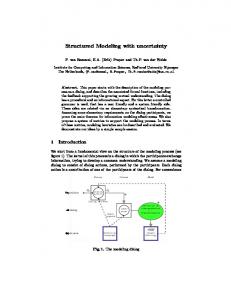
Figure 1. Complete Undirected Acyclic Graph (DAG) (Panel A), TETRAD-Generated Graph (Panel B), and Final DAG (Panel C) on Innovations from the First-Stage VAR Model and Soy-Related Variables.

38 November 2004


Table 1. VAR Model’s Correlation and Covariance Matrices and Correlation p-Values in Lower-Triangular Form. QBEANS (Y1)

PBEANS (Y2)

1.00 0.23

1.00

0.37 0.18 0.26 0.13

0.01 0.77 0.14 0.71

QMEAL (Y3)

PMEAL (Y4)

QOIL (Y5)

POIL (Y6)

1.00 -0.07 0.35 -0.08

1.00 0.05 0.35

1.00 0.08

1.00

0.000 0.463 0.000 0.368

0.000 0.592 0.000

0.000 0.362

0.000

p-Values for correlations 0.000 0.010 0.000 0.052 0.004 0.159

0.000 0.895 0.000 0.118 0.000

Note: Edges retained at the 10% significance level.

VAR model. Each of the elements are denoted as “rho” such that rho(1,3), or its symmetric equivalent rho(3,1), denotes the correlation between variables Y1 and Y3. The p-values for these correlations are provided in the second lower triangular matrix. Following recent DAG research, we chose a 10-percent significance level (Bessler and Akleman 1998, p. 1146; Babula, Bessler, and Payne 2004, p. 10). The following five undirected edges emerged from TETRAD II’s two stages of analysis on unconditional and conditional correlations:  QBEANS (Y1) – QMEAL (Y3): an undirected edge where soybean quantity and soy meal quantity are interrelated. Rho(3,1) equals +0.37 with a p-value of nearly zero (rounded to the third place and far below the chosen significance level of 0.10). This edge has two observational equivalents: Y1 Y3 or Y3 Y1.  PBEANS (Y2) – PMEAL (Y4): an undirected edge where soybean and soy meal prices are interrelated. Rho (4,2) equals +0.77, with a p-value of 0.00 (below the 0.10). This edge’s two observational equivalents are Y2 Y4 and Y4 Y2.  PBEANS (Y2) – POIL (Y6): an undirected

edge where soybean and soy oil prices are interrelated. Rho (6,2) equals +0.71 and has a p-value of 0.000 (below 0.10). This edge’s two observational equivalents are Y2 Y6 and Y6 Y2. � QMEAL (Y3) – QOIL (Y5): an undirected edge where soy meal and soy oil quantities are interrelated. Rho(5,3) equals +0.35, and has a p-value of 0.000 (below 0.10). This edge’s two observational equivalents are Y3 Y5 and Y5 Y3.  PMEAL (Y4) – POIL (Y6): an undirected edge where soy meal and soy oil prices are interrelated. Rho (6,4) equals +0.35 and has a p-value of 0.000 (below 0.10). This edge’s two observational equivalents are Y4 Y6 and Y6 Y5. Given these five TETRAD-suggested and undirected, there are 32 competing and observationally equivalent six-equation systems of contemporaneous correlations.16 The challenge is to choose the To conserve space, these 32 six-equation systems are not provided here, but are available on request from the authors. We have 6 variables, twice as many as Haigh and Bessler’s model. Unfortunately, there is no easy computational formula 16



optimal system of six equations from the 32 systems which best fit the data. Haigh and Bessler’s (2004) adaptation of Schwarz’s (1978) loss metric resolves the problem of choosing among the 32 competing but theoretically consistent systems of contemporaneous causal relations. Since we focus on causality relationships in contemporaneous time, contemporaneous relationships may be expressed in regression form and using the innovation estimates generated by the six equations of the first-stage VAR model.17 Each of the 32 systems of six causal relationships were expressed in regression form, estimated, and then scored by Haigh and Bessler’s (2004) adapted Schwarz loss metric.18 We selected the following system which minimized Haigh and Bessler’s adapted form of the Schwarz loss metric (the non-constant regressors and dependent variables refer to the first-stage VAR residuals): (2) (3) (4) (5) (6) (7)

QBEANS = f (CONSTANT, QMEAL) PBEANS = f(CONSTANT) QMEAL = f(CONSTANT) PMEAL = f(CONSTANT, PBEANS, POIL) QOIL = f(CONSTANT, QMEAL) POIL = f(CONSTANT, PBEANS).

to give the number of DAGs to score for N vertices (variables). In Haigh and Bessler (where N=3) 25 DAGs were scored, where all possible subgraphs are considered. In our case, and with our VAR of double the size, scoring all possible systems was deemed unnecessary, and another recent application in the literature provided guidance: that is, we only score edges that TETRAD left undirected (see Figure 1 Panel b). Thirty-two such systems consistent with the undirected edges or lines generated by TETRAD emerged to be scored with Schwarz’s loss metric. We followed Babula, Bessler, and Payne’s (2004) methods of scorable system selection. 17 For example, consider Y1 and Y2. That Y1 causes Y2 in contemporaneous time may be expressed as a regression of the innovations of Y1 against those of Y2 and a constant. Likewise, Y2’s causality of Y1 in contemporaneous time is expressed as a regression of Y2’s innovations against those of Y1 and a constant. Also, a variable is expressed as exogenous in contemporaneous time by regressing its innovations solely against a constant. See Haigh and Bessler (2004). 18 Haigh and Bessler (20043) adapted Schwarz’s loss metric as SL* = log (*) + k*log(T)/T, where * is a diagonal matrix with diagonal values of the variance/covariance matrix associated with a linear representation of the disturbance terms from an acyclic graph fit to the innovations for a VAR model.

Equations 2–7 are alternatively expressed diagrammatically as the DAG in Panel c of Figure 1, and were imposed on the first-stage VAR to form the DAG/Bernanke VAR model.19 Summarily, we began with a set of undirected edges (Figure 1, Panel a) which generated perhaps scores of competing, theoretically sanctioned systems of edges; we reduced this number down to 32 competing systems of six contemporaneously correlated relationships using TETRAD II and applied Haigh and Bessler’s adapted Schwarz (1978) loss metric to render the one system of the 32 which optimized the metric. As a result, we do not rely on arbitrary choice in choosing among the 32 competing systems of causal relationships. This method satisfies Pesaran and Shin’s (1998) goal of finding a method that delivers one unique ordering. Doan’s (1996, p. 8.10) methods provide a likelihood-ratio test of how well the imposed DAG-suggested system of contemporaneously causal relations are consistent with the data (Figure 1, Panel c). With Doan’s likelihood-ratio test value of 18.6 falling below the critical chi-square value of 23.2 (10 degrees of freedom), evidence at the 1-percent level is insufficient to reject the null hypothesis that the contemporaneous correlations that emerged from the TETRAD II and Haigh/Bessler analyses are consistent with the data. The imposed system of 19 We make a point here in response to a concern raised by a reviewer. Figures 1b and 1c may lead one to erroneously conclude that there is a disconnect in causality between the three prices and three quantities as separate groups. But one must realize that this is a graph of causal relationships in contemporaneous time only—say, at the very short-run horizons of 6 months or less, when overall quantity of soybeans (and hence aggregate potential supplies of QMEAL and QOIL) cannot appreciably change until the next set of planting decisions and harvests from the northern and southern hemisphere suppliers (occurring at opposing points in the calendar year). In this very short-run sense, quantities may not be expected to appreciably respond to prices until the next planting decision can be made—six or so months in the future. But overall in the model, as seen later from the impulse-response simulations and FEV decomposition patterns, there is a rich price-quantity interplay of influence among the model’s quantity and price variables that escalates as the time horizon increases. These impulse-response and FEV decomposition tools combine into a total pattern of causality: causal relationships serially over time through the seven-lag structure with the contemporaneous causality from directed edges in Figure 1c. In short and in total, the contemporaneous correlations in Figure 1c are only part of the causality story, and serial and contemporaneous correlations combine to generate a rich interplay among the model’s quantities and prices.

40 November 2004

orderings of the VAR variables in contemporaneous time and the sample appear compatible. Analysis of Impulse Responses from Increases in Soy Meal and Soybean Prices An important tool of VAR econometrics useful in applied work is the impulse-response function that simulates over time the effects of a one-time shock in one of the system’s series on the other endogenous variables in the system (Bessler 1984, p. 111; Hamilton 1994, ch. 11). This is done by converting the VAR model into its moving average (MA) representation, the parameters of which are complex combinations of the VAR regression coefficients (Bessler 1984, pp. 113–114). We chose to shock the impulse-response function twice: an increase in PMEAL and in PBEANS. These shocks are presumed to arise from a BSE-induced shift toward soy meal feed ingredients and/or from recordhigh current world import demand for soy meal’s prime ingredient, soybeans. The impulse responses of the respondent variables provide a map of sorts on how the soy-based markets respond to the shock (Goodwin, McKenzie, and Djunaidi 2003, p. 486). More specifically, examination of a simulation’s impulse responses illuminates the dynamic nature and patterns of monthly responses when a shock is placed on one of the chosen endogenous variables (here PMEAL, PBEANS) (Babula, Bessler, and Payne, p. 12). The dynamic results which emerge from the patterns of monthly impulses are reaction times required for the monthly impulses to begin, direction of impulses (increases or decreases), pattern of monthly impulse responses, and an elasticity-like multiplier of response showing the degree of ultimate respondent-variable reaction. Having estimated the DAG/Bernanke VAR in natural logarithms, shocks to, and impulse responses in, the logged VAR variables approximate proportional changes in the non-logged series (Babula, Bessler, and Payne 2004, p. 12). Using literatureestablished methods, a separate set of multipliers is calculated from the statistically non-zero impulse responses for each of the two simulations of the DAG/Bernanke VAR.20 A separate set of five respondent-variable multipliers are calculated for each of the two price-shock simulations. For a particular simulation’s impulses for a respondent variable, one sums the impulse responses into a cumulative proportional 20


Such multipliers have been calculated with those impulse responses that have likely achieved statistical significance at a chosen level of significance. Bessler, Yang, and Wongcharupan (2002, p. 819) noted that the DAG/Bernanke VAR and Bernanke’s structural VAR methods are confronted with a procedural shortcoming: there is not yet a widely available method of determining which of a respondent variable’s impulses are statistically non-zero at a chosen significance level. This is crucially important because often only a subset of a respondent variable’s calculated impulses likely achieves statistical significance at levels of 10 percent or less, and reliable multipliers calculated with only the statistically non-zero impulses can generate a response multiplier for the respondent variable which markedly differs from that calculated with longer streams of both significant and insignificant impulses. Packages such as Doan’s (1996) RATS have long-provided routines for imposing the Monte Carlo methods of Kloek and Van Dijk (1978) to discern statistical significance of impulses generated by Choleski-ordered VAR models. While calculating standard errors for impulses (to discern impulse significance) generated by Choleski-ordered models is a straightforward task, Bessler, Yang, and Wongcharupan (2002, p. 812) and Babula, Bessler, and Payne (2004, p. 12) note that such calculations for a DAG/Bernanke structure are far more challenging and beyond the scope of their studies. We follow these two studies’ lead and leave to future research the provision of such Monte Carlo methods for discerning which DAG/Bernanke VAR impulses are significant. We follow recent literature-established procedures and use simulation results from alternatively modeling the three-market, soy-based system as a Choleskiordered VAR to aid in discerning which subset of each respondent variable’s impulses generated by the DAG/Bernanke simulations were relevant to change in the respondent variable, sums the corresponding impulses in the shock variable into a cumulative proportional change and then divides the respondent variable’s cumulative change by the cumulative-shock-variable change. The result is an elasticity-like multiplier that provides what has been interpreted as a long-run average percentage change in the respondent variable per percentage point change in the shock variable. Unlike an elasticity, it is reduced-form in nature and not defined for a particular point in time. These methods are summarized in Goodwin, McKenzie, and Djunaidi (2003, p. 486) and Babula, Colling and Gajewski (1994).



the calculation of response multipliers.21 These and other dynamic results are provided in Figures 2 and 3 and in Table 2.22 The separately imposed increases in PMEAL and PBEANS on the DAG/Bernanke VAR were presumed to arise from BSE-induced increases in soy meal demand as feed ingredients and historically high and escalating world demands for soy meal’s main ingredient, soybeans. Recent VAR econometric research on U.S. commodity markets established that there is some subjective leeway in identifying the source of shocks for this (or any) reduced form model (Babula, Bessler, and Payne 2004, p. 14; Babula and Rich 2001, p. 10). The two price increases could have arisen from other sources—perhaps a supply-side event such as decreased production or from a change in consumer demand. However, our presumed sources of the shocks are valid.23 21 We alternatively modeled our six-equation first-stage VAR model with a Choleski decomposition, applied Kloek and Van Dijk’s well-known Monte Carlo methods to our simulations of increasing shocks in PMEAL and PBEANS, and noted that in no case did monthly impulses achieve statistical significance beyond about one year. In order to be flexible, and given the differences in the degree of restrictiveness of the DAG/Bernanke and Choleski orderings, we calculated the response multipliers for the impulse responses generated for horizons through 18 months. For want of Monte Carlo methods applicable to DAG/Bernanke and Bernanke structural VARs, we followed recent literature-established procedures (see Babula, Bessler, and Payne 2004, p. 13) and used related— though not strictly comparable—Choleski VAR impulses to discern the statistically non-zero subsets of each respondent variable’s impulses with which to calculate the response multipliers. Any impulses comprising assumed reaction times in the response patterns were not included in the multiplier calculations provided later in the paper.

The one-time shocks imposed were orthogonalized standard-error increases of 2.4 percent for PMEAL and 2.7 percent for PBEANS. However, it is well known that for such double-logged and linear VAR models, the shock size and shock sign is arbitrary. For example, the impulse-response simulations of a 20-percent shock are obtained by simply multiplying the impulses from simulating a 10-percent shock by the scalar 2.0. Likewise, the impulses generated from simulating a 10-percent decline in a shock variable are obtained by simply multiplying the impulses generated from a 10 percent positive shock by the scalar -1.0. See Babula, Colling, and Gajewski (1994, p. 377). 22

23 For example, Babula, Bessler, and Payne (2004, pp. 10–11) estimated a similar model for U.S. wheat-based markets. They imposed a rise in wheat price on the model and presumed it to be tariff-induced (imported and domestic wheat consignments were shown as likely substitutable). They

Price-Induced Impacts on the U.S. Soybean Market Overall, evidence, theory, market knowledge, and alternative modeling results suggest that there is likely a six-month lag before QBEANS begins reacting to either price shock. This is because market-clearing soybean quantity, as defined, is likely fixed at very short-run horizons.24 Monthly impulses in soybean quantity induced by the PMEAL and PBEAN increases are quantity declines. Given that the model is reduced-form in nature, these negative impulses suggest that the quantity-decreasing demand effects overwhelm the quantity-increasing supply effects such that the two imposed shocks in acknowledged that the rise in wheat price could have arisen from other sources as well: from changes in production costs or in domestic demand. 24 Figures 2 and 3 suggest that during the first six months there were a number of positive and negative impulses in QBEANS. The first six QBEANS impulses from both simulations are largely pattern-less relative to the remainder of the two total patterns. After six months, both QBEAN impulse patterns take on clear and well-defined patterns. Owing to the above-noted lack of Monte Carlo procedures to generate impulse standard errors, we are unable to discern which of these first six QBEANS impulses from either simulation are statistically zero or non-zero. However, overall DAG/Bernanke evidence, theory, market knowledge, and results from alternatively modeled VAR models of the same system suggest that we should assume these first six impulses in each simulation to be statistically zero or insignificant. First, QBEANS was defined from USDA, ERS (1993–2004b) situation and outlook data as a reducedform, market-clearing soybean quantity that is largely fixed at short-run horizons of a half-year or less. This is because soybeans are an annual crop grown in both the northern and southern hemispheres, which have opposing growing seasons and harvests. Unless augmented U.S. soybean imports should markedly overwhelm an export decline, which is historically unlikely, then QBEANS is likely to be largely fixed at very short-run horizons of about 6 months or less. Second, and perhaps most importantly, as seen from the ensuing analysis of FEV decompositions, variation in both PMEAL and PBEANS contribute little to the explanation of QBEANS behavior at horizons of six months or less, leading to our conclusion that the first six QBEANS impulses in both scenarios are likely statistically zero. Third, we estimated our VAR system as a Choleski-ordered VAR, simulated it twice under PMEAL and PBEANS increases, applied Kloek-VanDijk’s Monte Carlo simulations to both simulations’ impulses, and generated results that suggest that all or most of the first six QBEANS impulses from both simulations were statistically zero at the 5% and 10% significance levels. As a result, we assumed sixmonth reaction times for the first six QBEANS impulses from both simulations.

42 November 2004


Panel A: Impulse responses in the soybean and soy meal markets.

Panel B: Impulse responses in the soyoil market.

Figure 2. Monthly Impulse Responses in Soy-Based Markets to a Rise in Soy Meal Price.



Panel A: Impulse responses in the soybean and soy meal markets.

Panel B: Impulse responses in the soyoil market.

Figure 3. Monthly Impulse Responses in Soy-Based Markets to a Rise in Soybean Price.

Responses in soybean price (PBEANS) from:

Responses in soy meal quantity (QMEAL) from:

Responses in soy meal price (PMEAL) from:

Responses in soy oil quantity (QOIL) from:

Responses in soy oil price (POIL) from:

Cycles toward zero -0.80

Pattern, monthly impulses

Response multiplier

-0.20

Cycles toward zero

Decline

6

+1.70

Bellshaped

Increase

3

Shocked

Shocked

Shocked

Shocked

-0.50

Cycles toward zero

Decline

0

-0.10

Cycles toward zero

Decline

0

Shocked

Shocked

Shocked

Shocked

+0.52

Cycles to zero

Increase

0

-4.60

Bellshape

Decline

0

-0.41

Bellshaped

Decline

0

+4.0

Bellshaped

increase

0

+1.25

High then lessening

Increase

0

Notes: Response multipliers provide a percentage change in the respondent variable per percentage point change in the shock variable. Sign does not necessarily denote direction of change, but rather the relationship of the response to shock variable movements: a positively (negatively) signed multiplier signifies responses that are similarly (oppositely) directed with movements in the shock variable.

Decline

6

PMEAL PBEANS PMEAL PBEANS PMEAL PBEANS PMEAL PBEANS PMEAL PBEANS PMEAL PBEANS increase increase increase increase increase increase increase increase increase increase increase increase

Responses in soybean quantity (QBEANS) from:

Response direction

Reaction times (months)

Dynamic Aspect

Table 2. Dynamic Aspects and Multipliers of Respondent Variables from Positive Shocks in Soybean and Soy Meal Prices.

44 November 2004 Journal of Food Distribution Research 35(3)



increased PMEAL and PBEANS result in a lesser market-clearing quantity for soybeans. The declines in soybean quantity from both simulations take on a multicyclical pattern where cycles dampen toward zero over time (Table 2, Figures 2 and 3). As expected, QBEANS responds more markedly, rapidly, and with more volatility to a shock in ownprice (PBEANS) than in PMEAL downstream. On average historically, QBEANS has declined by 0.8 percent for each percentage rise in PBEANS, and by a far lesser 0.2 percent for each percentage rise in PMEAL (Table 2). On average historically, the PMEAL increase has elicited similarly directed increases in PBEANS. The soybean price impulses commence after a threemonth reaction time, take on a roughly bell-shaped pattern over time, and ultimately reflect PBEAN increases of 1.7 percent for each percentage rise in PMEAL. A PBEANS multiplier in excess of unity is not surprising given that any quantity of soybeans yields about 76 percent volume of meal, such that each percentage change in soy meal is associated with 1.3 percent change in soybeans.25 Price-Induced Impacts on the U.S. Soy Meal Market A rise in PMEAL elicits a series of generally declining QMEAL responses (Figure 2).26 As with QBEANS impulses, the market-clearing soy meal quantity seems to decline as the reduced-form model’s quantity-decreasing demand effects from the two price shocks outweigh the supply side’s quantity-augmenting effects. PMEAL-induced declines in QMEAL begin during the same month (within 29 days) of the shock; take on a shallow, bell-shaped pattern that decays over time towards 25 From USDA Agricultural Marketing Service (2004, p. 3) data, each 60-pound bushel yielded 11.06 pounds of soy oil (18.4%), 45.86 pounds of soy meal (76.4%), and 3.08 pounds of other materials (5.2%). 26 Generally, while QMEAL responds negatively to PMEAL, there are three positive but negligibly valued, impulses within the very short-run set of horizons of six months or less. These could be short-run responses in the QBEANdefining components from the imposed price shock. Perhaps QMEAL rises from a brief rise in QMEAL supply or from a sudden surge in imports in soy meal and/or soybeans slated for crushing induced by the PMEAL shock. At longer-run horizons beyond a single crop-adjustment period (about six months, as noted previously), QMEAL impulses are generally negative.

zero; and ultimately reflects QMEAL declines of 0.5 percent for each percent rise in PMEAL (Table 2, Figure 2). A PBEANS increase elicits monthly QMEAL declines that take-on a shallow, bell-shaped pattern that decays toward zero with time, and PMEAL increases that are initially pronounced and which thereafter decay. On average historically, each percentage rise in PBEANS elicits a 0.1 percent decline in QMEAL, and a 0.5 percent rise in PMEAL. Price-Induced Impacts on the U.S. Soy Oil Market There are rather immediate, notable, and pronounced downstream effects of increases in PMEAL and PBEANS on the soy oil market. Some of the multipliers of soy oil market-variable response far exceed unity in absolute value. Because soy oil accounts for only 18 percent of soybean volume, which is far less than meal’s 76-percent share, movements in the soybean and meal markets are typically associated with larger-percentage oil-market changes. Patterns of POIL and QOIL impulses from both price shocks are generally smoother than other soybased market impulse patterns, and bell-shaped with ultimate response decay towards zero over time. Soy oil is highly competitive with and substitutable for other vegetable oils (e.g., rapeseed and palm oils) in a wide variety of food and industrial uses. As a result, responses in soy oil price and quantity take on rapidly unfolding patterns that are gradual and time-enduring. On average historically, each percentage rise in soy meal price has generated a far-greater-than-proportional 4.6 percent decline in QOIL and 4.0 percent rise in POIL; each percentage rise in PBEANS has elicited a 0.4 percent fall in QOIL and a 1.3 percent rise in POIL. Soybean oil, although the leading vegetable oil in the world, accounts for only one third of world production of vegetable oil, and for less than one fifth of world production of all “fats and oils” (combined vegetable oils and all animal fats, including tallow, fish oil, butter and lard).27 Moreover, subDuring 2003/2004, soybean oil production accounting for 32 percent of the world production of 100 million metric tons (mmt) of major vegetable oils, while palm oil accounted for 28 percent, rapeseed oil for 14 percent, and “other” oils for 26 percent (USDA FAS 2004b). Worldwide soybean oil production represented 18 percent of the 129 mmt of major vegetable oils, animal fats, fish oil, and butter (all fats and oils) (Oil World 2004). 27

46 November 2004

stitution among vegetable oils and most animal fats is high, and prices highly correlated (Gould, Box, and Perali 1991). This degree of competition may help explain the large supra-unity absolute values of most of the soy-oil market response multipliers in Table 2. Contrasted to soybean oil, soybean meal accounted for 70 percent of world protein meal production in 2003/2004 (USDA FAS 2004b). Moreover, although other oilseed meals or feed grains (e.g. wheat) can be substituted for soybean meal in some animal feeds, the amount of substitution is limited by technical and functionality factors such as maximal fiber content or protein requirements (Bickerton and Glauber 1990, pp. 9–11). Thus there are fewer direct-substitute oilseed or protein meals for soybean meal, and this is reflected in the low price inelasticity of demand for soybean meal with regard to changes in the price of other oilseed meals.28 Analysis of Forecast Error Decompositions Analysis of forecast error variance (FEV) decompositions is a well-known accounting method for residuals or innovations (Bessler 1984, p. 111; Sims 1980). Such analysis is closely related to Granger causality analysis. While both tools provide evidence of causal relations among two variables, analysis of FEV decompositions provides well-known extensions to Granger causality tests (Babula, Bessler, and Payne 2004, p. 15). A modeled endogenous variable’s FEV is attributed at alternative (here monthly) horizons to shocks in each endogenous variable (including itself). As a result, analysis of FEV decompositions not only provides evidence of the simple existence of a causal relationship among two variables, but it also illuminates the strength and dynamic timing of such a relationship (Saghaian, Hassan, and Reed 2002, p. 107; Bessler 1984, p. 111). Table 3 provides the FEV decompositions of the DAG/Bernanke VAR model of six soy-based variables. Such decompositions reflect the causal relations embedded in both the model’s seven-order lag structure over time, as well as the DAG-suggested contemporaneous 28 The U.S. own-price elasticity of demand for soybean meal was found to be -0.31. The U.S. price elasticity of demand for soybean meal with respect to the price of other oilseed meals was estimated at +0.05, indicative of a demand substitutability, although very inelastically so. See Gardiner, Roningen, and Liu (1989).


causal relationships which emerged from applying the methodologies of Bessler and Akleman (1998) and Haigh and Bessler (2004). A variable is considered exogenous (endogenous) when large (small) proportions of its FEV are attributed to its own movements (that is, to own-variation). Likewise, a variable’s endogeneity is suggested when large proportions of its FEV are attributed to variation in the system’s other endogenous variables (Bessler 1984; Goodwin, McKenzie, and Djunaidi 2003, pp. 488–489). Decompositions of two or more variables may be summed at a particular horizon for a “collective” effect—for example, at a chosen horizon the collective effect of the three soy-based prices on one of the modeled soy-based quantities can be summed and examined. The quantity of soybeans is highly exogenous at horizons of six months or less, when from 62 to 84 percent of its behavior is attributed to ownvariation. Beyond six months, QBEANS becomes more endogenous, with more than half of its variation explained by the collective movements of the five other VAR variables. Soybean quantity appears most influenced by its own market workings, with moderate influences arising from downstream price and quantity movements. At horizons of 12 months and beyond, the explained proportions of QBEANS’ behavior are attributed as follows: 61 to 69 percent collectively by its own market workings (PBEANS and QBEANS), and from 25 to 33 percent collectively to all three prices (PBEANS, PMEAL, and POIL). Soybean price appears exogenous at horizons of 18 months or less, when no less than 73 percent of PBEANS’ variation is self-attributed. PBEANS rapidly takes on an increasingly endogenous role as time progresses: after horizons of 18 months, own-variation’s explanation of soybean price’s behavior drops to low as 24 percent. QBEANS’ direct explanation of soybean price seems minimal at all reported horizons. However, PBEANS appears indirectly influenced by combined movements in own-market variables (itself and QBEANS): these two variables influence the behavior of variables in the two downstream co-product markets for soy meal and soy oil, which in turn noticeably contribute to the explanation of PBEANS behavior. At horizons beyond 18 months, the proportions of PBEANS’ FEV attributed to the workings of the soy meal market reach a collective 46 percent (PMEAL



Table 3. Decompositions of Forecast Error Variance Generated by the Soy-Based DAG/Bernanke VAR. Percentage of forecast error variance explained by Variable explained

Monthly horizon

QBEANS

PBEANS

QMEAL

PMEAL

QOIL

POIL

QBEANS

1 2 4 6 12 18 24 30 36 48 60

83.33 75.40 66.94 61.61 56.44 52.46 50.49 49.93 49.40 48.83 48.54

1.43 6.18 8.53 9.42 12.70 13.41 13.38 13.33 13.09 12.89 12.88

12.49 16.12 15.16 17.52 15.44 15.53 14.94 14.96 14.86 14.08 14.81

0.11 0.11 2.55 2.54 6.90 7.19 9.80 10.30 10.94 11.48 11.68

1.46 1.33 1.77 3.21 3.09 3.57 3.66 3.79 3.93 4.03 4.02

0.08 0.87 5.05 5.70 5.43 7.83 7.73 7.68 7.78 7.96 8.08

PBEANS

1 2 4 6 12 18 24 30 36 48 60

1.29 0.96 1.62 2.66 4.09 3.57 3.47 3.72 3.56 2.95 2.41

97.09 96.09 88.40 85.15 77.64 73.27 66.24 56.32 45.80 29.78 23.80

0.62 2.07 5.60 6.61 6.76 5.96 4.85 3.94 3.37 3.45 4.18

0.00 0.00 1.65 2.42 6.93 11.01 15.80 22.06 28.16 38.00 41.86

0.74 0.54 2.43 2.54 3.04 4.64 8.29 11.92 14.62 15.28 13.58

0.26 0.34 0.31 0.61 1.55 1.55 1.35 2.05 4.5 10.55 14.19

and QMEAL), proportions of FEV attributed to the collective workings of the soy oil market reach 28 percent, and proportions of FEV collectively attributed to the workings of both downstream markets reach more than 70 percent. However, movements in the three modeled quantities have a modest effect on PBEANS and collectively explain no more than 22 percent of PBEANS’ variation at the reported horizons. Therefore, the U.S. soybeans market at the farmgate appears primarily driven by the downstream workings of the two markets for soybeans’ two co-products.

Soy meal quantity is exogenous at short-run horizons of six months or less, when from 72 to 98 percent of its behavior is attributed to ownvariation. As horizons lengthen beyond six months, QMEAL behavior is decreasingly explained by own-variation, and increasingly explained by ownprice (PMEAL). Prices heavily influence QMEAL behavior at horizons of 12 months or more: ownprice explains up to 25 percent, while the three modeled soy-based prices collectively explain up to 47 percent of QMEAL’s variation. QBEANS and QOIL variation have modest influence on soy meal

48 November 2004


Table 3. Decompositions of Forecast Error Variance Generated by the Soy-Based DAG/Bernanke VAR – Continued. Percentage of forecast error variance explained by Variable explained

Monthly horizon

QBEANS

PBEANS

QMEAL

PMEAL

QOIL

POIL

QMEAL

1 2 4 6 12 18 24 30 36 48 60

0.23 1.51 2.58 3.33 10.85 10.06 9.78 9.19 8.81 8.69 8.80

1.58 2.21 7.08 12.49 13.32 13.51 13.66 12.96 12.19 12.38 14.16

98.04 95.38 80.58 71.54 57.30 49.35 43.84 40.76 38.78 37.53 35.37

0.08 0.25 5.86 5.63 10.49 14.04 18.99 21.84 24.25 25.02 24.65

0.04 0.21 2.07 4.98 5.60 6.84 7.22 7.74 7.68 7.47 8.51

0.02 0.43 1.83 2.01 2.45 6.20 6.51 7.52 8.29 8.90 8.52

PMEAL

1 2 4 6 12 18 24 30 36 48 60

2.29 2.32 2.55 3.18 3.48 3.10 3.96 5.30 5.62 4.11 2.98

63.22 63.48 58.30 54.64 44.86 42.20 41.78 38.03 30.65 18.13 12.86

0.60 0.53 2.24 2.50 2.87 2.97 2.71 2.10 1.68 2.17 3.32

24.39 21.90 23.67 22.46 16.67 15.29 14.05 16.62 24.11 38.14 44.15

0.45 0.66 0.91 0.99 1.09 1.72 5.79 12.64 16.97 17.16 14.51

9.06 11.12 12.33 16.24 31.04 34.73 31.71 25.31 20.97 20.29 22.18

quantity, with neither explaining more than about 11 percent of QMEAL variation at horizons of 12 months or beyond. QMEAL appears more influenced by movements in price than than by quantity movements. Soy meal price is endogenous at all reported horizons: own-variation accounts for as little as 14 percent and for no more than 44 percent of its behavior at all reported horizons. Soybeans price heavily influences PMEAL and explains from 55 to 63 percent of PMEAL’s FEV at horizons of six months or less. Soy meal price is noticeably influenced by soy oil price, with from 20 to 35 percent of

PMEAL behavior attributed to variations in POIL at horizons of a year or more. Generally, movements in the three soy-based quantities have moderate effects on PMEAL, with the collective movements in all three quantities explaining from seven to no more than 24 percent of PMEAL variation at horizons at and surpassing 12 months. Soy oil quantity is also exogenous at shorter-run horizons of six months or less when own-variation explains from 58 to 84 percent of QOIL behavior. At horizons of 12 months or more, QOIL becomes increasingly endogenous with own-variation explaining from 40 percent to as little as 16 percent



Table 3. Decompositions of Forecast Error Variance Generated by the Soy-Based DAG/Bernanke VAR – Continued. Percentage of forecast error variance explained by Variable explained

POIL

Monthly horizon

QBEANS

PBEANS

QMEAL

PMEAL

QOIL

POIL

2 4 6 12 18 24 30 36 48 60

2.63 4.16 7.53 8.25 6.14 4.43 3.41 2.94 3.90 5.00

2.78 5.71 7.95 7.41 6.16 4.86 3.68 3.50 9.17 15.28

10.67 11.57 11.12 4.65 3.57 3.71 4.16 4.74 5.09 3.41

11.53 11.28 12.62 27.41 36.84 42.26 45.88 47.20 42.57 39.23

69.53 64.55 58.03 39.97 28.53 22.62 18.86 16.48 16.06 19.23

2.86 2.73 2.76 12.31 18.76 22.12 24.00 25.14 23.22 17.86

1 2 4 6 12 18 24 30 36 48 60

0.45 2.11 6.26 7.15 8.13 6.62 6.17 6.09 6.17 6.21 6.18

42.10 40.54 41.55 44.61 44.34 41.25 39.26 38.36 38.19 38.34 38.21

0.90 3.76 3.94 3.34 2.55 2.21 2.12 2.17 2.21 2.25 2.22

0.07 0.30 1.88 3.33 12.82 21.46 25.55 27.07 27.28 27.17 27.37

0.10 0.51 3.53 3.25 3.66 3.73 3.80 3.80 3.78 3.81 3.99

56.38 52.77 42.84 38.32 28.49 24.74 23.09 25.52 22.37 22.22 22.03

of its behavior. As with QMEAL and QBEANS, soy oil quantity is heavily influenced by soy-based prices, especially at the longer-run horizons. At horizons of 12 months or beyond, own-prices (POIL) explains as much as 25 percent of QOIL behavior, while movements in the three prices collectively explain as much as 76 percent of QOIL behavior. Other soy-related quantities contribute negligibly to explaining QOIL behavior, with neither QBEANS or QMEAL explaining more than about 8 percent of QOIL variation at horizons of 12 months and beyond. QMEAL also seems more driven by prices than by quantities.

Soy oil price is generally endogenous at longerrun horizons: own-variation explains from 38 to 56 percent of POIL behavior at horizons below 12 months, and no more than 28 percent at horizons at and exceeding 12 months. The other two soy-based prices heavily influence POIL’s behavior at horizons beyond six months, when PBEANS explains up to 44 percent and PMEAL explains up to 27 percent of POIL’s variation. Modeled soy-based quantities collectively explain only from 12 to 14 percent of POIL’s behavior at all reported horizons. Overall, the FEV decompositions suggest that the three prices appear to drive the three-market

50 November 2004

soy-based system more than do quantities. Collectively, the three soy-based prices explain up to nearly half (47 percent) of QMEAL behavior, while the three soy-based quantities collectively explain no more than 24 percent of PMEAL variation. For the soybeans market, the three prices collectively explain up to about 33 percent of QBEANS behavior, while the three quantities collectively explain no more than 22 percent of PBEANS behavior. Such price-dominated influences are particularly evident from patterns of soy oil FEV decompositions. While the three prices collectively account for as much as 76 percent of QOIL variation, the three quantities collectively explain no more than about 14 percent of soy oil price behavior. There is some mutual support of the impulseresponse results from two imposed price shocks (increases in PMEAL, PBEANS). The FEV decompositions in Table 3 suggest that at the very short-run horizons (six months or less), PMEAL and PBEANS contribute modestly or negligibly to the explanation of the behavior of soybean and soy meal quantities. These FEV decompositions reinforce our assumptions that in both simulations the first six impulses are likely statistically zero and form a half-year reaction time for QBEANS and are unimportant (and perhaps statistically insignificant) for QMEAL. At horizons of 12 months and beyond, the FEV decompositions in Table 3 suggest that both shock variables have a greater influence on the soy oil markets than on the soy meal and soybeans markets. These FEV results reinforce the impulse-response results in Figures 2 and 3 and in Table 2.29 Summary and Conclusions For perhaps the first time, we have applied the new DAG/Bernanke VAR methodology developed by Bessler and Akleman (1998) and Haigh and Bessler (2004) to the monthly upstream and downstream U.S. markets for soy-based products (soybeans, soy meal, soy oil). We have used the model to generate two sets of VAR econometric results that illuminate the empirical magnitudes of parameters that drive, 29 For example, results in Table 3 suggest that the combined variation of PMEAL and PBEANS explain the following percentages of FEV for modeled quantities at horizons of 12 months and beyond: 35–55 percent for QOIL, which exceeds 28–39 percent for QMEAL and 20–25 percent for PBEANS.


and the dynamic nature of the monthly interactions or linkages among, the U.S. soybean, soy meal, and soy oil markets. First are the impulse responses from simulating the model under two price shocks (increases in PMEAL and in PBEANS). The shocks to (increases in) soy meal and soybean prices were presumed to be the result of a BSE-induced rise in the price of soy meal as a feed ingredient and from continually escalating world demands for soybeans, soy meal’s primary ingredient. A number of elasticity-like and policyrelevant response multipliers emerged from both simulations. On average historically, each percentage rise in soy meal price elicited declines in market-clearing quantities of -0.8 percent for QBEANS, -0.5 percent for QMEAL, and -4.6 percent for QOIL, as well as increases of 1.7 percent and 4.0 percent in soybeans and soy oil prices, respectively. Likewise, each percentage rise in soybeans price elicited declines of -0.2 percent for QBEANS, -0.14 percent for QMEAL, and -0.41 percent for QOIL and increases of 0.52 percent and 1.25 percent in soy meal and soy oil prices, respectively. In the shorter-run horizons of one year or less, the prices and quantities of the three soy-based products are more exogenous than they are after one year, when the six-variable system increasingly and steadily integrates into a highly endogenous system. Generally, at horizons of one year or more prices seem to drive the system more than do quantities: PMEAL, PBEANS, and POIL appear to drive the three quantitites more than QBEANS, QMEAL, and QOIL drive the three prices. Nonetheless, there is a rich and escalating interplay of causal influences among prices and quantities, especially at horizons beyond six months. A positive shock in soy oil price would likely push prices of soybeans, soy meal, and soy oil higher. As a reduced-form model, the DAG/Bernanke VAR model suggests that the negative demand side effects will prevail over the positive supply side effects and result in decreases in all three marketclearing quantities. Soy oil appears to be the most influenced of the three markets by movements in PMEAL or movements in the two other markets. This high sensitivity of response is suggested by POIL’s and QOIL’s relatively high levels of endogeneity from FEV decompositions and the far-greater-than-unity POIL and QOIL response multipliers from imposing a PMEAL increase on the VAR. Such sensitivity



may arise from soy oil’s minor share (18 percent) of pre-crushed soy bean volume and from the high levels of soy oil competition with non-soy oils in a variety of industrial and consumer uses. References Babula, R., D. Bessler, and W. Payne. 2004. “Dynamic Relationships Among U.S. Wheat-Related Markets: Applying Directed Acyclic Graphs to a Time Series Model.” Journal of Agricultural and Applied Economics 36:1–22. Babula, R., P. Colling, and G. Gajewski. 1994. “Dynamic Impacts of Rising Lumber Prices on Housing-Related Prices.” Agribusiness: An International Journal 10:373–388. Babula, R. and K. Rich. 2001. “Time Series Analysis of the U.S. Durum Wheat and Pasta Markets.” Journal of Food Distribution Research 32(2): 1–19. Bernanke, B. 1986. “Alternative Explanations of the Money-Income Correlation.” CarnegieRochester Conference Series on Public Policy 25:45–100. Bessler, D. 1984. “An Analysis of Dynamic Economic Relationships: An Application to the U.S. Hog Market.” Canadian Journal of Agricultural Economics 32:109–124. Bessler, D. and D. Akleman. 1998. “Farm Prices, Retail Prices, and Directed Graphs: Results for Pork and Beef.” American Journal of Agricultural Economics 80(5):1144–1149. Bessler, D., J. Yang, and M. Wongcharupan. 2002. “Price Dynamics in the International Wheat Market: Modeling with Error Correction and Directed Acyclic Graphs.” Journal of Regional Science 42:793–825. Bickerton, T. And J. Glauber. 1990. World Oilseed Markets—Government Intervention and Multilateral Policy Reform. Washington, D.C.: U.S. Department of Agriculture, Economic Research Service. March. Dickey, D. and W. Fuller. 1979. “Distribution of Estimates for Autoregressive Time Series with a Unit Root.” Journal of the American Statistical Association 74:427–431. Doan, T. 2002. “Generalized Impulse Responses.” The RATSletter 15:4. Doan, T. 1996. RATS Users’ Manual, Version 4. Estima, Evanston, IL. Fuller, W. 1996. Introduction to Statistical Time

Series. New York: John Wiley & Sons. Gardiner, W., V. Roningen, and K. Liu. 1989. Elasticities in the Trade Liberalization Database. United States Department of Agriculture, Washington, D.C. Goodwin, H. L., Jr., A. McKenzie, and H. Djunaidi. 2003. “Which Broiler Part Is the Best Part?” Journal of Agricultural and Applied Economics 35(3)483–495. Gould, B., T. Box, and F. Perali. 1991. “Demand for Food Fats and Oils.” American Journal of Agricultural Economics 71:212–221. Granger, C. W. J. and P. Newbold. 1986. Forecasting Economic Time Series. Academic Press, New York. Gruen, J. 2004. “Creutzfeld-Jakob Disease.” http: //usaneurosurgery.com/glossary/i/jacob%creutz feld%20disease.htm. Retrieved April 14. Gullickson, Gil. (2004a) “Animal Proteins Continue to Crash; Other Ingredients Mostly Unchanged.” Feedstuffs Jan. 19:21. Gullickson, Gil. (2004b) “Blood Meal Restrictions, Avian Flue Push Corn, Soybean Futures Lower.” Feedstuffs Feb. 2:25. Haigh, M., and B. Bessler. 2004. “Causality and Price Discovery: An Application of Directed Acyclic Graphs.” Journal of Business forthcoming. Hamilton, J. 1994. Time Series Analysis. Princeton University Press, Princeton, NJ. Harris, R. 1995. Cointegration Analysis in Econometric Modeling. Prentice-Hall, New York. Harvey, A. 1990. The Econometric Analysis of Time Series. MIT Press, Cambridge, MA. Johansen, S. and K. Juselius. 1992. “Testing Structural Hypotheses in Multivariate Cointegration Analysis of the PPP and UIP for UK.” Journal of Econometrics 53:211–244. Johansen, S. and K. Juselius. 1990. “Maximum Likelihood and Inference on Cointegration: with Applications to the Demand for Money.” Oxford Bulletin of Economics and Statistics 52: 169–210. Jonnala, S., S. Fuller, and D. Bessler. 2002. “A GARCH Approach to Modeling Ocean Grain Freight Rates.” International Journal of Maritime Economics 4:103–125. Kloek, T. and H. VanDijk. 1978. “Bayesian Estimates of Equation System Parameters: An Application of Monte Carlo.” Econometrica 46:1–20.

52 November 2004

Kwiatowski, D., P. Phillips, P. Schmidt, and U. Shin. 1992. “Testing the Null Hypothesis of Stationarity Against the Alternative of a Unit Root: How Sure Are We that Economic Time Series Have a Unit Root?” Journal of Econometrics 54:159–178. McNeil, D., and D. Grady. 2004. “Ban Urged on All Animal Protein for Cattle.” New York Times News Service Feb. 5. www.nytimes.com/2004/ 02/05/national/nationalspecial2/05COW.html. Milling and Baking News. 2004. “HAS Expands Safeguards to guard against B.S.E. Transmission.” Feb. 3:20. Oil World. 2004. “BSE Concern in the USA.” Jan. 2:2. Patterson, K. 2000. An Introduction to Applied Econometrics: A Time Series Approach. Palgrave, New York. Pearl, J. 1995. “Causal Diagrams for Empirical Research.” Biometrica 82:669–710. Pesaran, H., and Y. Shin. 1998. “Generalized Impulse Response Analysis in Linear Multivariate Models.” Economic Letters 58:17–29. Pressler, M. 2004. “Steps to Safer Beef?” The Washington Post Jan. 18:F1. Reuters. 2004. “Expert Panel Sees More U.S. Mad Cow Cases,” New York Times News Service Feb. 4. http://www.nytimes.com/reuters/business/ business.madcow.html. Saghaian, S., M. Hassan, and M. Reed. 2002. “Overshooting of Agricultural Prices in Four Asian Economies.” Journal of Agricultural and Applied Economics 34(1):95–109. Scheines, R., P. Spirtes, C. Glymour, and C. Mee. 1994. TETRADII: Tools for Causal Modeling. Carnegie Mellon University, Pittsburgh, PA. Schwarz, G. 1978. “Estimating the Dimension of a


Model.” Annals of Statistics 6:461–464. Sims, C. 1988. “Bayesian Skepticism on Unit Root Econometrics.” Journal of Economic Dynamics and Control 12:463–474. Sims, C. 1980. “Macroeconomics and Reality.” Econometrica 48:1–48. Spirtes, P., C. Glymour, and R. Scheines. 2000. Causation, Prediction, and Search. SpringerVerlag, New York. Tiao, G., and G. Box. 1978. “Modeling Multiple Time Series: With Applications.” Journal of the American Statistical Association 76:802–816. U.S. Department of Agriculture, Agricultural Marketing Service. 2004. Grain and Feed Weekly Summary and Statistics 32(9). Feb. 27. U.S. Department of Agriculture, Economic Research Service 2004a. Oil Crop Outlook. April 9: Tables 8 and 10. U.S. Department of Agriculture, Economic Research Service . 1993–2004b. Oil Crops Situation and Outlook Yearbook, various annual issues. U.S. Department of Agriculture, Foreign Agricultural Service 2004a Oilseeds, FOP 03-04. March: Table 5. U.S. Department of Agriculture, Foreign Agricultural Service 2004b. Oilseeds: World Markets and Trade. March: Table 3. U.S. Department of Agriculture, Foreign Agricultural Service 2004c. 2004. Oil Crops Outlook. September 13: Table 10. U.S. Department of Agriculture, Office of the Chief Economist. 2004. World Agricultural Supply and Demand Estimates. April. http://usda.mannlib.c ornell.edu. Retrieved April 21. U.S. Department of Agriculture, World Outlook Board.2004. Agricultural Supply and Demand Estimates. Feb. 10:26. Vendantam, S. 2004. “Ban on Meat from Downers Grows.” The Washington Post Jan. 27:A3. Weintraub, A. 2004. “A Bum Steer on Mad Cow Disease.” Business Week Jan. 12:39.

Modeling US Soy-Based Markets with Directed ... - Semantic Scholar

Modeling US Soy-Based Markets with Directed ... - Semantic Scholar

Suggest Documents

modeling us soy-based markets with directed acyclic graphs ... - USITC

Scaffolding Self-directed Learning with ... - Semantic Scholar

Modeling Directed Obligations and Permissions in ... - Semantic Scholar

Goal-Directed Modeling of Self-adaptive Software ... - Semantic Scholar

The Trouble With Electricity Markets - Semantic Scholar

ASEAN-5 + 3 and US Stock Markets ... - Semantic Scholar

Modeling and asset allocation for financial markets ... - Semantic Scholar

Flow-directed Inlining - Semantic Scholar

US Markets Construction Overview

Supporting Creativity with Conceptual Modeling ... - Semantic Scholar

Modeling Documents with Event Model - Semantic Scholar

Modeling Cognition with Software Agents - Semantic Scholar

implicit modeling with procedural techniques - Semantic Scholar

Modeling Electric Discharges with Entropy ... - Semantic Scholar

Complex Systems Modeling with Cellular ... - Semantic Scholar

Modeling Learner Affect with Theoretically ... - Semantic Scholar

Tool Modeling with Fujaba - Semantic Scholar

Modeling Disjunctive Constraints with a ... - Semantic Scholar

Multidimensional Modeling with UML Package ... - Semantic Scholar

Structural Equation Modeling with Ordinal ... - Semantic Scholar

Modeling with Technology: Mindtools for ... - Semantic Scholar

Scrub Typhus Incidence Modeling with ... - Semantic Scholar

Modeling micropumps with electrical equivalent ... - Semantic Scholar

Structured Modeling with uncertainty - Semantic Scholar