Reducing Estimation Uncertainty with Continuous. Assessment: Tracking the âCone of Uncertaintyâ. Pongtip Aroonvatanaporn, Chatchai Sinthop, Barry Boehm.
Reducing Estimation Uncertainty with Continuous Assessment: Tracking the “Cone of Uncertainty” Pongtip Aroonvatanaporn, Chatchai Sinthop, Barry Boehm Center for Systems and Software Engineering University of Southern California Los Angeles, CA 90089
{aroonvat, sinthop, boehm}@usc.edu
ABSTRACT Accurate software cost and schedule estimations are essential especially for large software projects. However, once the required efforts have been estimated, little is done to recalibrate and reduce the uncertainty of the initial estimates. To address this problem, we have developed and used a framework to continuously monitor the software project progress and readjust the estimated effort utilizing the Constructive Cost Model II (COCOMO II) and the Unified CodeCount Tool developed by the University of Southern California. As a software project progresses, we gain more information such as complexity, architecture resolution, and people capability as well as the actual source lines of code developed and effort spent. This information is then used to assess and re-estimate the effort required to complete the remainder of the project. As the estimations of effort grow more accurate with less uncertainty, the quality and goal of project outcome can be assured within the available resources. The paper thus also provides and analyzes empirical data on how projects evolve within the familiar software “cone of uncertainty.”
Categories and Subject Descriptors D.2.9 [Management]: Cost estimation, Life cycle, Time estimation
General Terms Management, Measurement, Economics
Keywords Cost Estimation, Uncertainty
1. INTRODUCTION Having accurate estimations of the effort and resources required to develop a software project is essential in determining the quality and timely delivery of the final product. For highly precedented project and experienced teams, one can often use “yesterday’s weather” estimates of comparable size and productivity to produce fairly accurate estimates of project effort.
Permission to make digital or hard copies of all or part of this work for personal or classroom use is granted without fee provided that copies are not made or distributed for profit or commercial advantage and that copies bear this notice and the full citation on the first page. To copy otherwise, or republish, to post on servers or to redistribute to lists, requires prior specific permission and/or a fee. ASE’10, September 20–24, 2010, Antwerp, Belgium. Copyright 2010 ACM 1-58113-000-0/00/0010…$10.00.
More generally, though, the range of uncertainty in effort estimation decreases with accumulated problem and solution knowledge within a “cone of uncertainty” defined in [1] and calibrated to completed projects in [2]. To date, however, there have been no tools or data that monitor the evolution of a project’s progression within the cone of uncertainty. In this paper, we describe a framework used to continuously assess the project status and progress throughout the project’s life cycle and report on the results of the experiment. The study was conducted on a graduate level software engineering course at the University of Southern California (USC). In the two-semester team project based course sequence CSCI577ab [3], students learn to use best software engineering practices to develop software systems for real clients. They adopt the Incremental Commitment Model (ICM) [5][6] to develop the software project, and in most cases, the students have little to no industry experience and little project management knowledge. In order for the ICM process to be usable by the software engineering course, it has been tailored to aim the process at software development as well as reducing the scope to fit the 2-semester, or 24-week, time schedule for an 8-person development team (6 on-campus and 2 off-campus students). In addition, the teams utilize the Constructive Cost Model (COCOMO II) [2] to estimate the resources required to complete the projects. Since the schedule of class is fixed, the projects’ scopes are adjusted accordingly in order to fit the time frame and the available resources. Once the project estimation has been performed to show that the software project can be completed within 24 weeks by 8 developers, it serves as a basis of commitment for the stakeholders and the team proceeds through the ICM process life cycle to develop the project. However, due to the lack of experience and necessary management skills, the estimates calculated by the student teams often turn out to be inaccurate, resulting in either over or under estimations. Our goal is to develop a routine, semi-automated assessment framework that helps reduce uncertainties of the software project estimation as the project progresses through its life cycle. The assessment framework integrates the Unified Code Count tool (UCC) developed by USC with the COCOMO II estimation model to quickly generate information to analyze the team’s performance and estimations. This is similar to the concepts of [14], which shows that frequent assessment of the project status help improve the team as well as the final product of the project. We apply this concept to assess the efforts spent on the project and compare with the current progress to predict the effort required to complete the project. This information is then used to
evaluate the current project estimations and adjust the estimation parameters as necessary. This will eventually enable the actual and estimated effort to converge. The assessment framework allows the team to validate the direction of the project, while increasing the project understanding as well.
Figure 1 shows the accuracy of software sizing and estimation by phases. The level of estimation uncertainties are high during the initial estimations due to lack of data and experience. As long as the projects are not re-assessed or the estimations not re-visited, the cones of uncertainty are not effectively reduced [1].
The key benefits of achieving a convergence between actual and estimated efforts are as follows:
2.1 Imprecise Project Scoping
It allows the development team to improve planning and management of project resources and goals. As the estimations become more and more accurate with reduced uncertainties, the team can ensure that the scope of the project is feasible within the available resources and time.
With better progress monitoring, the quality of the product can be controlled closely as the team are certain with the amount of work required to complete.
It helps the client to better understand the actual project progress. When the project underestimates, it usually gives the wrong perception to the client that the project is closer to being finished than it actually is. On the other hand, when it overestimates, the project appears to be far from being finished.
This paper is organized into 9 sections. Following the introduction, we discuss about the problem that occurs due to inaccurate estimations and the motivations for the study of the framework in the next section. We then discuss about some of the related works and their shortfalls in section 3. Sections 4 and 5 present the model of the framework and our setup of the study to perform the experiment. Section 6 discusses the analysis of the study performed. Section 7 discusses about the potential threats to the validity of our studies and how we minimize their effects. Finally, the paper concludes in section 8 including with our plans for future work and follows by references in section 9.
2. Problem and Motivation The main motivation behind the development of the assessment framework is derived from the well-know software “cone of uncertainty” problem.
Based on the observations from the projects of CSCI577 Software Engineering course, many projects end up with either significantly overestimating or underestimating the effort required to complete the project within the available time and resources. This often causes the projects to end with undeliverable products and unsatisfied stakeholders. Since we adopt the schedule as independent variable (SAIV) development paradigm [7] due to the fixed amount of time available for class, the project scopes are to be adjusted to compensate for the available resources (the adjustments of estimations and project scoping may differ in other practices and other classes of applications). Due to inaccurate estimations, many teams end up with inappropriate project scoping because the estimations state that they either do not have enough resources to complete the project or that the scope of the project can be expanded to cover additional requirements. When the projects begin with the initial overestimations, the teams are required to re-negotiate with the clients to reduce the size of the projects. This often result in the clients needing to throw away some of the critical core capabilities of the project, thus, losing some of the expected benefits they had hoped from the completed project. On the other hand, when projects underestimate the resources, they tend to overshoot the goals that the project can achieve. As the project progresses to the end of its life cycle, the team may start to realize that the remainder of the project is more than they can manage to complete. When this happens, one scenario is they try to satisfy the client by attempting to complete the project as quickly as possible, while the quality of the project greatly suffers from this attempt and result in higher long-term maintenance costs. Another scenario is they end up delivering a project that is not complete; thus, leaving the client with an unusable product.
2.2 Project Estimations Not Revisited During the initial estimation for the software project to be developed, the teams often do not have sufficient data to carefully analyze and perform the necessary predictions. These missing information include aspects that are specified in the COCOMO II cost drivers [2]. In most cases, the project estimation turns into a constant value at the time that the project enters the development phase. This means that regardless of how well the project progresses or how capable the programmers actually are, the project estimations remain constant.
Figure 1: The Cone of Uncertainty [2]
The only estimations that are done for the project are based on the calculations with insufficient information. Once the projects proceed through the development phase, the status and progress of the projects are not assessed and re-assessed by the team in order to analyze the accuracy of the initial estimates. Although in the ICM process, the project status maybe reviewed by the stakeholders during the major milestones, the team never performs minor assessments throughout the project life cycle [14]. There are significant numbers of uncertainties at the beginning of the
project as there are instability in requirements and many directions that the project proceed on.
2.3 Manual Assessments are Tedious The tasks of manually assessing the project progress are tedious and discouraging to the team due to the amount of effort required and complexity. In order to collect enough information to have a useful assessment data, the teams often need to perform various surveys and reviews to determine how well the team had performed in the previous iterations [14]. Furthermore, to accurately report the progress of the software development project, the teams are required to carefully count the number of source lines of code (SLOC) they have developed, analyze the logical lines of code, and compare that to the estimates that they had performed initially. These tasks require significant amount of effort to collect the necessary information to evaluate the initial estimations performed for the project and to identify how well the team is actually performing. This discourages the team from constantly performing assessments of the project status due to tedious and complex work.
progress vs. estimated budget and schedules via Earned Value Management (EVM) systems is covered well in [10]. A businessvalue extension of EVM is provided in [4].
4. Model The framework that we developed introduces a semi-automated method to help rapidly assess the project status and progress based on the effort spent and the number of SLOC. Figure 2 provides an overview of the assessment framework. The assessment framework takes the actual SLOCs of each module, readjusts them with the Requirements Evolution and Volatility (REVL) parameter, and then converts them to effort in personmonths (PM) and in number of hours using the COCOMO II model. After the data of actual SLOC, or the effort spent on the project, is ready, the estimated total size and total effort can be calculated by comparison with the estimated percent completed of those modules.
2.4 Limitations in Software Cost Estimation Regardless of what software cost estimation technique is used, there is little that the technique can compensate for the lack of information and understanding of the software to be developed. As clearly shown in [1], until the software is delivered, there exists a wide range of software products and costs that can turn into the final outcome of the software project. In addition to the fact that the initial estimations lack the necessary information to achieve accurate estimates as mentioned in section 2.2, the software design and specifications are prone to changes throughout the project life cycle as well, especially in an agile software engineering environment. The main goal of our assessment framework is to reduce this cone of uncertainty during the development phase by continuously monitoring the project’s progress and productivity and readjust the estimation parameters accordingly based on the assessed information. As the project progresses through its life cycle, the uncertainties are constantly reduced by all the information gained. We want to utilize the benefits from these information to help ensure the quality and accurate estimations of the final product.
3. Related Work The most thorough and balanced coverage of software estimation methods is “Estimating Software-Intensive Systems” [19]. More recent updates, including discussions of expert-judgment vs. parametric-model estimation strengths and weaknesses, are [12] and [13]. A good treatment of agile estimation is [8]. Early treatments of software estimation uncertainty include the the PERT sizing method in [17] and the wideband Delphi estimate distributions in [2] and the accuracy-vs.-phase chart in [1], calibrated in [2], and termed the “cone of uncertainty” in [15]. Most commercial estimation models now include capabilities to enter input uncertainties, run a number of randomsample Monte Carlo estimates, and produce a cumulative probability distribution estimate of the probability that the actual cost will exceed a given budget [11].
Figure 2: Assessment Framework Model
4.1 Effort Estimation The assessment framework utilizes the COCOMO II estimation model to estimate the resources required to complete a software development project. It takes the adjusted SLOC of each module along with the necessary effort multiplier parameters and applies them to the COCOMO II estimation model to generate actual efforts in PM, which can then be converted to number of hours. In the COCOMO II model, the estimated amount of effort in person-months (PM) is computed with the following formula: n
PM
NS
A Size
E
EM i 1
5
E 0.91 0.01
SF j 1
The best available summary of software project tracking methods is “Practical Software Measurement” [16]. A good early treatment is “Controlling Software Projects” [9]. Tracking
j
i
where:
updated for each assessment.
- A = 2.94 (a constant derived from historical project data)
The static inputs are 1) the SLOC sizes of each module, 2) the COCOMO II parameters including the effort multipliers (EM), scale factors (SF), and its constant variables, and 3) the requirements evolution and volatility (REVL) of each module. For dynamic input, it requires only one data which is the current estimated percent completed of each module.
- Size is in KSLOC - EM is the effort multiplier for the ith cost driver. The geometric product results in an overall effort adjustment factor to the nominal effort. - SF is the scale factor used to compensate for the economies or diseconomies of scale.
When the raw SLOCs are obtained from the UCC tool, the SLOCs are readjusted with REVL to reflect the cost from requirements evolution. The estimated total size and effort for each software module are calculated using these formulas:
- NS stands for “nominal schedule”
4.2 Size Counting As the formula shows, the COCOMO II takes size, or SLOC, as one of the inputs to generate the estimated amount of personmonths required. The sizes of the projects are obtained from using the Unified Code Count tool (UCC), which are then used to compute the effort spent on the project up to the time the project was assessed and the code count activity was performed. The UCC tool utilizes the SLOC counting standards based on [17] providing a fully automated process to obtain the number of SLOC. The tool takes a list of source code files as input and generates the number of physical and logical SLOC as outputs, which are then fed to the COCOMO II formula. We only take the number of logical SLOC as these are the lines of code that require real effort to develop. With the use of the UCC tool, the number of SLOC can be obtained quickly and accurately for every build of the project during each assessment. Furthermore, the tool also ensures that the reported SLOC sizes are consistent as the same standard is applied to all the counting process.
4.3 Model Calculations The framework’s inputs can be categorized into two types: static inputs, which are not frequently changed until the project meets the major milestones, and dynamic input, which needs to be
Estimated
SLOC
Adjusted SLOC
* 100
Estimated % Complete
Estimated
Total Effort ( PM )
Converted
Effort ( PM )
Estimated
% Complete
* 100
Hours PM * 152 Hours / PM
We use the COCOMO II standard value of Hours/PM at 152. The estimated total size and effort for each module are then accumulated to calculate the estimations for the entire project. At the end of each assessment, the data and information gained are the current and estimated total size and effort required to complete each module and to complete the entire project. It is important to continuously perform the assessments through out the project life cycle and utilize the data to readjust the project estimates in order to make better predictions for the project outcome. Since the framework takes the SLOCs as one of the inputs, it is especially important to start the assessment once the functional prototypes have begun for the project. With the use of the UCC tool, retrieving the report data based on SLOC size is simple and automated.
5. Setup of Study We have applied this framework to two teams, Team 8 and Team
Table 1: Team 8 Estimation Data
M1
M2
M3
M4
Week REVL (%) Counted SLOC Adjusted SLOC EAF CALC-Hour % Complete EST-Total-Hour REVL (%) Counted SLOC Adjusted SLOC EAF CALC-Hour % Complete EST-Total-Hour REVL (%) Counted SLOC Adjusted SLOC EAF CALC-Hour % Complete EST-Total-Hour REVL (%) Counted SLOC Adjusted SLOC EAF CALC-Hour % Complete EST-Total-Hour
1 5 0 0 0.44 0 0 94.8 10 0 0 0.44 0 0 625 10 0 0 0.52 0 0 232 5 0 0 0.52 0 0 88.6
2 5 0 0 0.44 0 0 94.8 10 0 0 0.44 0 0 625 10 0 0 0.52 0 0 232 5 0 0 0.52 0 0 88.6
3 5 62 65.1 0.44 11.1 15 74 10 156 164 0.44 29.3 5 586 10 72 75.6 0.52 15.4 5 307 5 0 0 0.52 0 0 88.6
4 5 62 65.1 0.44 11.1 15 74 10 542 569 0.44 109 20 543 10 123 129 0.52 27 10 270 5 0 0 0.52 0 0 88.6
5 5 62 65.1 0.44 11.1 15 74 10 663 696 0.44 134 20 672 10 146 153 0.52 32.3 20 162 5 0 0 0.52 0 0 88.6
6 5 62 65.1 0.52 13.1 15 87.5 10 663 696 0.41 125 20 626 10 146 153 0.47 29.2 20 146 5 0 0 0.44 0 0 88.6
7 5 62 65.1 0.52 13.1 15 87.5 10 663 696 0.41 125 20 626 10 146 153 0.47 29.2 20 146 5 35 36.8 0.44 6.08 15 40.6
8 5 62 65.1 0.52 13.1 15 87.5 10 827 868 0.41 158 25 632 10 146 153 0.47 29.2 25 117 5 62 65.1 0.44 11.1 20 55.5
9
10 11 12 13 14 15 16 17 18 19 20 21 22 23 24 5 5 5 5 5 5 5 5 5 5 5 5 5 5 5 5 62 62 62 97 153 215 259 288 288 288 314 323 323 323 323 323 65.1 65.1 65.1 102 161 226 272 302 302 302 330 339 339 339 339 339 0.52 0.52 0.52 0.52 0.44 0.44 0.44 0.44 0.44 0.41 0.41 0.41 0.41 0.41 0.41 0.41 13.1 13.1 13.1 21 28.7 41.1 50 55.9 55.9 52.1 57 58.7 58.7 58.7 58.7 58.7 15 15 15 20 50 70 80 90 90 95 100 100 100 100 100 100 87.5 87.5 87.5 105 57.4 58.7 62.5 62.1 62.1 54.8 57 58.7 58.7 58.7 58.7 58.7 10 10 10 10 10 10 10 10 10 10 10 10 10 10 10 10 935 1126 1126 1126 1211 1211 1378 1433 1445 1562 1698 1840 1840 1997 2015 2180 982 1182 1182 1182 1272 1272 1447 1505 1517 1640 1783 1932 1932 2097 2116 2289 0.41 0.41 0.41 0.41 0.38 0.38 0.38 0.38 0.38 0.38 0.38 0.38 0.38 0.38 0.38 0.38 180 219 219 219 219 219 250 261 263 286 312 340 340 370 374 406 30 35 35 35 40 40 45 50 55 60 65 65 70 85 90 100 599 624 624 624 547 547 557 522 479 476 480 522 485 435 415 406 10 10 10 10 10 10 10 10 10 10 10 10 10 10 10 10 221 221 221 221 221 316 343 358 397 412 458 511 511 511 523 539 232 232 232 232 232 332 360 376 417 433 481 537 537 537 549 566 0.47 0.47 0.47 0.47 0.47 0.47 0.47 0.47 0.47 0.44 0.44 0.44 0.44 0.44 0.44 0.44 45.2 45.2 45.2 45.2 45.2 65.8 71.7 75 83.7 81.4 91 102 102 102 105 108 40 40 40 40 40 60 65 65 70 75 85 95 95 95 100 100 113 113 113 113 113 110 110 115 120 109 107 108 108 108 105 108 5 5 5 5 5 5 5 5 5 5 5 5 5 5 5 5 122 138 141 187 203 208 214 214 214 214 214 214 214 214 214 214 128 145 148 196 213 218 225 225 225 225 225 225 225 225 225 225 0.44 0.44 0.44 0.44 0.47 0.47 0.47 0.47 0.47 0.41 0.41 0.41 0.41 0.41 0.41 0.41 22.6 25.8 26.4 35.5 41.3 42.4 43.7 43.7 43.7 38.1 38.1 38.1 38.1 38.1 38.1 38.1 45 50 75 95 98 100 100 100 100 100 100 100 100 100 100 100 50.3 51.5 35.1 37.3 42.1 42.4 43.7 43.7 43.7 38.1 38.1 38.1 38.1 38.1 38.1 38.1
16, of CSCI577ab class during Fall 2008 and Spring 2009 semesters. For Team 8, the project goal was to develop a plant service management system, which was deployed onto workstations and handheld devices [20]. On the other hand, Team 16’s project goal was to develop a theater script online database management system [21]. We selected these two projects because they were similar in nature as both their goals were to design a database and develop a management system to utilize that database. Both projects were developed using Java Server Pages (JSP) and MySQL database technologies and both were developed from scratch. Furthermore, they had very similar levels of complexities and developers capabilities. Thus, the two projects were very suitable for comparisons.
5.1 Obtaining the Data The application of the framework was done in a simulated environment using the data obtained from both projects. Since projects of CSCI577ab are required to use Subversion for source code configuration management throughout their project life cycle, we were able to obtain the source code files for both projects with all the version history and revisions intact. We then broke down the source code based on the revision history into weekly builds for both teams. We assumed that the weekly builds of the project were performed on every Friday, so we utilize the
version of the source code files that are submitted at the end of every Friday throughout the entire project life cycle (with the exception of time gap between Fall and Spring semesters). Once we have obtained all the versions of the source code, the developers of both teams were surveyed to provide rough estimates of how much each software module was completed at the end of each week. As there were some discrepancies in the in the responses from each developer regarding the percentage of project/module completion, we took the average of the answers from each team member in order to normalize the inputs. In addition, we surveyed the developers with regards to the effort multipliers for each software module during the major anchor points of the project and asked to adjust them accordingly. Table 1 shows the estimation data for Team 8 over the 24-week development period using our simulated assessment framework. Table 2 shows the same data for Team 16. During the first few weeks of the project, there were no SLOCs generated because the teams were in the phase of gathering and negotiating requirements with the clients. Both tables also show the calculated Effort Adjustment Factor (EAF) after the effort multipliers have been adjusted for both teams during each assessment. The adjustments done to the effort multipliers were mainly focused on the ones related to the complexity of the module development itself such as complexity (CPLX) and reusability (RUSE). Furthermore, we also gathered information about how the project
Table 2: Team 16 Estimation Data Week REVL (%) Counted SLOC Adjusted SLOC M1 EAF CALC-Hour % Complete EST-Total-Hour
1 15 0 0 0.37 0 0 29.3
2 15 0 0 0.37 0 0 29.3
3 15 43 49.5 0.37 6.52 20 32.6
4 15 43 49.5 0.37 6.52 20 32.6
5 15 43 49.5 0.37 6.52 20 32.6
6 15 43 49.5 0.44 7.75 30 25.8
7 15 43 49.5 0.44 7.75 30 25.8
8 15 43 49.5 0.44 7.75 30 25.8
9 15 43 49.5 0.44 7.75 30 25.8
10 15 43 49.5 0.44 7.75 30 25.8
11 15 43 49.5 0.44 7.75 30 25.8
12 15 43 49.5 0.44 7.75 30 25.8
13 15 89 102 0.41 15.8 90 17.5
14 15 105 121 0.41 18.9 100 18.9
15 15 105 121 0.41 18.9 100 18.9
16 15 105 121 0.41 18.9 100 18.9
17 15 105 121 0.41 18.9 100 18.9
18 15 105 121 0.39 17.9 100 17.9
19 15 105 121 0.39 17.9 100 17.9
20 15 105 121 0.39 17.9 100 17.9
21 15 105 121 0.39 17.9 100 17.9
22 15 105 121 0.39 17.9 100 17.9
23 15 105 121 0.39 17.9 100 17.9
24 15 105 121 0.39 17.9 100 17.9
REVL (%) Counted SLOC Adjusted SLOC M2 EAF CALC-Hour % Complete EST-Total-Hour
15 0 0 0.69 0 0 178
15 0 0 0.69 0 0 178
15 97 112 0.69 29.1 15 194
15 266 306 0.69 86.3 40 216
15 421 484 0.69 141 55 257
15 514 591 0.66 168 65 258
15 514 591 0.66 168 65 258
15 514 591 0.66 168 65 258
15 514 591 0.66 168 65 258
15 514 591 0.66 168 65 258
15 514 591 0.66 168 65 258
15 514 591 0.66 168 65 258
15 514 591 0.65 165 65 254
15 623 716 0.65 203 85 239
15 715 822 0.65 235 95 248
15 855 983 0.65 285 100 285
15 858 987 0.65 286 100 286
15 858 987 0.62 273 100 273
15 858 987 0.62 273 100 273
15 858 987 0.62 273 100 273
15 858 987 0.62 273 100 273
15 858 987 0.62 273 100 273
15 858 987 0.62 273 100 273
15 858 987 0.62 273 100 273
REVL (%) Counted SLOC Adjusted SLOC M3 EAF CALC-Hour % Complete EST-Total-Hour
10 0 0 0.74 0 0 260
10 0 0 0.74 0 0 260
10 124 143 0.74 40.7 20 204
10 168 193 0.74 56.4 22 257
10 168 193 0.74 56.4 22 257
10 168 193 0.78 59.5 22 270
10 168 193 0.78 59.5 22 270
10 168 193 0.78 59.5 15 397
10 168 193 0.78 59.5 15 397
10 185 213 0.78 66 15 440
10 185 213 0.78 66 15 440
10 185 213 0.78 66 20 330
10 185 213 0.72 60.9 20 305
10 185 213 0.72 60.9 20 305
10 397 457 0.72 138 55 252
10 446 513 0.72 157 55 285
10 10 10 10 10 10 10 10 673 875 994 1053 1053 1053 1053 1053 774 1006 1143 1211 1211 1211 1211 1211 0.72 0.67 0.67 0.67 0.67 0.67 0.67 0.67 244 301 346 368 368 368 368 368 75 80 95 100 100 100 100 100 326 377 364 368 368 368 368 368
REVL (%) Counted SLOC Adjusted SLOC M4 EAF CALC-Hour Pct Complete EST-Total-Hour
15 0 0 0.48 0 0 308
15 0 0 0.48 0 0 308
15 213 245 0.48 47.2 15 315
15 347 399 0.48 79.9 25 319
15 497 572 0.48 118 35 336
15 525 604 0.44 114 35 327
15 734 844 0.44 164 48 341
15 826 950 0.44 186 55 338
15 826 950 0.44 186 55 338
15 826 950 0.44 186 55 338
15 15 15 15 15 15 15 15 15 15 15 15 15 15 826 912 1066 1318 1355 1355 1355 1355 1355 1398 1442 1436 1577 1722 950 1049 1226 1516 1558 1558 1558 1558 1558 1608 1658 1651 1814 1980 0.44 0.44 0.46 0.46 0.46 0.46 0.46 0.43 0.43 0.43 0.43 0.43 0.43 0.43 186 207 256 322 331 331 331 310 310 320 331 330 365 401 55 60 70 80 80 80 80 80 80 80 80 85 90 100 338 345 366 402 414 414 414 387 387 400 414 388 405 401
REVL (%) Counted SLOC Adjusted SLOC M5 EAF CALC-Hour % Complete EST-Total-Hour REVL (%) Counted SLOC Adjusted SLOC M6 EAF CALC-Hour % Complete EST-Total-Hour
5 0 0 0.48 0 0 18 15 0 0 0.73 0 0 27.4
5 0 0 0.48 0 0 18 15 0 0 0.73 0 0 27.4
5 76 87.4 0.48 15.6 85 18.3 15 0 0 0.73 0 0 27.4
5 76 87.4 0.48 15.6 85 18.3 15 0 0 0.73 0 0 27.4
5 76 87.4 0.48 15.6 85 18.3 15 0 0 0.73 0 0 27.4
5 76 87.4 0.52 16.9 85 19.9 15 0 0 0.73 0 0 27.4
5 76 87.4 0.52 16.9 85 19.9 15 0 0 0.73 0 0 27.4
5 76 87.4 0.52 16.9 85 19.9 15 0 0 0.73 0 0 27.4
5 76 87.4 0.52 16.9 90 18.8 15 0 0 0.73 0 0 27.4
5 76 87.4 0.52 16.9 90 18.8 15 0 0 0.73 0 0 27.4
5 76 87.4 0.52 16.9 90 18.8 15 0 0 0.73 0 0 27.4
5 76 87.4 0.52 16.9 90 18.8 15 0 0 0.73 0 0 27.4
5 93 107 0.48 19.4 90 21.5 15 0 0 0.68 0 0 27.4
5 105 121 0.48 22.1 100 22.1 15 0 0 0.68 0 0 27.4
5 105 121 0.48 22.1 100 22.1 15 65 74.8 0.68 18.7 80 23.3
5 105 121 0.48 22.1 100 22.1 15 77 88.6 0.68 22.4 100 22.4
5 105 121 0.48 22.1 100 22.1 15 77 88.6 0.68 22.4 100 22.4
5 105 121 0.43 19.8 100 19.8 15 77 88.6 0.66 21.7 100 21.7
5 105 121 0.43 19.8 100 19.8 15 77 88.6 0.66 21.7 100 21.7
5 105 121 0.43 19.8 100 19.8 15 77 88.6 0.66 21.7 100 21.7
5 105 121 0.43 19.8 100 19.8 15 77 88.6 0.66 21.7 100 21.7
5 105 121 0.43 19.8 100 19.8 15 77 88.6 0.66 21.7 100 21.7
5 105 121 0.43 19.8 100 19.8 15 77 88.6 0.66 21.7 100 21.7
5 105 121 0.43 19.8 100 19.8 15 77 88.6 0.66 21.7 100 21.7
5.2 Performing Simulation The simulations of our assessment framework were performed on both teams at the end of each week throughout the 24 weeks of the projects’ life cycle. For each week, the version of the source code files submitted to the Subversion server at the end of the week were used as inputs to the UCC tool. This provided us with a weekly assessment data to show the differences between the estimated effort and the actual effort spent each week. The estimated total efforts required to develop each software module are calculated using the formulas in section 4.3. In order for the simulation to reflect the reality of the project progression as much as possible, both teams were closely involved in the simulation process. For each iteration of the assessment, the teams were asked to revisit the project during those periods of time and surveyed about the projects’ statuses. They were then asked to roughly readjust the COCOMO II parameters during each major anchor points of the project. This would closely reflect the actual project progression as the project estimations and COCOMO II parameters are reviewed by the stakeholders during each major milestones of the ICM process. The results of our experiments are discussed in the next section.
6. Analysis We conducted a detailed analysis on the simulated data comparing them to the original data for both teams. The analysis was done based on both the quantitative and qualitative data obtained from both teams.
6.1 Overview Results of Team 8 As shown in Error! Reference source not found., Team 8 had 4 modules to develop with the initial estimates specified in Table 3. . Table 3: Team 8 Initial Estimates Estimated SLOC
4,900 lines
Estimated Hours
894 hrs
Final SLOC
3,256 lines
The team made a 50.5% estimation error resulting in overestimating the project significantly during the initial estimates of the project. We then applied our proposed assessment framework to the team’s data simulating as if the team performed weekly assessments of the project progress. The result is shown in Figure 3, which illustrates the overall efforts of the project for all 4 software modules developed.
1200
1000
800
Hours
progressed through its life cycle as well. This information covered many aspects of the project ranging from collaboration levels to changes in designs and requirements. Although these were qualitative data not actually used in the data simulation, the information were valuable with respect to why the estimations behaves certain ways.
600
400
200
0 1
2
3
4
5
6
7
8
9
10 11 12 13 14 15 16 17 18 19 20 21 22 23 24
Weeks
Initial-Estimate
Calc-Overall-Hour EST-Overall-Hour
Figure 3: Team 8 Simulation Results As the project progresses, the actual efforts grow as a result of the increase in SLOC size (shown in solid line). The estimated total efforts of the project (shown in the coarse dotted line), on the other hand, converges to the required effort to complete this project at 611 hours. As the level of completion of the project increases, the remainder of the development effort required decreases proportionately. Based on our discussion with the team, the significant error they had in their initial estimates was due to the fact that they were pessimistic about the developers’ capabilities and assumed the project to be more complicated than it actually was. According to Figure 2, the estimated effort line is not smooth as we had expected. The root cause may come from the problem in testing during week 20 and user authentication flow changes during weeks 12-14. This was based on the information provided to us by Team 8. In week 20, thorough testing was done on module M2 and the team uncovered more complexities. As shown in Table 1, the SLOC sizes from week 19 to 20 increased from 1698 to 1840, but the percent complete of the module remained at 65%. Due to increased in complexities, the module required additional effort in order to complete it. During weeks 12-14, the team discovered that the implementation of the module M1 was less complex that they had anticipated and were able to complete the majority of it during those two weeks. This caused the estimated effort to drop since the percent completed rose significantly. Furthermore, one of the modules was finished early on in the project life cycle. The module provided critical infrastructure for other modules and was completed before what was planned initially as shown in Figure 4. With our assessment framework, the modules that complete early would guarantee to have no uncertainty to the overall estimation. This means that the benefit will be reflected in the overall project estimation as the estimate for the completed module becomes actual and assured to be accurate.
complete. This caused the estimated effort to rise from 943 hours to 1066 hours for the over project effort.
100 90 80 70
Hours
60 50 40 30 20 10 0 1
2
3
4
5
6
7
8
9 10 11 12 13 14 15 16 17 18 19 20 21 22 23 24 Initial Estimate
Week
CALC-Hour EST-Hour
Figure 4: Early Completion of Module 4
6.2 Overview Results of Team 16 In contrast with Team 8’s results, Team 16 began their project with an underestimation as shown in Table 4. They had designed 6 software modules to develop for the project. Table 4: Team 16 Initial Estimates Estimated SLOC
3,200 lines
Estimated Hours
826 hrs
Final SLOC
3,920 lines
Furthermore, from weeks 13 to 18, the team was able to increase their productivity significantly as they became more accustomed with JSP development and were able to reuse much of the code developed. The actual effort outputs rapidly converge towards the estimated effort during those weeks. Additionally, the calculated EAF during those weeks show that the programmers had become more capable while the module development became less complex providing more evidence of their increased in productivity of the project development. With the initial underestimation, the graph clearly shows that the estimated effort grows along with the actual efforts each week. As shown in Figure 5, the estimated effort (coarse dotted line) grow somewhat proportionately with the actual efforts (solid line) as the project progresses. Similar to the phenomenon of Team 8’s simulation, the estimated and actual efforts converge at the end of the project at 1,101 hours as expected.
6.3 Percentage of Estimation Errors Figure 6 and Figure 7 show the rates of estimation errors for both teams 8 and 16 throughout the 24 weeks of development. Although we had hoped that the error rate would be smoother and more linear, the end result clearly shows the improvement week by week.
80 70
% Error
60
The team had underestimated the project by 18.4% during the first estimate they performed on the project. This was due to the lack of experience in identifying the actual effort that would be required to develop certain modules. Furthermore, not all the developers had experience with JSP technology, so they were not aware of the complexities that could potentially occur during the project.
50 40 30 20 10 0 1
2
3
4
5
6
7
8
9 10 11 12 13 14 15 16 17 18 19 20 21 22 23 24
Week 1200
Figure 6: Team 8's Estimation Error (%)
1000
Hours
800
30
600
25
400
% Error
200
0 1
2
3
4
5
6
7
8
9
20 15
10 11 12 13 14 15 16 17 18 19 20 21 22 23 24 Weeks
Initial Estimate
10
Calc-Overall-Hour EST-Overall-Hour
Figure 5: Team 16 Simulation Results
5 0 1
2
3
4
5
6
7
8
9 10 11 12 13 14 15 16 17 18 19 20 21 22 23 24
Week
During weeks 7-8, the estimated output rose significantly due to the decrease in percent complete from module M3 from 22% to 15%. Due to complexities in the development and some design changes, the module required more development effort to
Figure 7: Team 16's Estimation Error (%)
The reason that the error rates in estimation error fluctuate as such is due to the fact that there are still discrepancies and lack of experience in identifying the percent completeness of each module and of the project as a whole. However, the reductions in error rates are significant compared to the initial estimates done by the developers, thus, showing a much more accurate estimation when utilizing our assessment framework.
6.4 Estimated Overall Project Progress Currently, a project’s overall progress is generally reported based either on developers inputs or calculated against the initial estimates of the project. Since the initial estimates are often inaccurate with either an overestimation or underestimation, the actual project progress cannot be determined accurately. Figure 7 and Figure 8 show the estimated overall project progress for both teams throughout the 24 weeks of development. The assessment framework’s output can be represented as the overall project progress which is useful to all critical stakeholders in order to adjust project plan. The project progress is calculated by using the effort converted from SLOC developed and comparing it against the adjusted estimated effort. As the assessment allows the estimations to become more and more accurate as the project moves forward, the project progress becomes more realistic as well. This allows all the success critical stakeholders to indentify the actual progress of the project and monitor to see whether the project can be delivered on time or not.
100
EST percent complete
90 80 70 60 50 40 30 20 10 0 1 2 3 4 5 6 7 8 9 10 11 12 13 14 15 16 17 18 19 20 21 22 23 24 weeks
Figure 8: Team 8's Estimated Progress (%)
100 90
In this section, we discuss the limitations of our experiment that could pose potential threats to the validity of our obtained data. We also discuss about our approach to address the threats and minimize their risks and effects. One of the major threats to our experiment was the survey data that we received from the developers of both teams. Since the surveys were conducted nearly 8 months after the projects were completed, there may have been loss in knowledge and discrepancies among the developers. To compensate for this, we took the averages of the inputs from the developers to reduce the effects of any outliers. Since the teams consisted of at least 6 developers, we observed that a single outlier would not have significant effects on the data. Furthermore, all the versions of the source code that we have retrieved from the Subversion server for both teams may not have been the most updated at each revision. In other words, the developers may have forgotten to submit their final code during the end of the certain weeks. However, since the experiment of our assessment framework was to mainly observe the trend of improvements, we were able to disregard this threat as missing code of the current week would be submitted to the server during the subsequent week. Also, the UCC tool can only accurately count source codes that are in the form which they can be compiled. This means that any syntax errors could cause inaccuracies to the input for the COCOMO II model. For example, an “if, else” statement with a missing closing bracket or a line that is intended to be a comment but only contains a single “/” would potentially generate an incorrect number of logical lines of code. Although these may result in significant error in the data obtained, based on our observations, these errors were rare in the codes we experimented with. Additionally, both teams stated that they had employed a policy that each submission to the Subversion server was required to be executable without compilation errors. We proceeded with our experiment based on these assumptions. Finally, the two projects being analyzed were small e-services applications. The clients are successfully using the resulting systems in their business and professional practice, but the development teams are a mix of MS-level on-campus students taking other courses and off-campus software professionals with full-time jobs. Thus, the results should be considered as suggestive rather than a definitive with respect to other classes of applications and developers.
8. Conclusions and Future Work
80
EST percent complete
7. Threats to Validity
70 60 50 40 30 20 10 0 1 2 3 4
5 6 7 8
9 10 11 12 13 14 15 16 17 18 19 20 21 22 23 24 w eeks
Figure 9: Team 16's Estimated Progress (%)
We have presented a novel framework for performing continuous assessments on the project progress in order to produce better estimates. The assessment framework utilizes an automated code count tool to generate inputs to our framework which can be converted into effort using the COCOMO II model. As the assessments are performed, the COCOMO II parameters are evaluated and updated in order to yield better predictions based on the current situation. We performed a simulation of our assessment framework on data from two software development projects taken from USC’s software engineering course. As shown in our analysis, the results of the simulation have shown significant improvements in estimating project resources with significant reduction in
estimation errors as the project progresses through its life cycle. It can thus be concluded that the continuous assessment can help predict the efforts which are required to achieve similar projects with fixed schedules. Again, this conclusion is only suggestive vs. definitive for other classes of applications. Furthermore, with the use of the UCC tool, the code counting process is automated, thus, greatly alleviate and simplify the project assessment process. As mentioned in [14], the simplified process and less tedious work can highly encourage the team to perform frequent assessments without much overhead costs of extra efforts. It is interesting to note that, relative to skeptical statements that only the optimistic lower part of the Cone of Uncertainty is ever visited, in this case, one of the projects underestimated and had to increase effort, while the other project found ways to satisfy the client using less effort. This is a not a large sample size, but shows that the upper part of the Cone of Uncertainty does exist. Our primary target for future work is to develop a tool to fully support the framework by integrating both the UCC tool and the COCOMO II calculation model. We will then train the teams in the techniques and observe the effects on project performance. We will also observe on the frequencies of the assessment that will yield the most effective results and highest benefit margin to the team’s performance. Furthermore, our current assessment framework does not take into consideration the impact of the economies of scale to effort estimation of the COCOMO II model. As the module sizes become larger, the accuracy of the prediction may decrease. Since the simulation was done on two small e-services projects, we will be experimenting the framework on projects of larger scale and of different applications. Finally, we will apply the concepts of value-based software engineering practice into our assessment model [4]. As each software module has different levels of importance and criticality, they should not be considered as equal. Weights should be applied to each module with respect to the priority of the software requirements. This will affect the estimation and percent completion as software modules with higher priority and criticality should yield higher percentage of completion than those with lower priorities.
9. References [1] Boehm, B. “Software Engineering Economics”. PrenticeHall, 1981. [2] Boehm, B., Abts, C., Brown, A. W., Chulani, S., Clark, B. K., Horowitz, E., Madachy, R., Reifer, D. J., and Steece, B. Software Cost Estimation with COCOMO II, Prentice-Hall, 2000. [3] Boehm, B., Egyed, A., Port, D., Shah, A., Kwan, J., and Madachy, R. "Using the WinWin Spiral Model: A Case Study," IEEE Computer, Volume 31, Number 7, July 1998, pp. 33-44 (usc-csse-98-512) [4] Boehm, B. and Huang, L. “Value-Based Software Engineering: A Case Study,” Computer, March 2003, pp. 3341
[5] Boehm, B. and Lane, J. A. "Guide for Using the Incremental Commitment Model (ICM) for Systems Engineering of DoD Projects" (usc-csse-2009-500) [6] Boehm, B. and Lane, J. A. "Using the Incremental Commitment Model to Integrate System Acquisition, Systems Engineering, and Software Engineering," an expanded version of CrossTalk, October 2007 (usc-csse2002-715) [7] Boehm, B., Port, D., Huang, L. and Brown, W. "Using The Spiral Model and MBASE to Generate New Acquisition Process Models: SAIV, CAIV, and SCQAIV," CrossTalk, January 2002, pp. 20-25 (usc-csse-2002-512) [8] Cohn, M. Agile Estimating and Planning, Prentice-Hall, 2005 [9] DeMarco, T. Controlling Software Projects: Management, Measurement, and Estimation, Yourdon Press, 1982 [10] Fleming, Q. W. and Koppelman, J. M. Earned Value Project Management, 2nd edition, Project Management Institute, 2000 [11] Galorath, D. and Evans, M. Software Sizing, Estimation, and Risk Management, Auer-bach, 2006 [12] Jorgensen, M. and Boehm, B. “Software Development Effort Estimation: Formal Models or Expert Judgment?” IEEE Software, March-April 2009, pp. 14-19 [13] Jorgensen, M. and Shepperd, M. “A Systematic Review of Software Development Cost Estimation Studies,” IEEE Trans. Software Eng., vol. 33, no. 1, 2007, pp. 33-53 [14] Krebs, W., Kroll, P., and Richard, E. Un-assessments – reflections by the team, for the team. Agile 2008 Conference [15] McConnell, S. Software Project Survival Guide, Microsoft Press, 1998 [16] McGarry, J., Card, D., Jones, C., Layman, B., Clark, E., Dean, J. and Hall, Fred. Practical Software Measurement: Objective Information for Decision Makers, AddisonWesley, 2002 [17] Nguyen, V., Deeds-Rubin, S., Tan, T., and Boehm, B. "A SLOC Counting Standard," COCOMO II Forum 2007 [18] Putnam L. and Fitzsimmons, A. “Estimating Software Costs, Parts 1,2 and 3,” Datamation, September through December 1979 [19] Stutzke, R. D. Estimating Software-Intensive Systems, Pearson Education, Inc, 2005. [20] Team 8 CSCI577 Fall 2008 – Spring 2009. accessed on 02/22/2010. [21] Team 16 CSCI577 Fall 2008 – Spring 2009. accessed on 02/22/2010.