Indian Foundry Journal, Vol. 55, No.10, 2009, pp 28-37
Modelling and Simulation of Casting Process: an Overview E. Abhilash and M. A. Joseph Department of Mechanical Engineering, National Institute of Technology Calicut NITC Campus P.O., Calicut 673 601, India e-mail:
[email protected],
[email protected]
Abstract The developments in information technology, especially the steady and rapid enhancement of speed and memory in affordable computers, have changed the world of design and production of cast metal parts. Today, simulation is an essential tool in modern foundries and cast shops for mould and process design, process control, and design and process optimization. Based on a comprehensive literature survey and the experience in using some of the available commercial codes, an attempt is made in this paper to summarize the concepts of modelling and simulation of casting process to enrich the knowledge of foundry engineers and researchers.
Keywords: Modelling, Simulation, Casting Process
1. Introduction In recent years, simulation has been accepted as a standard tool in new process development and in process optimization studies. The survey conducted by Ravi and his group [1] has estimated that the overall penetration of casting simulation in Indian foundries is less than 5% compared to 90% and 75% in German and American foundries respectively. Although, most of the foundry engineers were aware of the tangible benefits of casting simulation, as per their survey, the use of simulation software was only 30% compared to a 75% use of CAD/CAM software and 100% use of Internet. Conceiving these facts, this paper makes an attempt to summarize the concepts of modelling and simulation of casting process to benefit the understanding of foundry engineers and researchers. Simulation is a process of designing a model of a real system and conducting experiments with this model with the purpose of either understanding the behaviour of the system or of evaluating various strategies for the operation of the system [2]. Although, a model can be described using words, drawings, computer programs, prototypes etc., engineers and scientists use language of mathematics to represent the models. In general, a mathematical model consists of a set of algebraic or differential equations that quantitatively represent a system or some aspects of a system. Since it is difficult to represent every aspect of a system in mathematical terms and thus to imitate or to make a valid prediction, model is often approximated with some assumptions. Now, with this simplified model, it is easy to conduct the experiments using computers to predict the phenomena of interest based on the available details of observations made on the system. Thus, it can be suggested that, every successful process simulation code is developed on a strong and valid mathematical model which gives an exact solution to an approximate problem! Presenting the above clarion explanations on modelling and simulation to casting process, the main objective of using this tool is to provide maximum information on casting quality by predicting solidification phenomena and associated aspects, with the help of models that are built on the available details of observations -1-
Indian Foundry Journal, Vol. 55, No.10, 2009, pp 28-37 during the process such as heat transfer, fluid flow, microstructure formation and etc. Over the last few decades, important advances have been made in our fundamental understanding of solidification phenomena involved in different casting process [3-7]. Aspects of alloy solidification have been extensively investigated and reported in many literatures. Mathematical models of melting and freezing, and its analytical solutions are well documented in many books and proceedings [8-11]. Unfortunately, most of these literatures lack descriptions in a principled approach. This paper discuss more on mathematical modelling aspects such as classification of models and development of models which comprise of mathematical formulation, solution and validation of these models in the perspective of casting process, mainly focussing on macro energy transport. Package oriented approach of simulations is explained, and further, discussions are made on pre-processing and post processing aspects which also include presentation of some of the outputs obtained from simulation experiments with a commercial code, ProCAST.
2. Mathematical Modelling A model is a re-representation of available knowledge about the system (which can be a device, object, or process). Modelling is a cognitive activity in which we think and make models to describe the behaviour or phenomena of a system. Thus, mathematical modelling is representing a physical process or some aspects of physical process in terms of mathematical expressions such as algebraic equations or differential equations or integral equations. The main function of a mathematical model is to provide a working relationship among the key process variables. With a good mathematical model, it is possible to analyse each process variable which is difficult to control in real situations and to assess the interaction between each process variables in a short time, which otherwise would be possible only by executing comprehensive experimental studies.
2.1 Classification of Mathematical Models Mathematical models may be classified into three main groups: (1) Fundamentally based theoretical models, also termed mechanistic models (2) Semi empirical models (3)Empirical Models, which are input-output type, also termed as “black box models”[10]. Fundamentally based theoretical models are derived from basic physical laws, with minimum amount of fudging or empirical adjustment. In majority of the cases this will consists of partial differential equations that, together with appropriate boundary conditions and initial conditions have to be solved analytically or numerically. Semi empirical models are based on physical laws but incorporate a certain amount of empiricism, either because some basic data are lacking or because of the complexity of modelling equations, which would be difficult to solve. The vast majority of mathematical models used in practice fall into this category. Empirical models or Input-output type models are not based on physical laws but rather represent a totally empirical relationship between the key process variables. This modelling involves identifying independent and dependent variables and establishing the relationship between them. The use of statistical analysis of data (using ANOVA and other techniques in Design of Experiments), time series techniques, artificial
-2-
Indian Foundry Journal, Vol. 55, No.10, 2009, pp 28-37 intelligence techniques such as Artificial Neural Network and Genetic Algorithm and so on could be useful in the development of models of this type.
2.2 Developing a Mathematical Model Whether complex or simple, development of mathematical model proceeds through five stages: (1) Preparation (2) Mathematical formulation (3) Solution (4) Validation and (5) Application. Foregoing discussions will cover implementation of these stages in developing successful solidification models putting an emphasis on the formulation of macro energy transport and on the development of a heat transfer model. 2.2.1 Preparation In this stage a clear idea of the complexity of mathematical model should emerge, and it should be borne in mind that the model should be made as simple as possible while maintaining a strong hold on reality. Does the model have to predict several dependent variables (like pressure, temperature, velocity and concentration etc) or only a few? Coordinate system to be employed? (Cartesian, cylindrical or Spherical) Does the model need to predict the unsteady state behaviour or the assumption of steady state is valid? Does the model need to be solved in three dimensional, or it can be simplified to two dimensional by assuming axi-symmetry? To what scale the phenomena should be analyzed? Whether the property data, thermodynamic information and transport coefficients required are valid or adequate to characterize the phenomena of interest? How the validation is to be done? What needs to be measured? How many experiments are required? These are the questions to be answered before proceeding to formulation stage. This way, in order to build a good solidification model, a principled approach should be made in which principles are phrased as questions of intentions or purposes of modelling. The visual portrayal of this basic philosophical approach is shown in Fig.1.
OBJECT/SYSTEM
Why? What are we looking for?
Find? What do we want to know?
MODEL VARIABLES, PARAMETERS
Why? What are we looking for? Assume? What can we assume? Predict? What will our model predict?
How? How should we look at the model? Improve? How can we improve the model? Valid? Are the predictions valid?
MODEL PREDICTIONS
TEST
VALID, ACCEPTED PREDICTIONS
Use? How will we exercise the model?
Fig. 1: Philosophical approach to build a mathematical model (from an e-book by
Peter Goode (2008))
-3-
Indian Foundry Journal, Vol. 55, No.10, 2009, pp 28-37 Solidification being a multi-scale phenomenon, solidification models are sometimes specified in terms of length scales depending on the formulation and their capabilities to predict relevant features. For example, Macro models, in which the scale is of the order 10-3 m, can predict macro features like cracks, shrinkage cavity etc; micro models of scale 10-6 m are used to describe inclusion, porosity, microsegregation dendritic arm spacings etc. Nano scale models (of order10-9 m) are used to describe nucleation, growth kinetics and other atomic scale phenomena. MacroMicro or MT-TK (macro transport-transformation kinetics) or HT-SK (heat transfersolidification kinetics) models are recently developed models, used to simulate microstructure evolution and to provide accurate details on solidification phenomena. 2.2.2 Mathematical formulation This stage consists of derivation and development of governing equations, identification or specification of boundary conditions and initial conditions based on some assumptions made on system or phenomena of interest which was concluded at preparation stage. Making justifiable assumptions is critical in model development. Mechanistic model must conform to fundamental laws of conservation which is the basis of mathematical formulation. A model described by its governing equations can be derived based on (1) balance equations (conservation laws) and (2) rate equations (flux laws). The governing equation developed after the application of balance or conservation of phase quantities (mass, momentum, energy and species) in Cartesian or rectangular coordinates can be expressed in a single equation called general transport equation.
∂ ( ρ ⋅ φ ) + ∇ ⋅ ( ρ ⋅V ⋅ φ ) = ∇ ⋅ ( ρ ⋅ Γ ⋅∇φ ) + S ∂t
(1)
where, t is time, ρ is density, V is the velocity vector, Γ is general diffusion coefficient φ is phase quantity and S is source term as detailed in Table-1. Also, ∇ represents ∂φ ∂φ ∂φ del operator, such that gradient of φ , ∇φ ≡ i+ j+ k and divergent ∂x ∂y ∂z ∂φ ∂φ ∂φ of φ , ∇ ⋅ φ ≡ x + y + z . ∂x ∂y ∂z Table-1: Phase quantities, diffusivities and origin of source term Quantity
Φ Γ S
Mass 1 0 phase motion
Energy H (Sensible Enthalpy) α (Thermal Diffusivity)
Species C (Species Concentration) D (Species Diffusivity)
Momentum V (Velocity Vector) ν (Kinematic Viscosity)
-phase transformation -phase motion
-phase transformation -phase motion
-phase Motion -S/L Interaction -natural convection -shrinkage
Mathematical formulation is not complete without the specification of initial conditions (for unsteady state problems) and boundary conditions, subject to which the governing equation is solved. A set of ‘n’ boundary conditions is required for each ‘nth’ order derivative in the differential equation; and an initial condition is required for each time derivative, which usually is first order. There are three types of boundary conditions:
-4-
Indian Foundry Journal, Vol. 55, No.10, 2009, pp 28-37 (1) Specification of dependent variable at the boundary (Dirichlet problem) (2) Expressing continuity of heat, mass, momentum at the boundary (eg: Newmann problem and Newton’s law of cooling etc.) (3) Expression of equilibrium at the boundary between two phases. (interface boundary conditions ) Development of heat transfer model: During the solidification phenomenon, liquid to solid phase change occurs and thermal energy is released at the interface between the solid and liquid by conduction heat transfer. In pure crystalline substances, the latent heat of fusion Hf is released at the freezing point Tf. Thus the interface between the solid and liquid can be sharply identified. Both Tf and Hf are properties of substances. In alloys, on the other hand, the total latent heat is released over a range of temperature. Thus, the solid and liquid in alloys is not a clearly identifiable but essentially a region of finite thickness. Problems with conduction dominated liquid-solid phase change (Stefan Problems), tracking of solid-liquid interface and estimation of accurate latent heat release during solidification have received considerable theoretical attention. Depending on the domain of interest, solidification modelling can be broadly classified as Variable-domain method and Fixed-domain method [11]. Models of these methods are respectively equivalent to Volume-average models and Mixturetheory models explained in many literatures. In Variable-domain method, the total domain is divided into liquid, solid and interface region and each is treated separately. Since the volume of each region changes with time, this method demands tracking of interface. Depending on the ways of handling the interface, Variable-domain methods can be divided into the following groups: (1) Fixed Grid Methods (2) Variable Grid Methods and (3) Transformed Grid Methods. Fixed-domain method does not deal with the particularized forms of energy and mass conservation principle for each region rather the method considers the entire domain including all regions together, and thus the total domain does not change with time, the method is termed as Fixeddomain method. Considering gravity die casting, the solidification process at macro scale level can be considered as a thermodynamic process driven by (1) diffusion of species and energy (2) convection of mass and energy driven by natural convection and by solidification contraction (thermal and solutal buoyancy). Following the fixed domain method, the governing equation for macro energy transport (Eq.2) can be obtained by substituting the relevant parameters (thermal diffusivity, α and sensible enthalpy, Η) in general transport equation (Eq.1).
∂ ( ρ ⋅ H ) + ∇ ⋅ ( ρ ⋅V ⋅ H ) = ∇ ⋅ ( ρ ⋅ α ⋅∇H ) + Sh ∂t
(2)
Assuming that there is no relative motion of phase (V = 0), density ρ S = ρ L = ρ , and specific heat cS = cL = cP ; and since H = c.T , for one dimensional analysis in Cartesian coordinate system, governing equation becomes
-5-
Indian Foundry Journal, Vol. 55, No.10, 2009, pp 28-37 •
Qgen
∂T = α .∇ 2T + ρc ∂t
(3)
∂f ( x, t ) ∂ 2T • , Q gen = ρ∆H f S , ∆Hf is the change in latent heat of fusion 2 ∂x ∂t and fs is solid fraction. Redefining fraction solid-time relationship to fraction solidtemperature relationship by using diffusion or segregation models such as lever rule, models by Scheil (1942), Brody-Flemings (1966), and Clyne-Kurz (1981) etc., Eq.3 can be written in closed form as given below.
where, ∇ 2T =
κ
∂ 2T ∂H = ∂x 2 ∂t
(4)
This method of redefining macro heat transfer equation is called Enthalpy method and is the popular among the different phase change models. The interesting researches to account latent heat release by using theoretical smudging of specific heat/ latent heat or enthalpy discontinuities over solidification interval has resulted a number of phase change methods. Other than most popular enthalpy method [12], some of these methods are: (1) (2) (3) (4) (5) (6) (7)
Modified heat capacity method [13] Del Giudice method [14] Lemmon method [15] Temporal heat capacity method [16] Effective specific heat method [17] Temperature recovery method [18] Latent heat method (using solidification kinetics) [19]
2.2.3 Solution of the governing equations To solve the governing equations that have obtained, one of the two paths may be followed. An analytical solution may be sought to achieve an equation giving value of dependent variable continuously with space and/or time. Alternatively, a numerical solution in which differential equation is transformed into algebraic equation, and values of dependent variables are determined at discrete intervals of space and/or time. Owing to complexity of mathematical equations and associated initial conditions and boundary conditions analytical solutions to most of the practical problems are not achievable and thus numerical solutions techniques are adopted. Normalization or non-dimensionalization and co-ordinate transformation of descritized domain are some intermediate steps to ease the solution of equations. Analytical solutions (or closed form solutions) have their importance in validating numerical solutions after making necessary simplifications. Of the principal numerical schemes, Finite Difference Method (FDM) is very effective for heat transfer and fluid flow calculations, but is unsuitable for thermal stress and deformation analysis. Finite Element Method (FEM) is more flexible and is particularly suitable for models with complex domains and for the analysis of thermally induced stresses. For time dependent problems the finite element method has been traditionally combined with appropriate finite difference schemes to
-6-
Indian Foundry Journal, Vol. 55, No.10, 2009, pp 28-37 accomplish time stepping. The different finite difference schemes are distinguished by number of previous time steps evaluations required in the algorithm. The commonly used algorithms are two level and three level schemes. Comparative study of CrankNicolson, Galerkin and Euler Backward Difference two level and, Lee’s algorithm, Dupont II and Fully Implicit three level time stepping schemes for finite element simulation of solidification process had been carried out by Desai et al.[20]. Finite volume methods or control volume methods are essentially a generalisation of finite difference method but use the integral form of governing equations rather than their differential form. This gives a greater flexibility in handling complex domains, as finite volumes need not be regular. The Boundary Element Method (BEM), which is based on boundary integral formulation, uses elements along the boundary of the model, rather than throughout the model. Another numerical technique, Differential Quadrature Method (DQM) [21] is also a popular one, in which partial derivative of a function is approximated as linear weighted sum of functional values at all given discrete points. All these numerical techniques convert partial differential equations into algebraic equations and can be solved using direct method, iterative methods or matrix inversions. Recently, quick analysis technique like Vector Element Method (VEM) has received recognition as a faster method than FEM. This method computes the temperature gradients (feed metal paths) inside the casting, and follows them in reverse to identify the location and extent of shrinkage porosity. 2.2.4 Validation of models The most difficult stage involved in development of mathematical model is validation. The model must be checked against the real world to determine its adequacy in making predictions that are accurate enough to be useful. In many cases, poor agreement between measurements and predictions require that model be changed and rechecked; and this iteration may have to be repeated several times. Solidification being a transient phenomenon that takes place in impervious materials, experimental determination of heat transfer and flow rates through internal probing is a difficult task. However, models are generally validated by comparing experimental cooling curves at different locations to that of simulation model other than using expensive Xray imaging/recording techniques [22]. 800 Simulated ( at 30 mm from bottom ) Simulated ( at 80 mm from bottom )
700
Simulated ( at 130 mm from bottom ) Experimental ( at 30 mm from bottom )
0
Temperature ( C)
600
Experimental ( at 80 mm from bottom ) Experimental ( at 130 mm from bottom )
500
400
300 130
200
A356 Casting
80
Cast Iron Mold
100
30
0 0
10
20
30
40
50
60
70
80
90
100
Solidification Time (s)
Fig. 2: Comparison of experimental cooling curves and simulation (ProCAST)
cooling curves for a given casting-mould system. -7-
Indian Foundry Journal, Vol. 55, No.10, 2009, pp 28-37 Considering a ProCAST simulation model developed to simulate the solidification of A356 alloy in Cast Iron mould under gravity, Fig. 2 compares the experimental cooling curves and the simulated cooling curves. Experimental cooling curves were prepared from the continuous temperature measurements recorded during solidification by using a computer interfaced data logger (Agilent BenchLink 34970A) connected with a set of fine K type ceramic sheathed thermocouples (22 gauge, 0.5 m length, 3 mm bead size) positioned at three locations along the axial plane (30, 80 and 130 mm from the bottom of the castings). ProCAST, a solver based on FEM solution methodology and enthalpy formulation to re-define macro heat transfer equation, took approximately 20 minutes to complete the simulation when the experiment was carried out on Dell Precision PWS670 Computer (Intel R Xeon CPU 2.8 GHz and 2 GB RAM). In pre-processor, tetrahedral meshing was applied to discretize the casting-mould domain (CAD files of STEP format) and which resulted in the generation of 193618 elements and 36422 nodes. In the simulation model, a constant filling time of 5 seconds, a pouring temperature of 700 oC and an ambient temperature of 35 oC were used. Fig. 3 shows some of the temperature dependent properties fed into ProCAST pre-processor (DataCAST). With assumed values such as film heat transfer coefficient of 10 W m-2 K-1 and a constant interfacial heat transfer coefficient of 1000 W m-2 K-1, even though predicted cooling curves exhibited an approximately same total solidification time, a 130 oC variation (at a time of 60 s) in cooling curves after the solidus temperature can be noticed. The importance of providing an accurate value or time dependent function of interfacial heat transfer coefficients into the solidification models can be judged from these variations in cooling curves. 200
2700
1400
2650
1200
180
1000
3
120
(b)
2600
Conductivity (A356) Conductivity (Cast Iron)
100 80 60
2550
800 Density (A356) Enthalpy (A356)
2500
600
2450
400
2400
200
Enthalpy (kj/kg)
(a)
140
Density (kg/m )
Conductivity (W/mK)
160
40 20 0 0
100
200
300
400
500
600
700
800
900
2350
o
Temperature ( C)
0 0
100
200
300
400
500
600
700
800
900
o
Temperature ( C)
Fig. 3: Temperature dependent properties fed into ProCAST pre-processor: (a)
change in conductivity of A356 alloy and cast iron with temperature (b) change in density and enthalpy of A356 alloy with temperature [23]. 2.2.5 Application of the model Even though the model has been validated, caution should be still be exercised in interpreting and using the model predictions. Thus, if the behaviour predicted by the models does not reflect what we see or measure in the real world, it is the models that need to be corrected. Here, selection of accurate physical properties and specification of appropriate boundary conditions, especially, the interface boundary conditions through out the solidification period, play a very important role. Table-2 provides much information on solidification models, the relevant thermo-physical data required and model objectives (prediction and design effectiveness) concern to -8-
Indian Foundry Journal, Vol. 55, No.10, 2009, pp 28-37 casting process simulation. The specification of boundary condition and initial condition remains an art, owing to the complexity of physical processes which occur at the interfaces. The important interface boundary conditions to the simulations such as time dependent heat transfer coefficients or heat flux transients and the surface temperatures during metallurgical process like casting and quenching can be estimated by Inverse Heat Conduction Method (IHC) [24]. Very recently, Shankargoud et al. [25] have presented an IHC model based on FEM and Beck’s nonlinear estimation technique to estimate heat flux transients at casting (Sn9Zn and Al12Si)-chill (copper) interface. Table-2: Solidification models, relevant thermo-physical data required and model objectives concern to casting process simulation. (Modified from: [26]) Physics of casting process (Modelling)
Thermophysical data required
Thermal analysis (Heat transfer modelling) • Conduction • Convection • Radiation
Heat transfer coefficient: (Metal-Mould, Metal-Core, Metal-Chill, Mould-Chill,Mould-Environment), Emissivity: (Metal / Mould / Furnace wall), Temperature Dependent: (Density, Specific heat, Conductivity), Latent heat of fusion, Liquidus temperature, Solidus temperature, Partition coefficient
Effective design: (Riser, Chill, Insulation), Solidification direction, Solidification time, Cooling rate, Temperature gradient, Solidification shrinkage, Porosity, Hotspots, Solid fraction
Flow analysis (Mass transfer modelling)
Temperature dependent: (Viscosity, Surface tension, Density), Coefficient of friction: (Metal / Mould)
Effective design: (Ingate, Runner, Vents), Pouring parameters: (Temperature, Pouring rate), Mould filling time, Cold shut, Missruns Air entrapment,Turbulence
Phase diagram parameters, Phase chemical composition, Gibbs -Thomson coefficient, Growth constant, Solid fraction, Nucleation density, Diffusivity of solute in solvent
Macro and Micro segregation, Grain size and Grain orientation, Dendrite arm spacing, Eutectic spacing, Phase morphology, Mechanical properties
Temperature Dependent: (Coefficient of thermal expansion, Stress / Strain),Young’s modulus, Poisson’s ratio
Casting design: (Dimension and distortion), Internal stresses, Hot tears and Hot cracks
Structure analysis ( Micro modelling)
Stress analysis (Thermo-mechanics modelling)
Application of modelling in the design/prediction
3. Casting Process Simulations The simplest and the oldest method of analysing of casting process is experimenting with the process itself. Unfortunately, experimenting with real process is very difficult and which require huge investment in relevant commodities and time. As an alternative to the real experiments, mathematical model based analysis can be employed beneficially. Digital simulation, which is conducting experiments on mathematical models using computers, can be done by two approaches: 3.1 Conventional program oriented approach In this approach, the governing equation that describes the system is discretized to get difference equations and is solved by developing a high-level language program in PASCAL, FORTRAN or C etc. The coded program is compiled and executed for sample sets of data and the accumulated results are interpreted in convenient way by
-9-
Indian Foundry Journal, Vol. 55, No.10, 2009, pp 28-37 numerical values or by using suitable plots or graphs. Here the analyst should have a good command over programming language and the interpretation of the output depends on the knowledge of the analyst. Most of these program output requires additional software for visualisation of results in the forms of plots and graphs (For example Microsoft Excel, Origin, and MATLAB etc.). 3.2 Package-oriented approach In this approach, a package is developed based on some successful mathematical models embedded with many user friendly options. Geometry, properties, boundary conditions and initial conditions are fed or invoked through graphical user interface (GUI) usually developed using front end software like Visual C++, visual basic or JAVA. Usually the solvers are coded using high-level or medium-level languages like C or C++. For scientific visualization of results, majority of these packages are based on Direct 3D or OpenGL. The advantage here is that analyst need not be an expert in high level language and but requires training and familiarity on the features to perform a successful simulation. Since these packages are developed focusing on a particular process or a general phenomena, provision to write a “Macro Code” for additional modification on the capabilities of package, customizable database for materials and their properties, and to include user defined functions, are some of the features that a practicing engineer should demand for. Analytical solutions and heuristic criteria Strong fundamentals and mathematical theories
Standardisation and quality guidelines Enhanced computational power Numerical schemes and computational algorithms
Modelling with less restricted assumptions
Education and knowledge transfer
Model validation optimization and qualification
Modeling and Simulation of Casting Processes Flow Analysis Thermal Analysis Stress Analysis Structure Analysis
Industrial and academic experimental verifications
Geometrical description and discretization
Customer satisfaction and market demands
Accurate thermophysical data Boundary conditions and initial conditions Industrial modernization, economics and goodwill
Benchmarking, R&D and technological developments Advanced characterization and testing
Fig. 4: Factors which influenced the development of successful Casting Process Simulation Software. The purpose of simulating any industrial process is to model the underlying physics so that important process variables can be identified, controlled and optimized, resulting in significant benefits in production by reducing the cost and time involved. Technological push and industrial pull along with many direct and indirect factors has resulted in successful development of casting process simulation software (refer Fig.4). Today, software suitable for a specific/various casting process is available in software markets. Table-3 provides some details about most popular software available in market. - 10 -
Indian Foundry Journal, Vol. 55, No.10, 2009, pp 28-37 Table-3: Popular casting process simulation software available in market. Software
Methodology
Vendor
ADSTEFAN AnyCasting AutoCAST CAPCAST CastCAE Flow-3D MAGMASOFT Mavis Flow NovaFlow & Solid ProCAST SoftCAST SUTCAST Virtual Casting WINCAST SOLIDCast, OPTICast, FLOWCast
FDM FDM VEM FEM FVM FDM FDM FDM FDM FEM FDM FDM FDM FEM FDM
Frank Hunt, Hitachi America Ltd,MI,USA Anycasting Co. Ltd., Seoul Korea Advance Reasoning Technologies, Mumbai, India EKK, Inc., Michigan, USA CT-Castech, Inc. Oy, Kerava, FinLand Flow Science, Inc, USA Magma GmbH, Aachen, Germany Alphacast Software, Ltd. Northampton, UK Novacast Technologies, Tyringe, Sweden ESI group, Paris France Oriental Software Pvt Ltd, Bangalore, India Sutcast Foundry Technologies, Inc, Vancouver, Canada NIIST, Trivandrum, India RWP GmbH ,Germany Finite Solutions, Inc, USA
Website www.dm.hap.com www.anycasting.com www.autocast.co.in www.ekkinc.com www.castech.fi www.flow3d.com www.magmasoft.com www.alphacast-software.co.uk www.novacast.se www.esi-group.com www.oriental-software.com www.sutcast.com w3rrlt.csir.res.in www.rwp-simtec.de www.finitesolutions.com
-listed data are based on available literature and an internet survey conducted during February 2009
Basically, most of these packages predict the defects which are likely to occur in a given casting based on the inputs such as accurate solid model of casting rig (casting and mould assembly), thermo physical properties of cast metal and mould (for example; thermal conductivity density, specific heat and etc.), and process parameters (for example; pouring temperature and pouring rate of molten metal, initial temperature of mould and etc.). Different CAD file formats [27] such as STL, STEP and IGES suitable for Pre-processor can be prepared with 3D CAD packages or Solid modelling systems available in market (refer Table-4). Outputs are generated using powerful Solvers built on various computational techniques explained before. Output from the simulation is displayed as contour plots of temperature, solidification and cooling rate. Many of the relevant information such as heat flux, porosity contours, cooling curves and several criteria functions can also be obtained from the post-processing. Some of the outputs obtained after ProCAST simulation studies are shown in Fig. 5.
(a)
(d)
(b)
(c)
(e)
(f)
Fig. 5: ProCAST Simulation outputs: (a) Temperature profile (b) Solid-fraction profile (c) Solidification-time profile (d) Filling time (e) Filling velocity (f) Shrinkage porosity. - 11 -
Indian Foundry Journal, Vol. 55, No.10, 2009, pp 28-37 Table-4: Most popular solid modelling (3D CAD) systems. (Modified from: [28]) CAD Package AutoCAD CADCEUS CADKEY CATIA, SolidWorks Cimatron E Mold Design form.Z IronCAD Pro/ENGINEER SpaceClaim Engineer TurboCAD Unigraphics NX, Solid Edge, I-DEAS VariCAD ZWCAD
Vendor Autodesk Inc., 111 McInnis Parkway, San Rafael, CA 94903, USA. Nihon Unisys Excelutions Ltd., Shinjuku, 33-8 Wakamatsu-cho, Shinjyuku-ku, Tokyo. Kubotek Corporation Creation Engineering Division, USA. Dassault Systèmes HQ, 10, Rue Marcel Dassault, 78140 Vélizy-Villacoublay, France. Cimatron Ltd., 11 Gush Etzion, St. Givat Shmuel 54030, Israel. AutoDesSys Inc., 2011 Riverside Drive, Columbus, OH 43221. IronCAD Corporate Office, 700 Galleria Parkway Suite 300, Atlanta, Georgia. Parametric Technology Corporation, Needham, MA 02494, USA. Space Claim Corporation, Corporate Headquarters, 150 Baker Ave Ext, Concord, USA. MSI/Design, LLC, 25 Leveroni Ct, Novato, Sanfrnsisco California CA. Siemens PLM Software, 5800 Granite Parkway, Suite 600, Plano, USA. VariCAD s.r.o., Jestedska 168, Liberec, 460 08, Czech Republic, EU. ZWCAD Software Co Ltd.Rm.508, No. 886, Tianhe North Rd., Guangzhou, China.
Website (URL) www.autodesk.com www.cadceus.com www.kubotekusa.com www.3ds.com, www.solidworks.com www.cimatron.com www.formz.com www.ironcad.com www.ptc.com www.spaceclaim.com www.turbocad.com,www.imsidesign.com www.plm.automation.siemens.com www.varicad.com www.zwcad.org
4. Conclusions Today, engineering workstations with enormous computational ability and graphics ability can readily simulate a casting process model with greater accuracy in lesser time depending mainly on the thermo-physical properties of materials involved in that model. Modelling and its experimental validation should be encouraged, so that the successful model can be applied for the benefit of foundry industries. As an initial step, this overview would help practicing engineers or researchers to understand about modelling and simulation. Even though, successful commercial codes available now can simulate different models of solidification phenomena, the complete casting process simulation from the initial mould filling to final component, which includes information on micro and macrostructure features and defects of the same order, has not been performed yet. Inclusion of all these information in mathematical model is a formidable task and its simulation requires highly non linear discretized equations that may involve large number of continuum variables, a complex unstructured mesh, and substantial temporal resolution. Justifiably, there exists a certain degree of scepticism regarding the benefits of modelling and simulation of casting process owing to the bottlenecks such as cost of implementation and operation, non-availability of technical manpower and support, and solid modelling difficulties of complex geometries. Many of these bottlenecks can be eliminated by adopting “cluster and cherish” motto put forwarded by IIF.
Acknowledgements The computational facilities offered at CAD/CAM Laboratory and Materials Science Laboratory of Department of Mechanical Engineering, National Institute of Technology Calicut is gratefully acknowledged. The authors thank UGC, Govt. of India for funding an ongoing project (R& D, F 26-11/2004.TS.V dated 31-03-2005) in porosity simulation studies.
Reference: [1] B. Ravi “Casting Simulation and Optimization: Benefits, Bottlenecks and Best Practices”, Indian Foundry Journal, 54(1), (2008). [2] R. E. Shannon, Systems Simulation: The Art and Science, Prentice-Hall of India, New Delhi, (1975). [3] M. C. Flemings, Solidification Processing, 2nd Edn., McGraw-Hill, New York, (1974).
- 12 -
Indian Foundry Journal, Vol. 55, No.10, 2009, pp 28-37 [4] W. Kurz and D. J. Fisher, Fundamentals of Solidification, 3rd Edn,, Trans Tech Publications, Switzerland,(1989). [5] D. M. Stefanescu, Science and Engineering of Casting Solidification, Kluwer Academic / Plenum Publishers, New York, (2002). [6] B. Cantor and M. J. Goringe (editors), Solidification and Casting, IOP Publishing Ltd., Philadelphia (2003). [7] John Campbell, Castings, Elsevier Butterworth-Heinemann, Burlington, (2004). [8] Vasilios Alexiades and Alan D. Solomon, Mathematical modelling of melting and freezing process, Taylor and Francis, Washington, (1993). [9] Murat Tiryakioglu and Lawrence A. Lalli, “Mathematical modelling for Aluminium alloys”, Proceedings from Materials Solution Conference 13-15 October 2003, ASM International, New York, (2003). [10] Julian Szekely, James W. Evans, J. K. Brimacombe, The Mathematical and Physical Modelling of Primary Metal Processing Operations, John Wiley and Sons Inc., New York, (1988). [11] Biswajith Basu and A. W. Date, “Numerical Modelling of Melting and Solidification processes” in Principles of solidification and materials processing: proceedings of Indo-US workshops, Trivedi, J. A. Sekhar, and J. Mazumdar (Editors), Trans Tech Publications, (1990). [12] C.R. Swaminathan and V.R. Voller, A General Enthalpy Method for Modeling Solidification Processes, Metallurgical Transactions B, Vol. 23B, (1992), pp 651-658. [13] D. G. R. Sharma, Mythily Krishnan and C. Ravindran, Determination of the Rate of Latent Heat Liberation in Binary Alloys, Materials Characterization, 44, (2000), pp 309–320. [14] S. Del Guidice , G. Comini and R.W. Lewis, International Journal of Numerical and Analytical Methods in Geomechanics, Vol. 2, (1978), pp 223-226. [15] E. C. Lemmon, Multidimensional Integral Phase Change Approximations for Finite Element Conduction Codes, Numerical Methods in Heat Transfer, R. Lewis et al. eds, John Wiley and Sons Ltd., New York, (1981). [16] K. Morgan, R.W. Lewis and O.C. Zienkiewicz, International Journal of Numerical Methods in Engineering, Vol. 12, (1978), pp 1191-1198. [17] D. Poirier, and M.Salcudean, On Numerical Methods Used in Mathematical Modelling of Phase Change in Liquid Metals, ASME paper 86WA/HT-22, Winter Annual Meeting of the ASME, California, (Dec. 1986). [18] Chun Pyo Hong, Computer Modelling of Heat and Fluid Flow in Materials Processing, Institute of physics publishing, Bristol and Philadelphia, (2004), pp 107-109. [19] C. S. Kanetkar,In-Gann Chen, D. M. Stefanescu and N. El-Kaddah, A Latent Heat Method for Macro-Micro Modeling of Eutectic Solidification, Transactions ISIJ, Vol. 28, (1988) , pp 860-868. [20] K. P. Desai, H. B. Naik, and A. K. Dave, “Performance of two level and three level schemes for solidification problems” in Advances in Mechanical Engineering Edited by T. S. Mruthynjaya, Narosa Publishing House, New Delhi,(1996). [21] Pawel Zak, Janusz Lelito and J. S. Suchy, "Application of Differential Quadrature Method to solving, Fourier – Kirchhoff equation" 68th WFC - World Foundry Congress, 7th - 10th February, (2008), pp. 319-322.
- 13 -
Indian Foundry Journal, Vol. 55, No.10, 2009, pp 28-37 [22] Soren Skov-Hansen, Nick R. Green and Niels Skat Tiedje, “Experimental analysis of Flow of Ductile Cast Iron in Streamlined Gating Systems”, Indian Foundry Journal, 54(11), (2008), pp 43-47. [23] Users Manual-ProCAST 2008, ESI Group, (2008). [24] M. Nacati Ozisik, Heat Conduction, John Wiley and Sons Inc., New York, (1993), pp 571-616. [25] Sankargoud Nyamnnavar, Satyapal Hegde and K. Narayan Prabhu, “Estimation of Heat Flux Transients at the Metal Mould Interface during Solidification”, Indian Foundry Journal, 55(2), (2008), pp 37-42. [26] Peter Beeley, Foundry Technology, Butterworth Heinemann, (2001). [27] B. Ravi, Metal casting Computer aided Design and Analysis, Prentice Hall of India, 4th Edn, (2007). [28] B. Ravi, CAD/CAM Revolution for Small and Medium Foundries 48th Indian Foundry Congress, Coimbatore, February 11-13, (2000). [29] Virtual Casting- Hands on Tutorial, RRL Trivandrum, (2005).
- 14 -