Modelling and Verification of the LMAC Protocol for Wireless Sensor Networks Ansgar Fehnker1 , Lodewijk van Hoesel2 , Angelika Mader2⋆ 1
National ICT Australia⋆⋆ and University of New South Wales, Australia Department of Computer Science, University of Twente, The Netherlands
[email protected],
[email protected],
[email protected] 2
Abstract. In this paper we report about modelling and verification of a medium access control protocol for wireless sensor networks, the LMAC protocol. Our approach is to systematically investigate all possible connected topologies consisting of four and of five nodes. The analysis is performed by timed automaton model checking using Uppaal. The property of main interest is detecting and resolving collision. To evaluate this property for all connected topologies more than 8000 model checking runs were required. Increasing the number of nodes would not lead only to state space problem, but to much more extent cause an instance explosion problem. Despite the small number of nodes this approach gave valuable insight in the protocol and the scenarios that lead to collisions not detected by the protocol, and it increased the confidence in the adequacy of the protocol.
1
Introduction
In this paper we report about modelling and verification of a medium access control protocol for wireless sensor networks, the LMAC protocol [10]. The LMAC protocol is designed to function in a multi-hop, energy-constrained wireless sensor network. It targets especially energy-efficiency, self-configuration and distributed operation. In order to avoid energy-wasting effects, like idle listening, hidden terminal problem or collision of packets, the communication is scheduled. Each node gets periodically a time interval (slot) in which it is allowed to control the wireless medium according its own requirements and needs. Here, we concentrate on the part of the protocol that is responsible for the distributed and localized strategy of choosing a time slot for nodes. The basic idea of the protocol is quite simple. However, due to distribution and a number of parameters, the possible behaviours get too complex to be overseen by pure insight. Therefore, we chose a model checking technique for the formal analysis of the protocol. We apply model checking in an experimental approach [4, 6]: formal analysis can only increase the confidence in the correctness ⋆ ⋆⋆
supported by NWO project 632.001.202, Methods for modelling embedded systems National ICT Australia is funded through the Australian Government’s Backing Australia’s Ability initiative, in part through the Australian Research Council.
2
Ansgar Fehnker, Lodewijk van Hoesel, Angelika Mader
of an implementation, but not guarantee it. This has two reasons: first, a formal correctness proof is only about a model, and not about the implementation. Second, we will (and can) not prove correctness for the general case, but only for a number of instances of different topologies. Model checking as a way to increase the confidence comes also into play, as we do is not aim to prove that the protocol is correct for all topologies. This in contrast related work on verification of communication protocols, such as [1]. It is known beforehand that there exist problematic topologies for which the LMAC protocol cannot satisfy all relevant properties. The aim is to iteratively improve the model, and to reduce the number of topologies for which the protocol may fail. This is a important quantitative aspect of the model checking experiments presented in this paper. In order to get meaningful results from model checking we follow two lines: Model checking experiments: We systematically investigate all possible connected topologies of 4 and 5 nodes, which are in total 11, and 61 respectively. For 12 different models and 6 properties we performed about 8000 model checking runs using the model checker Uppaal [3, 2]. There are the following reasons for the choice of the model checking approach considering all topologies: (1) We believe that relevant faults appear already in networks with a small number of nodes. Of course, possible faults that involve higher numbers of nodes are not detected here. (2) It is not enough to investigate only representative topologies, because it is difficult to decide what “representative” is. It turned out that topologies that look very “similar” behave differently, in the sense that in one collision can occur, which does not in the other. This suggests that the systematic way to investigate all topologies gives more reliable results. This forms a contrast to similar approaches [8] considering only representative topologies, and the work in [5], which considers only very regular topologies. (3) By model checking all possible scenarios are traversed exhaustively. It turned out that scenarios leading to collisions are complex, and are unlikely to be found by a simulator. On the other hand, simulations can deal with much higher numbers of nodes. We believe that both, verification and simulation, can increase the confidence in a protocol, but in complementary ways. Systematic model construction: The quality of results gained from model checking cannot be higher than the quality of models that was used. We constructed the models systematically, which is presented in sufficient detail. We regard it as relevant that the decisions that went into the model construction are explicit, such that they can be questioned and discussed. Furthermore, the explicitness of modelling decisions makes it easier to interpret the result of the model checking experiments, i.e. to identify what was proven, and what not. The reader not interested in the details of the model should skip therefore section 4. Other readers will find there information for the reconstruction of the model. The goal of the protocol is to find a mapping of time slots to nodes avoiding collision when sending messages is avoided. To this end it is necessary that not only direct neighbours have different slots, but also that all neighbours of a
Modelling and Verification of the LMAC Protocol
3
node have pairwise different slots. Neighbours of neighbours will be called second order neighbours. The problem is at least NP-hard [7, 9]: each solution to the slot-mapping problem is also a solution to the graph colouring problem, but not vice versa. The structure of the paper is as follows. In section 2 we give a short description of the LMAC protocol. Section 3 contains a brief introduction to timed automata. The models and properties are described in detail in section 4. The results from model checking are discussed in section 5. We conclude with discussions in section 6
2
The LMAC protocol
In schedule-based MAC protocols, time is organized in time slots, which are grouped into frames. Each frame has a fixed length of a (integer) number of time slots. The number of time slots in a frame should be adapted to the expected network node density or system requirements. The scheduling principle in the LMAC protocol [10] is very simple: every node gets to control one time slot in every frame to carry out its transmission. When a node has some data to transmit, it waits until its time slot comes up, and transmits the packet without causing collision or interference with other transmissions. In the LMAC protocols, nodes always transmit a short control message in their time slot, which is used to maintain synchronization. The control message of the LMAC protocol plays an important role in obtaining a local two-hop view of the network. With each transmission a node broadcasts a bit vector of slots occupied by its (first-order) neighbours and itself. When a node receives a message from a neighbour, it marks the respective time slots as occupied. To maintain synchronization other nodes always listen at the beginning of time slots to the control messages of other nodes. In the remainder we will briefly describe the part of LMAC concerned with the choice of a time slot. We define four operational phases (Fig. 2): Initialisation phase (I ) — The node samples the wireless medium (at a low rate to conserve energy) to detect other nodes. When a neighbouring node is detected, the node synchronizes (i.e. the node knows the current slot number). When a new frame is due, the node switches to the wait phase W. Wait phase (W ) — We observed that especially at network setup, many nodes receive an impulse to synchronize at the same time. We introduce randomness in reaction time between synchronising with the network and actually choosing of a free time slot. After the random wait time, the node continues with the discover phase D. Discover phase (D) — The node collects first order neighbourhood information during one entire frame and records the occupied time slots. If all information is collected, the node chooses a time slot and advances to the active phase A. By performing an ’OR’-operation between all received bit vectors, a node in the discover phase D can determine which time slots do not interfere in its second order neighbourhood and can be used freely. At this moment the set of
4
Ansgar Fehnker, Lodewijk van Hoesel, Angelika Mader S
t
a
r
t
I
(
T
C
a
i
h
o
t
t
r
o
i
s
m
S
a
y
n
n
s
c
m
h
i
r
s
o
s
n
i
o
i
z
a
n
d
b
l
e
t
e
)
e
c
t
e
d
e
e
w
w
W
A
N
o
n
e
i
g
h
b
o
u
r
f
t
e
r
w
f
r
a
m
e
s
s
D
A
N
o
t
i
m
e
s
l
o
t
C
N
y
o
n
c
n
h
r
e
i
o
n
g
h
i
z
b
a
o
t
u
i
o
r
n
t
e
r
1
f
r
a
m
e
s
t
s
f
s
o
e
i
m
h
o
e
o
s
s
l
o
e
t
(
s
)
r
r
r
o
r
C
C
t
i
m
e
o
n
s
l
t
o
r
t
o
l
c
l
o
e
d
l
l
i
d
e
s
Fig. 1. Control flow diagram of the protocol
non-interfering time slots is available. Note that the node can choose any time slot of this set to control. To reduce the probability of collisions (i.e. two or more nodes that claim equal time slots and are interfering with each other), we let nodes randomly choose one from the set of available slots. Active phase (A) — The node transmits a message in its own time slot. Meanwhile it listens to other time slots and accepts data from neighbouring nodes. The node also keeps its view on the network up-to-date. When a neighbouring node informs that there was a collision in the time slot of the node the node continues proceeds to the wait phase W. Collisions can occur when two or more nodes choose the same time slot for transmission simultaneously. This can happen with small probability at network setup (i.e. many nodes wake-up at same time) or when network topology changes due to mobility of nodes. The nodes that caused the collision cannot detect the collision by themselves; they need to be informed by their neighbouring nodes, simply because they are transmitting when the event occurs. These neighbouring nodes use their own time slot to inform the network that they detected a collision. When a node is informed that it is in a collision it will give up its time slot and fall back to the wait phase W.
Modelling and Verification of the LMAC Protocol
3
5
Timed automata
Systems are modelled in Uppaal as a parallel composition of non-deterministic, timed automata [3]. Time is modelled using real-valued clocks and time only progresses in the locations of the automata: transitions are instantaneous. The guards on transitions between the various locations in the automata and the invariants in the various locations may contain both integer-valued variables and real-valued clocks. Clocks may also be reset to some constant in the transitions. Several automata may also synchronize on transitions using handshakes. With the use of shared variables it is possible to model data transfer between automata. Locations may be urgent, which means time is not allowed to progress, and committed, which means time is not allowed to progress and interleaving is restricted. If only one automaton is in a committed location at any one time, its transitions are guaranteed to be atomic. Properties of systems are checked by the Uppaal model checker, which performs an exhaustive search through the state space of the system for the validity of these properties. It can check for invariant, reachability, and liveness properties of the system, specified in a fragment of CTL.
4 4.1
Models and properties Model decomposition
Uppaal models are, as mentioned in the previous section, parallel compositions of timed automata, and allow for compositional modeling of complex systems. The LMAC protocol is naturally distributed over the different nodes. The Uppaal model reflects this by including exactly one timed automaton model for each node. Each of these timed automata models is then organised along the lines of the flow chart in Section 2. The Uppaal model of the LMAC protocol will be used to analyse the behaviour, correctness and performance of the protocol. Since the LMAC protocol builds on an assumed time synchronisation, the Uppaal model will also assume an existing synchronisation on time. Although it would be interesting to analyse the timing model in detail, it falls outside of the scope of the protocol and this investigation. The LMAC protocols divides time into frames, which are subdivided into slots. Within a slot, each node communicates with its neighbours and updates its local state accordingly. We model each slot to take two time units. Each node has a local clock. Nodes communicate when their local clock equals 1, and update information when their clocks equals 2. At this time the clock will be reset to zero. Based on this timing model, the protocol running on one node is modelled as a single timed automaton. The complete model contains one of these automata for each node in the network. The timed automata distinguish between 5 phases, following the states of the protocol as shown in figure 2. The first part is the initialisation phase, the second the optional wait phase. The next part models
6
Ansgar Fehnker, Lodewijk van Hoesel, Angelika Mader
the discover phase which gathers neighbourhood information. The fourth phase is to choose a slot, and the fifth and last phase is active phase. Figure 2 to 6 depict the models for each phase. Details of the different parts will be discussed later in this section. Note, that the model presented here serves as a base line for an iterative improvement of model and protocol. Channels and Variables Global channels and variables The wireless medium and the topology of the network are modelled by a broadcast channel sendWM, and a connectivity matrix can hear. A sending node i synchronises on transitions labeled sendWM!. The receiving nodes j then synchronizes on label sendWM? if can hear[j][i] is true. This model of sending is used in the active phase (Fig. 6), and the model of receiving during initialisation (Fig. 2), discover (Fig. 4) and active phase (Fig. 6). The model uses three global arrays to maintain a list of slot numbers and neighbourhood information for each node. Array slot no records for each node the current slot number. Array first and second record for each node information on the first and second order neighbours, respectively. Note, that the entries of these arrays are bit vectors, and will be manipulated using bit-wise operations. All nodes have read access to each of the elements in the arrays, but only write access to its own. The arrays are declared globally to ease read access. The model uses two additional global variables aux id and aux col. These are one place buffers, used during communication to exchange information on IDs and collisions. Local variables Each node also as five local variables. Variable rec vec is a local copy of neighbourhood information, counter counts the number of slots a node has been waiting, and current the current slot number, with respect to the beginning to the frame. Variable col records the reported collisions, while collision is used to record detected collisions. Finally, each node has a local clock t. The node model The remainder of this section will discuss each part of the node model in detail. Initialisation phase. The model for the initialisation phase is depicted in Figure 2. As long a node does not receive any message it remains in the initial node. If a node receives a message, i.e. it can hear (can hear[id][aux id]==1) and synchronise with the sender (sendWM?), it sets it current slot number to the slot number of the sender (current=slot no[aux id]), and resets its local clock (t=0). The slot number of the sender is part of the message that is send. From this time on the receiver will update the current slot number at the same rate as the sender. They are equal whenever either of them sends a message. This synchronisation is the subject of one of the properties that will be verified in the remainder.
Modelling and Verification of the LMAC Protocol
7
initial can_hear[id][aux_id]==1 sendWM? current=slot_no[aux_id], t=0
t==1 t=0
t