MODELS AnD tOOLS FOR tERRItORIAL DYnAMIC ...

MODELS AND TOOLS FOR TERRITORIAL DYNAMIC STUDIES (ArchaeDyn Project) L. Saligny, L. Nuninger, K. OStir, N. Poirier, E. Fovet, C. Gandini, E. Gauthier, Z. Kokalj, F. Tolle

With the collaboration of the ArchaeDyn team

Abstract:

In the framework of the ArchaeDyn project a workgroup was established to coordinate the development, implementation and application of spatial analyses methods and tools. The activities of this group were oriented to different problems. The first one concerns the creation of a grid, common to all the working groups and the homogenization of study areas that different work groups used in their databases. A method, called confidence maps, was suggested to assess the quality and quantity of information inventoried in the databases. Confidence maps are produced by simple map algebra from representation and reliability maps and they can be considered a “mask” for the interpretation of spatial analysis results. Finally, the research team tested, developed and adapted different statistical and geostatistical methods to define the spatial indicators of stability over time (sustainability / permanently rhythms, changes, mobility / trajectories). Key words : C  onfidence maps, reliability maps, representation maps, time-space dynamics, mean centres, focal sum, kernel density estimation.

Résume :

Dans le cadre du projet ArchaeDyn un groupe de travail a été créé pour coordonner l’élaboration, la mise en œuvre et l’application de méthodes d’analyses spatiales et d’outils. Les activités de ce groupe ont été orientées par différents problèmes. Le premier concerne la création d’un réseau, commun à tous les groupes de travail et l’homogénéisation des zones d’études que les différents groupes de travail thématiques ont traité avec leurs bases de données. Une méthode, appelée cartes de confiance, a été proposée afin d’évaluer la qualité et la quantité des informations répertoriées dans les bases de données. Les cartes de confiance, produites par la combinaison simple des cartes de représentation et de fiabilité, peuvent être considérées comme un «masque» pour l’interprétation des résultats de l’analyse spatiale. L’équipe de recherche a également testé, développé et adapté différentes méthodes statistiques et géostatistiques pour définir des indicateurs spatiaux de stabilité dans le temps (durabilité / rythmes, mutations, mobilité / trajectoires). Key words : c arte de confiance, carte de fiabilité, cartes de representation, dynamic spatio-temporelle, barycentres, sommes focales, estimation de densité / méthode des noyaux

In the framework of the ArchaeDyn project, whose main objective was to study the dynamics of population and territorial dynamics, a workgroup was set up to coordinate the development, implementation and application of methods and tools for spatial analyses (Nuninger and Favory 2008a). The activities of this group were oriented to different problems. The first one concerns the creation of a grid, common to all the working groups and the homogenization of study areas that different work groups used in their databases. The main idea was to ensure consistency between studies conducted by different groups in different areas at different scale and make them comparable. Several problems have arisen when trying to solve these questions. The problems encountered are firstly related to the object of study (settlements, objects,

parcels, etc.). The principle of using existing databases permits, of course, to evacuate the heavy and time demanding survey and inventory. It was necessary, however, to deal with the databases whose initial aims were different among themselves and with the aim of ArchaeDyn. The nature of the information they contain, their structuring it and how to identify specific elements are unique for each of the used databases. The disparities are mostly related to more or less accurate spatial location, the determination of the study area boundaries for spatial analyses and three levels of scale defined by the project (and from which working groups were formed) i.e. local, regional, supra regional. Finally the chronological divergences have also been encountered. The databases range from the Neolithic to Middle Ages and have different dating, both in their quality (precision) in their form (phasing). Colloque ArchæDyn – Dijon, 23-25 june 2008

25

Saligny et al. Models for territorial dynamic studies

After a homogenization that led to the establishment of benchmarks space and time frame and used to make the link between thematic analyses, we conducted a study to assess the quality and quantity of information inventoried in the databases. This tool, called confidence maps, must be a filter for the interpretation of any outcome from a spatial analysis. The archaeological information is inherently heterogeneous and disparate data identified by an archaeologist is always a sample of a more complex reality. Indeed, any analysis produced from archaeological information has a bias inherent in this sample. The confidence map is therefore a tool to weigh all the results of spatial analysis. Finally, the research team tested, developed and adapted different statistical and geostatistical methods to define the indicators to help produce spatial information according to its stability over time (sustainability / permanently rhythms, transfers, mobility / travel etc.).

1. Spatial and chronological homogenization of the data 1.1 From data to the information In the ArchaeDyn project the working groups have met the great thematic, chronological and geographical disparity of databases of each participant. Each of these databases has been built and structured in a different way for work with specific objectives. Here, the term data means “what is known or accepted as such, on which you can build an argument, which serves as a starting point for a search, or any information which serves as a fulcrum” (Larousse). An accumulation of data involves selection and modelling in order to transform them into information that can be interpreted. The data becomes information when it its uncertainty is reduced. The issue of uncertainty and heterogeneity of databases has been addressed and resolved in different ways according (Gauthier et al. 2008, Nuninger and Favory 2008b).

1.2 Space as a study object Heterogeneity and uneven distribution are in the nature of archaeological data. It is not only the past natural and cultural environment that influence the number of finds, but often also the “attractiveness” of the finds themselves determine the funding basis and the degree and nature of investigation. Individual archaeological study

26

Colloque ArchæDyn – Dijon, 23-25 june 2008

areas are therefore quite unique in terms of size and number of artefacts discovered (observations). The basic question was how to define a common grid system and optimal grid resolution to help archaeologist in the project map and compare representations of their observations. A grid cell, popularly known as pixel, is the fundamental spatial entity in a rasterbased GIS. What makes a raster model especially attractive is that most of the technical characteristics are controlled by a single measure: grid resolution, expressed as ground resolution in meters. The enlargement of grid resolution leads to aggregation or upscaling and decrease of grid resolution leads to disaggregation or downscaling. As grid becomes coarser, the overall information content in the map will progressively decrease and vice versa (Stein et al. 2001). The grid resolution plays an important role for the efficiency of the mapping and its selection can be optimized, to a certain level, to satisfy both processing capabilities and representation of spatial variability. Although much has been published on the effect of grid resolution on the accuracy of spatial modelling, choice of grid resolution is seldom based on the inherent spatial variability of the input data (Vieux and Needham 1993, Bishop et al. 2001). In fact, in most GIS projects, grid resolution is selected without any scientific justification. In the ESRI’s package ArcGIS, for example, the default output cell size is suggested by the system using some trivial rule: take the width or height (whichever is shorter) of the extent of the vector dataset and divide it by 250 (ESRI 2006). Obviously, such pragmatic rules do not have a sound scientific background. Hengl (2006) suggests that one should try to avoid using resolutions that do not comply with the effective scale or inherent properties of the input dataset. In his paper he concludes that no ideal grid resolution exists, but rather a range of suitable resolutions, depending on the nature of data. Therefore three standard grid resolutions for output maps are recommended: (a) the coarsest legible grid resolution – this is the largest resolution that we should use in order to respect the scale of work and properties of a dataset; (b) the finest legible grid resolution – this is the smallest grid resolution that represents 95% of spatial objects or topography; and (c) recommended grid resolution – a compromise between the two.

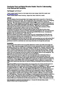
Saligny et al. Models for territorial dynamic studies Fig. 1: Canvases with 50 (in pink) and 25 km (in red) grid applied to the Seine Valley study area (M. Gabillot). The points represent axes from Middle Bronze Age. Map: K. Zaksek

In many mapping projects, a map is made out of the point samples collected in the field and then used to make predictions. To be consistent, every mapping project should have approximately an equal density of samples per area, also called inspection density. It is obvious that the denser the observation points the larger the scale of mapping. A cartographic rule, used for example in soil mapping, is that there should be at least one (ideally four) observation per 1  cm2 of the map. This principle can be used to estimate the effective scale of a data set consisting of sampled points only. For example, 10 observations per km2 correspond to the scale of about 1:50,000. The same principle can be also expressed mathematically A A SN = 100 ⋅ N … N [1] where SN is the scale number, A is the surface of the study area in m2 and N is the total number of observations. From cartographic rules the scale number can be used to estimate the grid resolution. If we take the intermediate number of 2.5 observations per cm2 and combine it with the pixel size p = 0.5 mm on the map rule of thumb, with a bit of reduction, we finally get a simple formula SN = 100 ⋅ 4 ⋅

A N [3] The following equations should therefore be used to choose the right pixel size for mapping point objects with known inspection density (for argumentations see Hengl 2006). p≈

Partners of the ArchaeDyn have agreed that a grid system designed in a vector model would be preferable, but planned in a way

to be easily converted to a raster model. This is important because archaeological data typically holds several attributes and storing such information in a raster model requires excessive storage. The raster model on the other hand offers good computation capabilities with map algebra. To facilitate conversion between the models we have decided to construct grids (canvases) consisting of squares in a predefined Lambert conformal conic projection. First the analysis grid size has to be defined for each individual study area. The proposed optimal cell size calculation is based on the assumption that data is approximately evenly distributed, which means that each data object is assigned the same area, defined by the cell. The cell size is therefore “unique” for each study area because it is directly related to the area of investigation and the number of observations – in effect it is an average distance among observations (Sánchez 2006). This empirical method is based on the assumption that if the objects are normally distributed, then a similar area should approximately belong to every object. Therefore, the average area of an object can be computed by dividing the whole area of interest by the number of objects. This average area is square shaped when working with a regular grid, thus the cell size of the grid can be computed by square rooting the average area. This number is then rounded and represents the optimal resolution [3]. p = 0.0791 ⋅

A N [2]

A similar approach is mentioned by Shary et al. (2002), but is contrasted to the finding of Hengl’s work, mentioned previously, by Colloque ArchæDyn – Dijon, 23-25 june 2008

27

Saligny et al. Models for territorial dynamic studies

approximately factor 10. This is due to the fact Hengl used different factors because of the tendency to map all the individual objects. Archaeological data is rarely evenly distributed, so in order to improve the statistical significance and aggregate the data we have calculated the optimal cell size and then chosen the first larger cell size, fitting the “standard” resolution system used in ArchaeDyn, i.e. 1, 2.5, 5, 10, 25, 50, 100, 250 km … This produces grids that are both optimal and well populated that is containing a significant number of points. In order to simplify the process of data transformations and comparison of different datasets further, the common point of origin has been defined for all the grids, meaning the cell boundaries of different resolutions and study areas overlap at the same coordinates. This means that even different scale phenomena can be processed as imagery in order to combine their information over the same or different areas when it is relevant. In the frame of the project we used a common projection, and a common origin point. The following projection has been used: • Projection: Lambert Conformal Conic • False Easting: 0 • False Northing: 0 • Central Meridian: 10 • Standard Parallel 1: 43 • Standard Parallel 2: 62 • Latitude Of Origin: 30 • Linear Unit: Meter All canvases are in vector format, enabling analysis in vector format and transformation to raster. Even though the canvases use different grid resolutions and are of different sizes, their cells overlap at the same coordinates, because they use the same point of origin (located approximately 500 km northwest of Ireland). Grid resolutions are scale dependent and are of factor 2, with some exceptions, values 100 m, 250 m, 500 m, 1 km, 2.5 km, 5 km, 10 km, 25 km, 50 km were mostly used.

3.3 From datation to temporal issues To study the territories is a question of space but to study their dynamics i.e. their trajectory and the transformation of their properties it is also a question of time. Time can be considered, similar as space, at different scales according to the phenomenon or the type of observation considered. Each type of observation has a scale within its own time framework. Therefore, it will be impossible to analyze at the same scale an inhabitat

28

Colloque ArchæDyn – Dijon, 23-25 june 2008

whose life is relatively short and territory whose persistence is generally much longer. In addition, the pace of changes that will affect the inhabitat will be much faster than mutations recorded by the territory. The team had to deal with a very strong contradiction: to understand the dynamics of territories over the long term using archaeological observations with extremely variable temporalities. To understand the phenomena of occupation / abandonment of the areas, concentration / dispersion of activities and to estimate the long-term degree of stability / instability of land managment, we should be able, according to the same repository, to compare phenomena revealed by the spatio-temporal distribution of several types of archaeological evidences. Because the chronological periods and the studied duration are different depending on each topic and each type of archaeological observation, the chronological development or the time scale which is a continuous phenomenon must be transformed into a discrete data similarly as it was done for space. This means a discretization of time with a regular or irregular unit, which can be different in each workgroup and study area. The time unit can be half-century, century, half-millennium, and millennium. Therefore the concept of temporal resolution was used to compare, in the same unit, the intensity of observed occupation. A common methodology was limited and the definition of the resolution was defined by each workgroup, sometimes by a simple choice. Within the framework of the workgroup 2, for example, a century unit was adopted and the settlements poorly dated were removed for the time series analysis, either directly either by reducing the geographical area of the initial corpus in order to keep the most reliable and accurate data (Bertoncello et al. 2008). To process the manuring unit whose datation is much more blurred, the team has adopted a broader resolution and a system included overlied bounds (Poirier et al. 2008). Finally, it was for the workgroup 3 that the problem has been most difficult to resolve, because the chronology is chrono-cultural based linked to each type of archaeological object being studied. In the project some methodological choices, that allow comparing databases between themselves and make possible the building of a repository with chronological bounds that can be easily used to analyze all data in a chronological continuum over the longterm (Neolithic to the modern period)were defined. The applied solution is similar as

Saligny et al. Models for territorial dynamic studies

for spatial approach, with a zoning whose boundaries are sometimes uncertain or unclear or whose boundaries are located between two limits of the cell of the adopted grid. In this case two solutions are usually adopted: 1) considering the continuous property of space, it is possible to take into account the values of the neighbourhood using a moving window to smooth the trend and avoid artificial breaks 2) the uncertainty or the fuzzy zone can be estimated, considering not the presence or absence, but a probability of existence. According to both principles, we decided 1) to work on mobile chronological bounds and 2) take into account the uncertainty of chronological bounds as a percentage that could be 25/50/75% (cf. Gauthier et al. 2008). The methodological choices defined by the three workgroups make possible the understanding of the results on a single chronological repository. This repository includes various resolutions depending on the studied phenomenon and the type of data. Even with various periods, it is possible to compare the trajectory of one or several areas according to the same chronological scale, just as it is possible to compare the spatial configurations from different areas of study or covering different periods. The protocol adopted by the team in order to deal with time and space issues is certainly arguable. Nevertheless, it provides a common framework to compare spatiotemporal distributions according to the scale of the studied data. In addition, it is a transparent framework which allows at each step of the analysis to return precisely the chronological and spatial scale of an observed phenomenon. Therefore, it gives a better understanding of the effects of scale that can impact the dynamics of the territories. The well defined common repository, chronological and spatial, change the way of our reasoning. The archaeological objects (or rather the “sum” of n object), initially described with a datation and a geographical location, are becoming an attribute of a part of area in a specified time. Such methodological position needs a strong consideration about the reliability of the databases and the data distribution.

2. Evaluation of databases and an measure of their reliability for analyses – confidence maps Inventory data used in archaeology are often incomplete and heterogeneous, making their interpretation, dating and localization a difficult task. They represent in fact a sample of a more complex reality. The analysis of archaeological data using spatial analysis tools therefore requires great caution in the interpretation that is drawn from them. The issue is to avoid the identification of spatial trends that are just a consequence of the degree of archaeological investigation. Otherwise, it is likely that the phenomenon described or estimated by any analysis is only a product of the method of inventory research (bibliography, prospecting…) and the level of investment used for the acquisition of the data. The objective was to develop a method for estimating an inventory for purposes of spatial analysis. This method has resulted in a tool whose product is the creation of a new layer of information: the map of confidence. This layer is generated by the combination of information reliability and performance. This tool, which has been described in more detail in Ostir et al. (2007), is briefly described below.

1.1 Representation maps Evidence for data dispersion/location over separate study areas is symbolized with representation maps. They were designed with the aim of being standardised in respect to the theoretical mean of the individual study area (i.e. variations to the average). Therefore they allow the quantification and visualization of spatial heterogeneity in the sampling and the inventory of the different datasets. The number of archaeological items in each pre-defined grid cell is computed and this value is compared to the expected (usually mean) value in the study area, which gives an idea of the over- or underrepresentation of data. Representation classes were defined to stand for: • no data, • normal representation, • over representation and • extreme representation. It was found that these types of classes correspond to the nature of archaeological data, whose frequency is typically exponentially distributed and hardly ever Colloque ArchæDyn – Dijon, 23-25 june 2008

29

Saligny et al. Models for territorial dynamic studies Fig. 2: A representation map of dated archaeological bronze objects in France (map: Z. Kokalj, data: F. Pennors).

normal. In case of being so, the classes would be under, normal, and over representation (fig. 2). Even though the process was designed with the aim of being non subjective and based solemnly on statistics, a uniform automatic statistical division of classes based on average proved to be unreasonable because of the extreme data heterogeneity, including different distributions, differences in absolute values, no data phenomenon, and the use of integer values. According to our tests, the classification process has to be done (semi)manually and individually for every dataset with the help of statistical and mathematical tools. The usual procedure is based on histogram analysis and its modification using a logarithmic function, and defining the natural breaks in the data. The latter are especially difficult to define if absolute frequencies (representations) are low. This implies the importance of selecting the optimal grid size. Too big cells result in overgeneralization, while too small grid cell sizes result in spatial discontinuity (in the extreme case one sample is represented wit one cell).

1.2

Reliability maps

Reliability maps express the settings (and limitations) of inventory exploration (i.e. how the archaeological sources were explored) in terms of common indicators such as survey level – sampling, visibility level, the

30

Colloque ArchæDyn – Dijon, 23-25 june 2008

quality of references etc., about a specific dataset. A reliability map gives information on the intensity of research and exploration (reliability of the inventory), and is not primarily concerned with the quality of data’s location. It can therefore also be interpreted as a correlation between intensity of research and actually identified sites or archaeological evidence. In our case a reliability map covers the entire study area and distinguishes three reliability levels (they are fully defined in the publications of ArchaeDyn workgroups, Ostir et al. 2007, Gauthier et al. 2008, Bertoncello et al. 2008): • high – reliable, • moderate – fairly reliable and • low – not reliable. It has been defined by the providers of individual datasets and has been mostly drawn by hand according to a predefined set of rules. The rules were defined by each workgroup or even by each archaeological team. Indeed, such rules are depending on the kind of investigation. Nonetheless, each set of rules is written with respect to the three predefined degrees allowing comparison. The definition of reliability levels is adjusted according to the nature of data. For example, instead of field walking, data availability in museums or publications can be considered. The identification of individual levels is based on an empirical method because its foundation is the knowledge on data, and is therefore inherently biased. It is also highly

Saligny et al. Models for territorial dynamic studies FIG3 Fig. 3: A reliability map of dated archaeological bronze objects in France (map: Ž. Kokalj, reliability zones and data: F. Pennors)

dependent on the phase of studies and of course directly connected to the state of the studied database.

1.3

Confidence maps

To represent the level of trust of the spatial analysis and modelling results we have defined a tool called confidence maps. Confidence maps provide the user a spatial impression about the representation and the reliability of the input data in the same time, giving him the opportunity to detect “artefacts”in the data.The same methodology has been defined for different scales and for different observed phenomena. Despite the fact that the data used can be very dissimilar the interpretation of confidence maps is the same. This is an innovation especially considering the extent of the ArchaeDyn project. Confidence maps offer a tool to evaluate the relevance of archaeological data in spatial analysis. They give an impression about the confidence a user can have on the final results that is based on input data. The representation and reliability layers are combined using map algebra (Tomlin 1990) in order to obtain confidence maps. The logic behind lies in joining two spaces: location-based density (representation) and intensity on inventory (reliability). Results allow for the comparison and analysis of data confidence and thus the evaluation of

the trustworthiness of the interpretation and spatial modelling, but also give information on the correlation between data representation and reliability. The map can be used to eliminate “spurious” zones for spacetime analysis over long-term (according to the comparison of each study area with their chronology and the interpretation key of the representation map). The proposed process is essentially based on simple algebraic operations and “binary” logic. The confidence was coded into two digit numbers, with one digit reserved for representation and the other for reliability. To technically enable the addition, the representation map has to have “denary” classes, 10, 20, 30, and 40, being extreme representation, over representation, normal representation and no data, respectively, and the reliability map was used with values of 1, 2, and 3, ranging from high, moderate to low reliability. The ensuing confidence map is in effect an overlay of both maps. By inspecting the map one can immediately find areas of different representation but also areas with different data reliability. The strongly coloured areas are more reliable than the light coloured areas but both can and should be included in the analyses with a different level of caution. The proposed process can also be applied to analyse and compare other spatial phenomena, and tests are underway to evaluate it for the effectiveness in representing temporal changes. Colloque ArchæDyn – Dijon, 23-25 june 2008

31

Saligny et al. Models for territorial dynamic studies FIG4 Fig. 4: A Confidence map of dated archaeological bronze objects in France (map: Z. Kokalj, data: F. Pennors).

There are still some problems that have to be solved. Confidence maps are not suitable for all databases. They suit better databases containing “noise” – they perform better with large amount of statistically well represented data. We have also found a rather strong scale dependence of the results. Different tests have shown that the tool performs better with small scale (big area), large quantity of points (often it will be studies of objects and not sites or settlements), and a low positional accuracy (studies about the diffusion of material, circulation of artefacts).

3. Developing the indices of spatio-temporal dynamics 3.1 Estimating the mean trends of mobility. 3.1.1 Common methodological principles In order to apprehend the spatial diffusions and dynamics over the long term, the three workgroups have each used the method of the barycentre or mean center, in spite of their different objects of study. This method belongs to the field of descriptive spatial statistics. The principle of the mean center (or barymetre or centre of gravity) consists in summarising a seed point by calculating the geographical mean of the spatial entities studied (Zaninetti 2005), which can eventually be weighted. The

32

Colloque ArchæDyn – Dijon, 23-25 june 2008

centre of gravity is then “a useful reference for comparing several seed points in a same geographical area or even for comparing the position of the same seed points over time” (Pumain and Saint-Julien 2001). Moreover, this method has already been used to this purpose in archaeology (Hodder and Orton 1976; Gauthier 2004 2005; Mordant et al. 2007). After having summarized the available information on a single point, the second aspect of descriptive spatial analysis consists in measuring the dispersion of the values around this index of central tendency, as the standard deviation shows the dispersion of values around a mean. The standard deviation ellipse is used to measure the dispersion of the values around the mean center of each phase. The standard ellipse takes into account the anisotropy of the distribution, in other words, its deformation in one direction or another (Zaninetti 2005). The long axis of the ellipse indicates the direction of the greatest variability between the values. Naturally, the direction of this ellipse can be influenced by the very pattern of the study area. In the Berry – Sancergues study area (fig. 5) for example, the stretching of the systematic surveying transect, orientated east-west, strongly conditions the direction of the ellipses which are calculated. In order to compare the spatial dynamics in the different micro-regions, it was necessary to normalize the measurements of the mean center’s displacements and the variations in the size of the ellipses in proportion to

Saligny et al. Models for territorial dynamic studies Fig. 5: Study of agrarian manuring –BerrySancergues study area: Mean center and dispersion (Sources and map: N. Poirier)

the common sizes. Thus in workgroup 1, the measurement of displacement of the mean centers for agrarian manuring was related to the greatest possible distance within the study area (larger diagonal), hence these displacements can be expressed in percentages. Another standardization was adopted by workgroup 2 for comparing the displacements of the mean center of settlement pattern systems in Languedoc and Limagne: the displacements measured between each step of time was related to the total sum of the displacements observed among all of the chronologies studied. In each of the workgroups, the variations in the size of the standard deviation ellipses from one phase to another were the object of a simple rate of variation (t = ((Va – Vd) / Vd) * 100 where Va is the end value (or size) and Vd is the start value (or size)). This standardization of measurements makes it possible to visualize on a single graph the variations of two chosen indices within different study areas. 3.1.2 The implementation particular to each workgroup In the context of the workgroup “Catchment areas”, the calculation of the mean center and the standard deviation ellipse were used with the goal of measuring the extent of the spatio-temporal dynamics which affect the localization of the cultivated areas over time, and to model the displacements and the dispersion of agrarian areas at each step in

time. This application to agrarian manuring was developed in the framework of a thesis (Poirier 2007). The calculated mean center is the center of gravity of a cloud of points formed by all of the centroids of the collection units of off-site artefacts at different periods. The localization of the seed point remains, of course, unchanged from one phase to another; what changes is the weighting of each of the points according to the density of off-sites artefacts collected in each area for each phase under consideration. The mean center is thus drawn towards the collection units which supplied the highest densities of off-site artefacts, those that are interpreted as having been the most intensely exploited during the chronological phase under study. A different mean center corresponds to each step in time (or chronological phase); each mean center is associated with a standard deviation ellipse whose size and orientation are also different. The measurement of the surface taken by each ellipse, and the observation of the variations in size of this ellipse from one phase to another can be interpreted as an index of the extension or the contraction of the intensely exploited areas. In practical terms, the more the ellipse is large and dilated, the more the spatial and quantitative variability of the manurings is important; on the contrary, an ellipse of a small size and restricted around the mean center is proof of the concentration of cultivated areas.

Colloque ArchæDyn – Dijon, 23-25 june 2008

33

Saligny et al. Models for territorial dynamic studies Hierarchical level Class1: agricultural buildings, small farms or small hamlets Class2: agricultural buildings, small farms or small hamlets Class3: farms or hamlets

Weight attributed 15 25 35

Class4: large farms or villages

45

Class6: agglomerations, large oppida Class7: atypical settlements

65

Class5: villae or villages/oppida

55

30

Tab.  1 Weight attributed to each hierarchical level

The period by period comparison of these two indices shows the spatial evolution of settlement patterns in a synthetic manner. Workgroup 3, which is focused on the raw materials and finished products from the Neolithic to the Bronze Age, has also used the mean center to summarize the seed points of archaeological discoveries.

Fig. 6: Displacements of mass metal mean centres during Bronze Age in Eastern France (Gauthier 2005a, Gauthier 2005b).

In the workgroup dealing with “Settlement patterns”, these two indices are a useful reference for comparing several seed points over time while measuring the stability of the settlement patterns. By using these two indices, we aim at identifying the phases of extension or withdrawal and pinpointing the variations in the localization of the occupied areas. The method was tested on two study areas, Languedoc and Limagne, and the calculations concerned the settlements occupied between the 5th c BC and the 7th c AD. Thus, for each chronological period, the mean center then corresponds to the mean of the coordinates X and Y of the settlements, weighted by the hierarchical level of the settlements. Effectively, since the variations in the number of occupied sites do not have the same significance depending on the nature and the function of the settlements, weight was attributed to each settlement in function of its hierarchical level (such as it had been defined by the automatic classification); this weighting was determined empirically after several tests (tab. 1).

34

Colloque ArchæDyn – Dijon, 23-25 june 2008

The described method was used with several aims in mind. The first concerns the comparison with the central point of the study area. The way in which the archaeological discoveries were spatialized determines the choice of this reference point. If their exact coordinates were used, we will choose the geometric centre of the area. If, however, the archaeological entities were spatizalized to the communal centroids, the mean center of the latter must be used as the centre of reference. Effectively, given that the communes do not have the same surface and that some regions present concentrations of communes of small size while other areas are made up of large communal territories, the entire study area does not have the same chance of receiving points. In the case of a well-balanced distribution, the mean center of the seed under consideration must remain close to the centre of gravity of the communes. An important deviation in relation to this reference point will show the presence of a large quantity of objects which “pull” the mean center in its direction. The orientation of the vector linking the centre of reference and the mean center shows the general direction taken by all of the distributions. Its length indicates the importance of the variation in comparison to a random distribution. Another objective was to compare several distributions in the framework of the process of the diffusion of a phenomenon over time, such as the circulation of types of objects (Pumain and Saint-Julien 2001). In order to understand the impact of the chronological evolutions, we can then plot the vectors linking the successive phases

Saligny et al. Models for territorial dynamic studies

so as to show the progression of the mean centers. The orientation of the vectors shows the direction of the changes. Their length indicates the extent of the variation: if the displacement made is important or if it remains low. Depending on the case, the calculation of the geographical mean of each area was weighted with quantitative information (number of objects, mass of the object, etc.) which was judged to be useful for interpreting the spatial and chronological evolution of the phenomenon shown. Finally, the mean center was exploited in this group in order to compare the relative position of the typological sets as well as the positions of the mean centers of different materials with their respective mineral deposits (fig. 6). 3.1.3 Critical feedback and possible avenues of development It is interesting to note that, in spite of their different objects of study and working with very variable scales of time and space (from the temporal resolution of a half a century to that of a millennium,and from the community land to the European continent), the three workgroups had recourse to the same indices of spatial statistics. This methodological convergence is necessarily accompanied by important differences in implementing, in particular, the choice of the variables used to weight the archaeological variables used in the analysis. Thus the workgroup focused on catchment areas is based on a purely quantitative weighting (the density of the shards of each chronological phase gathered in the collection units). As for the workgroups centred on settlement patterns, they implemented a weighting based on a qualitative evaluation (the organization of settlement hierarchies originating from the CAH) which was itself elaborated by using descriptors that can be either qualitative (the abundance of the materials) or quantitative (the surface of the settlement). Finally, the workgroup dealing with raw materials and finished products used the two types of weighting, quantitative when the evolution observed is based on the weight of the objects, qualitative when the distribution of Alpine axes in function of their typochronological membership or their degree of finish is analysed. For two of the three workgroups, out of concern for the comparability of situations observed in the different study areas under consideration, it was decided to use the relative measurements of the spatiotemporal processes shown, which can then be

expressed by evolutions in percentages. This opens up the way to cross the observations realized in each workgroup in the future continuation of the programme. It would be worthwhile, for example, to compare the dynamics of the settlement with that of associated agrarian areas: are the rhythms of evolution of the fabric of settlement patterns the same as those of cultivated areas? This ambition, however, is confronted by a certain number of difficulties linked in particular to the different resolutions of the processes observed: first, spatial resolutions which do not always make it possible to compare evolutions readable on a local scale and others on a continental scale; then temporal resolutions, determined in a large part by our capacities to date archaeological objects. Moreover, the two can be linked, insofar as the processes which are effective on a small spatial scale (European) can only be apprehended over the long term. In short, a comparison of the different scales of time and space according to the spatio-temporal processes studied will enable us to shed light on their complementarities as well as their contradictions.

3.2 Assessment of the degree of stability / instability for spaces 3.2.1 Density estimation To assess the degree of stability or instability spaces we have to observe changes taking place between two or more periods. From the original data that are punctual (discrete), we are already committed to produce a continuous surface. The development of this information is based on the assumption that each data recorded in precise location is really the point through a space in occupied area, crossing or even enhanced by a community whose archaeological object reflects the activity. There are several reasons for this “uncertainty”, including the sampling and localization method. Under these specific conditions it is assumed that the archaeological record represents a continuous occupation of space. It also considers that the concentration of objects / sites may be an indicator of intensity of the space occupied. Under these assumptions, the team has implemented two methods to restore the continuity of space 1) focal sums and 2) the method of kernels. The method of focal sums is a method of map algebra (Tomlin 1990) used to reconstitute the continuity of space (i.e. to fill the space in its entirety) without assuming continuity Colloque ArchæDyn – Dijon, 23-25 june 2008

35

Saligny et al. Models for territorial dynamic studies

the variation of the phenomenon studied, unlike interpolations. The methodology of focal sums has already been published in the archaeological context (Gauthier 2004 and 2005). Basically, in a grid each grid cell is assigned the sum of all cells belonging to a larger surface surrounds, called neighbourhood. So this is a density calculation which takes into account the immediate vicinity and that integrates and a larger “relations” space (concentrations, diffusions) between the cracks. It helps to restore the continuity of space without making interpolation on the data. This method has been used for the workshop 3 to highlight the main areas of concentration of spatial entities. The maps were produced for each area to present the main concentrations of archaeological discoveries and compare several parameters within the same corpus (type, material, types of sites…). The parameters used are always the same, so it is also possible to compare different corpus. Nevertheless, one should not directly compare the values in the grid, but rather the relative position of the main areas of concentration. It then looks at whether the main areas of consumption of various products are the same or whether different trends are emerging, reflecting differences in their modes of use or dissemination. One of the critical issues is the choice of grid cell size and the shape of the focus (square, circle). If the grid is too small regarding the sampling density the continuation of space is not ensured. The distance of the points taken into account around the central point in the “focus” is not always the same (for square focus the points placed at the corners far from the centre should not contribute the same as closer points). The values of cells located at the ends of the neighbourhood are provided to the cells close to the centre. According to the choice of starting grid and the size of the neighbourhood, this can then create effects of “false” concentrations in areas located between two areas of lower concentrations. Finally, on the study area, the neighbourhood taken into account with the method is is reduced to only cells in the study area; neighbourhoods are therefore not actually equal in size. This simple map algebra method has been extensively discussed in the workgroup 4 and the effects depending on the size of the neighbourhood; circular focus with the size that is close to the estimated sampling (point) density gives the best results. The problems however lead team to consider another method of calculation involving a kernel type function.

36

Colloque ArchæDyn – Dijon, 23-25 june 2008

Using mapping and the kernel density estimation method (KDE) several tests to produce continuous density surfaces in order to represent the distribution of archaeological entities have been performed. Like the focal sum, the KDE method provides an estimation of the density according to a moving window. The difference is in the density value calculation. Focal sum is working similar as a “naïve estimator” (see above), while with KDE the obtained density value takes into account the distance of the neighbourhood. From the centre of the window with the increasing distance the weight of the neighbourhood decreases in the density estimation according to the model chosen (the so called kernel function). The method is well known (Silverman 1978 and 1986, Wand and Jones 1995, Zaninetti 2005) and was already used for archaeological applications, in particular with statistical coordinates provided by principal component analysis or for intra-site analysis purpose (Baxter and Beardah 1997, Beardah 1999). The method is more traditionally used for geographical space by geographers (Grasland et al. 2000). The density estimation obtained using KDE is dependent on two main parameters: 1) k the kernel function chosen, 2) h the radius chosen. Because the KDE method was used as a part of an exploratory process we did not toughly test the individual parameters (this should be done later to ensure the robustness of the obtained results). Within a first step and from a practical point of view, we used the kernel function implemented in the ArcGIS. The kernel function used by ArcGIS is based on a quadratic kernel function (Silverman 1986) and there is no way to change it (a more open software should be used to provide “controlled” results). Nevertheless, based on the assumption that the result of the analysis is not strongly influenced by the kernel function as long as the function is symmetrical (Silverman 1978), for the moment no additional tests were made using different k. Mathematically an estimate of the density F(x) using a quadratic kernel function can be written as

For any grid cell j and point i of the observed distribution, F(xj) is an estimate of the density. The weight function W is used to ensure that the sum of new values is the same as the total sum at the observed values, while h is the radius, d is the distance between i and j; if dij> h then F(xj) = 0 otherwise F(xj) > 0.

Saligny et al. Models for territorial dynamic studies Fig. 7: Naïve estimator and quadratic kernel function.

xj

xj

xi

xi h

A- naive estimator

h

B- quadratic function L. Nuninger 2008

Fig. 8: Representation of the maximal density values according to h (radius). Highest values are giving too much importance to isolated points whereas lowest values provide almost no information. The optimal radius for density estimation corresponds to the inflection point.

The difference between the naïve estimator and the quadratic kernel function is shown in fig. 7. The choice of the radius h is very important (Silverman 1978) because h determines the degree of smoothing. Usually, large values of h over-smooth, while small values of h under-smooth the data and produce peaks around data clusters. There are many ways to define the optimal value of h, which can be fixed for the entire study area or adjustable. Within the Archaedyn project we used a fixed h but further tests has to be performed with adjustable h. Statistical indicators based on the data distribution can help to choice h (Baxter and Beardah 1997, Zaninetti 2005) but there is no explicit determination method and the user has to make an aribrary decision, based on criteria similar to the ones described for the grid cell size. In general, using too small radius will produce an irregular surface that is

problematic especially when the total number of point i is relatively small. On the contrary, too big radius will result in the lost precision in favour of general trends. Within the Archaedyn project we had to choose an optimal radius for different study areas in order to enabvle the comparison of results. Since the approach was fuzzy enough according to the site locations and because the purpose was to compare relative values over time based on general tendencies, a simple graphical way was used to define the optimal value of h (Fig. 8). According to this method, several radii were tested on several study areas in order to define the range of optimal values. KDE was then processed for each study area for several analyses (Gauthier et al. 2008, Bertoncello et al. 2008). In particular, the density estimation was used to evaluate changes over time and defined aggregates for qualitative analysis. Colloque ArchæDyn – Dijon, 23-25 june 2008

37

Saligny et al. Models for territorial dynamic studies

3.2.2 Mapping density changes To evaluate changes from period to period and to have an overview of the developing/ declining/stable areas, density maps processed according to the method described above were used. The basic idea was observe the serial arrangement of period or state (T0, T1, T2…) and to detect the dynamics between those states. To evaluate the difference between two maps a simple subtraction (T1 – T0) was used first. However, the method was not very acceptable since it was difficult to quantify a comparable difference between several areas. Therefore the so called “normalized ratio” which quantifies the ratio of two density value T1/T0 or the relative difference, for example (T1-T0/T0) (Béguin and Pumain 2003), were used. We can describe this in more detail with an example from the workgroup 2. In the first case, values close to 1 represent the stability of the occupation whereas values greater than 1 represent an increase of the settlement in the surrounding area (e.g. 0.33 down two-thirds, 0.5 decrease by half, 2 density doubled; 3 density multiplied by three). In the second case, the processing of the relative difference has the advantage of providing negative values for declining intensity, positive for the increase and a zero value for stability (no change), which makes the interpretation of results easier. Several formulas can be used to process the relative difference, two of them were studied: 1. (T1 - T0) / T0, where -0.66 means down by two thirds, -0.5 drop by half, 1 density doubled, 2 increase by two thirds. This method has the advantage of being easily readable when the density decreases, while the increase in density will be less easy than for the simple ratio T1/T0. 2. (T0 - T1) / (T1 + T0), which is a normalized differential ratio (e.g. -0.33 down by half, 0.33 double strength; -0.5 down twothirds, 0.5 increase three times). In addition it provides a useful tool to easily compare the values of changes resulting from an increase or a decrease of the occupation. The normalized differential ratio was therefore mainly used for the analysis (Bertoncello et al. 2008).

3.3 From hierarchical typology to the spatial structuring index or level of hierarchical organization The experiment performed by workgroup 2 aims to introduce the results of the qualitative analysis of settlement in the process of the density estimation. The approach has two goals: 1) to weight the quantitative data (number of settlement) using a qualitative variable, and 2) to define areas according to their level of structuring. In order to understand the settlement organisation over the long term, a hierarchical typology was done using a factor analysis (AFC) and an agglomerative hierarchical clustering (CAH) from the AFC results. Both analyses provide a classification of the settlement (Bertoncello et al. 2008). The values defined for each ordered class or extracted from the first axes of the AFC for each settlement were used to weight the density estimation. Under this condition, it was estimated that small settlement provide a low density power whereas high hierarchical settlement can be account as many small settlements. The method was tested on the 11 study areas but the interpretation has to be systematically done in order to validate the process and its interest. The second qualitative approach is probably the most interesting. The density maps are able to distinguish sectors or areas with different level of occupation during certain periods of time. In addition, we wanted to observe the differences between these sectors according to different types of settlement that have occupied. Two indicators were calculated to determine the spatial structuring of the settlement i.e. the level of hierarchical organization of settlement within each sector: 1) The hierarchical variety of the settlement which shows the degree of diversification of the settlement types (see above and Bertoncello et al. 2008). 2) The differentiation of the present class in each sector. For an equivalent value of the variety, we can distinguish: a) a low range - i.e. a high homogeneity - which indicates the association of settlements belonging to classes of close hierarchically (e.g. classes 1 and 2, or classes 5 and 6), b) a high range or a strong differentiation when classes are extreme (e.g. classes 1 and 6). This synthetic analysis, carried out on periods of four centuries (Bertoncello et al. 2008), enables the differentiation of areas according to the general tendencies of the settlement

38

Colloque ArchæDyn – Dijon, 23-25 june 2008

Saligny et al. Models for territorial dynamic studies

settlement density (radius of 1000m)

inputs

Fig. 9: Processing model of the spatial structuring index

settlements

Reclassification

reclassified density (quantile classification) Conversion to vector format

reclassified density

Definition of areas of analysis (aggregate of settlements)

Manual cutting

AREA

Zonal statistics

settlements

- variety - standard deviation

Spatial join

Showing spatial structure (calculation of indicators)

AREA 1

output

AREA 1 standard deviation

AREA 1 variety

Combining mapping

vector file

raster file

texte file

Fig. 10: Definition of the sectors based on settlement aggregates

a

b

organization: low level of organization (little diversified and differentiated), average and high level of organization (diversified and showing a large spectrum of types of settlements). It can also take into account associations and differences between neighbouring settlements without focusing on the value of classes that are poorly represented for some of them in certain regions. From a methodological point of view, the approach is divided into several stages (fig. 9). In the first part the areas of analysis are defined. Several tests were made with grid, with focal sum method and finally with a density estimation using the KDE method. The first two solutions have been abandoned because the cells were too large grouping together settlement geographically too far away and because the naïve estimator created artificial areas of concentration among sites location. Finally, using the KDE method with a quadratic function and a fixed radius (1000 m), several areas were defined. In this case a simple density

c

d

was used (without any weight according to hierarchical classification). The scale of observation aggregates settlements based on the normal distribution of in each study area. The aggregates have been identified manually by visual analysis for each of four periods under consideration (Fig. 10). The second step corresponds to the processing of both indicators, i.e. variety and range. Within each sector the value of the variety is the number of different classes. The few settlements poorly informed that have therefore not been taken into count in the classification, contribute to the calculation of sectors, but are not involved in calculating the variety (Bertoncello et al. 2008). The index of range is obtained by calculating the standard deviation between the classes located within the sector under consideration (coded from 1 to 6). The settlement from the class 7 were not used, since they group atypical settlements (see above and Bertoncello et al. 2008), and an association with settlements from class 6 e.g. does not mean a low level of differentiation.

a. settlement distribution (with a buffer) b. settlement density estimation (based on the number only) c. definition of the aggregates or area (sector) of analysis d. sectors and settlements according to their hierarchical class

Colloque ArchæDyn – Dijon, 23-25 june 2008

39

Saligny et al. Models for territorial dynamic studies Fig. 11: Levels of variety and range

Fig. 12: Different combinations of the indices of hierarchical variety and range which show different levels of hierarchical organization of the settlement patterns

The last step considers the combination of both indicators in order to define the index of structuring or level of hierarchical organization. A simple combination was used in this study since both indicators (variety and range) are correlated – if the number of classes is high it is very probably that the range is high giving a high importance. Degrees of variety and range are therefore distributed to three levels: low, medium and high (Fig. 11). The three levels of range were defined using theoretical examples which are representing associations of more or less homogeneous settlements i.e. with a degree of diversification relatively low (tab. 2) Number of present classes 2 3 4 5 6

Theoretic combination

Standard deviation

1&2 1&6 1, 2 & 3 1, 3 & 6 1, 2, 3 & 4 1, 3, 5 & 6 1, 2, 3, 4 & 5 1, 3, 4, 5 & 6 1, 2, 3, 4, 5 & 6

0.81 2.5 0.81 2.05 1.11 1.92 1.41 1.72 1.70

Tab. 2: Definition of the levels of range

The graphical combination of both variables indicates the degree of the settlement organization inside a sector. It makes possible the distinction, in diagonal, between sectors poorly structured (non-diversified settlement types with similar hierarchical level) and sectors highly structured (strongly diversified and presenting a broad spectrum of settlement classes). In horizontal, for

40

Colloque ArchæDyn – Dijon, 23-25 june 2008

a similar degree of variety, it is possible to distinguish the tendency towards differentiation between classes. Thus, a low range associated with a high level of differentiation will highlight an area whose settlement pattern is highly hierarchical but according to a level of structuring fairly simple. In vertical, for a similar level of differentiation, it will highlight a tendency towards homogeneity of the settlement system. Despite a variety that can be high, the lowest level of differentiation shows a complex system of organization but weakly organized into a hierarchy. From this point of view, the settlement pattern is considered as homogeneous. When effects of a high variety and a high level of differentiation are cumulated then a high level of structuring or hierarchical organization illustrating a complex settlement pattern strongly organized into a hierarchy it reached. The approach developed to analyse the level of hierarchical organization of settlement is still experimental and has been tested on a single study area (Eastern Languedoc) only. The method should be improved in many aspects. There are problems remaining with unclassified or atypical settlements, for example. Furthermore, the result is to a great extent dependent on the identified aggregates or sectors used for the analysis. The adopted solution to define the aggregates of settlements (see above) is not really satisfactory and is too subjective. We will improve certain steps of the model and in parallel, the method has to be tested on other study areas where settlement densities are different (e.g. Argens-Maures).

Saligny et al. Models for territorial dynamic studies

Conclusion Thanks to the contribution of a large team, according to the scientific richness of the archaeological corpus and because of ambitious thematic issues, the ArchaeDyn program provides a good framework to develop tools and methods for spatial analysis in archaeology. The workgroup 4 – Tools and methods of spatial analysis – has successfully linked experts from other thematic workgroups as well as from outside of the program and has helped to develop many exploratory analyses methods to develop a common protocol that will enable comparison between different corpus, regions or time periods. From this point of view, the confidence map tool is unprecedented progress, at least in the French archaeological community. Spatial analyses developed by the Archaedyn’s team are significantly advanced regarding

those of the Archaeomedes programs (Favory and Nuninger 2008b). The analysis of time dynamics has not been completed to reach the initial ambitious, however. In most analyses, time is omnipresent but as a series of “time” shots. The analysis of the trajectories and maps of changes all include a time dimension and provide a representation of the results; the analysis of the process itself has not been reached. In addition, the program was too short to thoroughly study each method used, to apply all analyses to all study areas, and carry out an extensive interpretation of the results. Such interpretations are now needed to refine and validate the analysis models. The methodological development has been very dynamic but it is far from concluded. In a later stage, the team plans to consolidate its first approaches in order to implement them systematically and in parallel to develop new exploratory fields particularly on the analysis of spatial dynamics itself.

Colloque ArchæDyn – Dijon, 23-25 june 2008

41

Saligny et al. Models for territorial dynamic studies

Bibliography Baxter et al. 1997 Baxter M.J., Beardah C.C., Wright R.V.S. – Some archaeological applications of kernel density estimates. Journal of Archaeological Science, 24, 347-354. Beardah 1999 Beardah, C. – Uses of multivariate kernel density estimates. In: Dingwall, L., Exon, S., Gaffney, C. F., Laflin, S., and van Leusen, M., eds., Archaeology in the Age of the Internet: Computer Applications and Quantitative Methods in Archaeology 1997, volume S750 of BAR International Series. Archaeopress, Oxford. Béguin and Pumain 2001 Béguin M., Pumain D. – La représentation des données géographiques, statistique et cartographie, Paris, A. Colin (coll. cursus). Bertoncello 1999 Bertoncello F. – Le Peuplement de la basse vallée de l’Argens et de ses marges (Var, France), de la fin de l’Age du Fer à la fin de l’Antiquité. Thèse de Doctorat, Aix-en-Provence, Université de Provence. Bertoncello 2002 Bertoncello F. – Villa/vicus: de la forme de l’habitat aux réseaux de peuplement. In: Garmy (P.), Leveau (Ph.) éd.  – Dossier Villa et vicus en Gaule Narbonnaise. Revue Archéologique de Narbonnaise, 35: 39-58. Bertoncello and Gandini 2005 Bertoncello F., Gandini C. – Valeur et pertinence des indicateurs hiérarchiques de l’habitat rural antique: quelques réflexions à partir des établissements berrichons. In: Berger (J.-F.), Bertoncello (F.), Braemer (F.), Davtian (G.), Gazenbeek (M.) – Temps et Espaces de l’Homme en Société: Analyses et modèles spatiaux en archéologie. Actes des XXVe Rencontres Internationales d’Archéologie et d’Histoire d’Antibes, 21 – 23 octobre 2004. Valbonne, Éditions APDCA: 237−248. Bertoncello et al. 2008 Bertoncello F., Fovet E., Gandini C., Trément F., Nuninger L. with the collaboration of the WG2’s team. – The spatiotemporal dynamic of settlement pattern from 800 B.C. to 800 A.D. in central and meridional Gaul: models for an inter-regional comparison on the long term.in 7 millennia of territorial dynamics: settlement pattern, production and trades, from Neolithic to Middle Ages, pre-proceedings of the Archaedyn 2008 conference, Dijon 23-25 June. Bishop et al. 2001 Bishop T.F.A., McBratney A.B., Whelan B.M. – Measuring the quality of digital soil maps using information criteria. Geoderma 103 (1): 95–111. Durand-Dastès et al. 1998 Durand-Dastès F., Favory F., Fiches J.-L., Mathian H., Pumain D., Raynaud C., Sanders L., Van der Leeuw S. – Des oppida aux métropoles: Archéologues et géographes en vallée du Rhône. Paris, Economica, 275 p.

42

Colloque ArchæDyn – Dijon, 23-25 june 2008

ESRI 2006 ESRI – Cell size. ArcGIS desktop help documentation. ESRI Inc., Redlands, CA. Fotheringham et al. 2000 Fotheringham A.S., Brunsdon C., Charlton M.E. – Quantitative Geography, Sage, London. Favory et al. 1987-1988 Favory F., Fiches J.-L., Girardot J.-J. – L’analyse des données appliquée à la typologie des sites gallo-romains dans le Beaucairois (Gard): matériel de prospection et environnement paysager. Essai méthodologique. Gallia, 45: 67-85. Favory et al. 1994 Favory F., Girardot J.-J., Raynaud C., Roger K. – L’habitat gallo-romain autour de l’Étang de l’Or (Hérault): hiérarchie, dynamique et réseaux du IIème s. av. au Vème s. ap. J.-C. In: Mactoux M.-M., Geny E. éd. – Religion, anthropologie et société. Paris, Annales Littéraires de l’Université de Besançon: 123-215 (Mélanges Pierre Lévèque, 8). Favory et al. 1998 Favory F., Van der Leeuw S. – Archaeomedes, la dynamique spatio-temporelle de l’habitat antique dans la vallée du Rhône: bilan et perspectives. Revue Archéologique de Narbonnaise, 31: 257-298. Favory et al. 1999 Favory F., Girardot J.-J., Nuninger L., Tourneux F.-P. – Archaeomedes II: une étude de la dynamique de l’habitat rural en France méridionale, dans la longue durée (800 av. J.-C. – 1600 ap. J.-C.). AGER, 9: 15-35. Fiches et al. 1987 Fiches J.-L., Gasco Y., Michelozzi A. – L’occupation des sols et l’exploitation de l’espace rural. In: Bessac J.-C., Christol M., Fiches J.-L., Gasco Y., Janon M., Michelozzi A., Raynaud C., Congès A. R., Terrer D. éd. – Ugernum: Beaucaire et le Beaucairois à l’époque romaine, I. Caveirac, ARALO: 85-112 (Cahiers de l’ARALO, 15). Gauthier 2004 Gauthier E. – L’évolution de la consommation du métal à l’Âge du Bronze, en France orientale et en Transdanubie. The Development of Metal Consumption in eastern France and the Transdanube during the Bronze Age, Histoire et Mesure, n° XIX-3/4, Systèmes d’Information Géographique, Archéologie et Histoire: 345-376. Gauthier 2005 Gauthier E. – La Consommation du métal en France orientale et en Transdanubie du XVIIè au IXè s. avant notre ère. Analyse spatiale et modélisation des systèmes socio-économiques de l’Age du Bronze, thèse de doctorat, Universités de Bourgogne et de Budapest, sous la direction des professeurs Claude Mordant et Miklós Szabó, inédite, 357 p., 134 pl., 39 tabl. et annexes.

Saligny et al. Models for territorial dynamic studies

Gauthier et al. 2008 Gauthier Es., Weller O., Nuninger L. with the collaboration of Gabillot M., Quilliec B., Petrequin P. – Models for the study of the consumption and the circulation of resources and products in France and Western Europe during the Neolithic and the Bronze Age (Programme ArchaeDyn). In 7 millennia of territorial dynamics : settlement pattern, production and trades, from Neolithic to Middle Ages, pre-proceedings of the ArchaeDyn 2008 conference, Dijon 23-25 June. Grasland et al. 2000 Grasland C., Mathian H., Vincent J.M. – Multiscalar Analysis and map generalisation of discrete social phenomena: Statistical problems and political consequences, Statistical Journal of the United Nations ECE, 17, IOS Press. Hengl 2006 Hengl T. – Finding the right pixel size, Computers & Geosciences, 32: 1283–1298. Hodder and Orton 1976 Hodder I., Orton C. – Spatial analysis in archaeology. Cambridge: Cambridge University Press, VIII-270 p. Mordant et al. 2007 Mordant C., Rottier S., Saligny L. – Dynamisme et espaces culturels. De la notion de mobilité au sein des populations, du Bronze moyen à l’étape initiale du Bronze final en France orientale (XV-XIIIe s. av. J.-C.), in H. Richard, M. Magny et C. Mordant, Environnements et cultures à l’Age du Bronze en Europe occidentale, actes du 129e CTHS, Besançon, Paris, ed. CTHS: 143-157. Nuninger 2002 Nuninger L. – Peuplement et territoires protohistoriques du VIIIe au Ier s. av. J.-C. en Languedoc oriental (GardHérault). Thèse de Doctorat, Université de Franche-Comté, Besançon. (http://tel.ccsd.cnrs.fr/documents/archives0/00/00/29/81/ index_fr.html) Nuninger et al. 2007 Nuninger L., Tourneux F. P., Favory F. – From Archaeomedes to Archaedyn. Layers of Perception. Proceedings of the 35th Computer Applications and Quantitative Methods in Archaeology Conference, Berlin, Germany, April 2-6, 2007 *(Kolloquien zur Vor- und Frühgeschichte, vol. 10). Bonn (Germany): Habelt. Nuninger and Favory 2008a Nuninger L., Favory F. – Introduction to the ArchaeDyn project - Spatial dynamic of settlement patterns and natural resources: toward a long-term integrated analysis from Prehistory to the Middle Ages. In 7 millennia of territorial dynamics  : settlement pattern, production and trades, from Neolithic to Middle Ages, pre-proceedings of the ArchaeDyn 2008 conference, Dijon 23-25 June.

Nuninger and Favory 2008b Nuninger L., Favory F. – ArchaeDyn 2005-2007: ambitions, achievements and accomplishments. In 7 millennia of territorial dynamics  : settlement pattern, production and trades, from Neolithic to Middle Ages, pre-proceedings of the ArchaeDyn 2008 conference, Dijon 23-25 June. Oštir et al. 2007 Oštir K., Kokalj Ž., Saligny L., Tolle F., Nuninger L. – Confidence maps: a tool to evaluate archaeological data’s relevance in spatial analysis, (with the collaboration of Françoise Pennors and Klemen Zaksek), Layers of Perception. Proceedings of the 35th Computer Applications and Quantitative Methods in Archaeology Conference, Berlin, Germany, April 2-6, 2007 *(Kolloquien zur Vor- und Frühgeschichte, vol. 10). Bonn (Germany): Habelt. Poirier 2007 Poirier N. – Un espace rural en Berry dans la longue durée: expérience de micro-analyse des dynamiques spatio-temporelles du paysage et du peuplement dans la région de Sancergues (Cher), Thèse de doctorat, Université François-Rabelais de Tours. (http://tel.archives-ouvertes.fr/tel-00212332/fr/) Poirier et al. 2008  Poirier N., Georges-Leroy M., Tolle F., Fovet E. – The time-space dynamics of agricultural areas from Antiquity to Modern Times in 7 millennia of territorial dynamics  : settlement pattern, production and trades, from Neolithic to Middle Ages, pre-proceedings of the ArchaeDyn 2008 conference, Dijon 23-25 June. Pumain and Saint-Julien 2001 Pumain D., Saint-Julien T. – Les interactions spatiales, Paris, A. Colin (coll. cursus), 189 p. Sánchez 2006 Sánchez, J., 2006. The accuracy of grid digital elevation models linearly constructed from scattered sample data, International Journal of Geographical Information Science 20 (2): 169-192. Sanders 1989 Sanders L. – L’analyse des données appliquée à la géographie. Alidade, RECLUS, Montpellier, 1989. Shary et al. 2002 Shary P., Sharaya L., Mitusov A. – Fundamental quantitative methods of land surface analysis, Geoderma, 107: 1-32. Silverman 1978 Silverman B.W. – Choosing a window when estimating a density, Biometrika, 65, p. 1-11. Silverman 1986 SILVERMAN B. – Density Estimation for Statistics and Data Analysis, London: Chapman and Hall.

Colloque ArchæDyn – Dijon, 23-25 june 2008

43

Saligny et al. Models for territorial dynamic studies

44

Stein et al. 2001 Stein A., Riley J., Halberg N. – Issues of scale for environmental indicators. Agriculture, Ecosystems & Environment 87 (2): 215–232.

Vieux and Needham 1993 Vieux B., Needham S. – Nonpoint-pollution model sensitivity to grid-cell size. Journal of Water Resources Planning and Management, 119 (2): 141–157.

Tomlin 1990 Tomlin, D.C. – Geographic information systems and cartographic modeling. Englewood Cliffs: 572 p.

Wand and Jones 1995 Wand M.P., Jones M.C. – Kernel Smoothing, Monographs on Statistics and Applied Probability, Chapman and Hall, 1995.

Van der Leeuw et al. 2003 Van der Leeuw S., Favory F., Fiches J.-L. (dir.) – Archéologie et systèmes socio-environnementaux: Études multiscalaires sur la vallée du Rhône dans le programme ARCHAEOMEDES. Paris, CNRS Éditions, (CRA Monographies, 27), 403 p.

Zaninetti 2005 Zaninetti J.-M. – Statistiques spatiales, méthodes et applications géomatiques, Lavoisier, Paris, 320 p.

Colloque ArchæDyn – Dijon, 23-25 june 2008