Modified Bayesian approach for the reconstruction of dynamical ...

PHYSICAL REVIEW E 73, 036211 共2006兲

Modified Bayesian approach for the reconstruction of dynamical systems from time series D. N. Mukhin,* A. M. Feigin, E. M. Loskutov,† and Ya. I. Molkov Institute of Applied Physics, Russian Academy of Sciences, Russia 共Received 5 May 2005; revised manuscript received 17 January 2006; published 16 March 2006兲 Some recent papers were concerned with applicability of the Bayesian 共statistical兲 approach to reconstruction of dynamic systems 共DS兲 from experimental data. A significant merit of the approach is its universality. But, being correct in terms of meeting conditions of the underlying theorem, the Bayesian approach to reconstruction of DS is hard to realize in the most interesting case of noisy chaotic time series 共TS兲. In this work we consider a modification of the Bayesian approach that can be used for reconstruction of DS from noisy TS. We demonstrate efficiency of the modified approach for solution of two types of problems: 共1兲 finding values of parameters of a known DS by noisy TS; 共2兲 classification of modes of behavior of such a DS by short TS with pronounced noise. DOI: 10.1103/PhysRevE.73.036211

PACS number共s兲: 05.45.Tp, 02.70.Rr, 02.30.Zz

I. STATISTICAL APPROACH TO RECONSTRUCTION OF DYNAMIC SYSTEMS

Reconstruction of DS from TS generated by this system is usually understood as seeking its evolution operator. When a DS is known, it is necessary to find values of parameters that determined evolution of the system during TS generation. Such a formulation of the problem arises, for instance, when chaotic regimes of DS behavior are used for solution of the problem of coded transmission of information 共see, e.g., Ref. 关1兴兲. In situations typical for most natural systems 共atmospheric-oceanic, tectonic, biological兲, the DS that generated the observed TS is unknown. In this case, reconstruction of DS means construction on the basis of the information contained in the TS of a parametrized model of unknown evolution operator. Apparently, such a model cannot be ideal as, generally, there does not exist such a set of parameter values for any class of models that would make the model absolutely adequate to the modeled DS. Inevitable discrepancy between them is called “defect of the model.” In this sense, the two above formulations of the problem of DS retrieval are sometimes classified as the “perfect model class scenario” and the “imperfect model class scenario” 关2兴. Assume that we have at our disposal the vector TS x, M and which is formed by M observed quantities x = 兵x共m兲其m=1 共k兲 d connected with DS state u = 兵u 其k=1 via an observer h, x = h共u兲. Here d is DS dimensionality, d 艌 M 艌 1. Under the perfect model class scenario d value is naturally known to us. When DS is unknown this quantity may be estimated by minimal embedding dimension of the attractor responsible for its observed evolution. Methods of obtaining this information and quite substantial restrictions were discussed by numerous authors and summarized in different review papers and books 共see, e.g., Refs. 关3,4兴兲. In this work we restrict our consideration to the first situation. The second situation 共the “imperfect model class scenario”兲 will be considered elsewhere.

*Electronic address: [email protected] †

Electronic address: [email protected]

1539-3755/2006/73共3兲/036211共7兲/$23.00

In what will follow we will use the following formulation of the Bayes theorem 关5兴. Suppose that the system under experiment possesses a set of properties 共parameters兲 ␮ that cannot be measured directly and let values of x be recorded in experiment. Then, posterior conditional probability density of unobservable parameters 共frequently referred to as likelihood兲 p共␮ 兩 x兲 is proportional to the product of their prior probability density p共␮兲 and prior conditional probability density of the obtained experimental results, p共x 兩 ␮兲: p共␮兩x兲 = C ⫻ p共␮兲 ⫻ p共x兩␮兲.

共1兲

It will be clear from what will follow that conditional probability density p共x 兩 ␮兲 depends wholly on the way TS becomes noisy and on probability densities of all noises present in the TS. Factor p共␮兲 takes into account a priori information about the system. If such information is not available, probability density p共␮兲 must be chosen to be constant, with the width allowing for all possible values of parameters ␮. Constant C in 共1兲 is determined by the normalization condition: C = 关兰p共␮兲p共x 兩 ␮兲d␮兴−1. The presence in experimental data of noise component 关6兴 justifies application of the probability Bayesian approach to construction of models of dynamic systems. Consider as an example a DS with discrete time and assume for definiteness that measurement error 共“noise”兲 ␰ is additive:

␰t = xt − h共ut兲,

ut+1 = f共ut, ␮兲.

共2兲

Here, the subscript numbers discrete time counts, vector ut d = 共u共k兲 t 兲k=1 specifies now “true” 共latent兲 state of the DS at the time instant t 共t = 0 , . . . , T − 1兲 in d-dimensional phase space 共embedding space兲, the discrete time map f共ut , ␮兲 describes M evolution operator of the DS, and ␮ = 兵␮m其m=1 is the vector of parameters. As “true” states of the DS are unknown, the probability densities entering 共1兲 depend not only on parameters ␮, but T−1 : p共␮ 兩 x兲 Þ p共u , ␮ 兩 x兲 ; also on latent variables u = 兵ut其t=0 p共␮兲 Þ p共u , ␮兲 , p共x 兩 ␮兲 Þ p共x 兩 u , ␮兲, with prior conditional probability density p共x 兩 u , ␮兲 determined wholly by the properties of random quantities ␰. If they are mutually independent and their probability densities are described by the

036211-1

©2006 The American Physical Society

PHYSICAL REVIEW E 73, 036211 共2006兲

MUKHIN et al.

same function w␰, then an expression for p共x 兩 u , ␮兲 has the following form: T−1

p共x兩u, ␮兲 = 兿 w␰兵xt − h关f t共u0, ␮兲兴其.

共3兲

t=0

Here, u0 is the value of latent variable at the initial moment of time, f t共·兲 is t-multiple 共successively reiterated t times兲 discrete time map, and f 0共u0 , ␮兲 ª u0. Note that u0 is the only latent variable when TS is generated by DS and the noise is observational. The relations 共1兲 and 共3兲 solve 共in probabilistic formulation兲 the problem of seeking values of DS parameters under which the TS was generated in the experiment. Besides, they allow noise filtering, i.e., finding the most probable noisefree values of the measured dynamic variable. Unfortunately, application of the Bayesian approach to DS reconstruction from noisy experimental data faces, as was discussed in Refs. 关2,5兴, fundamental difficulties. An increase in the length of the TS that is desirable for reducing effective level of measurement noise makes the use of p共u , ␮ 兩 x兲 impracticable for calculation of needed probability characteristics. Note that even the fastest numerical algorithms based on the Markov Chain Monte Carlo method 关7兴 require great computer power even for simple, lowdimensional DSs. It is obvious that expression 共3兲 for the chaotic TS at sufficiently large T will be too complicated for both using the Monte Carlo method and finding the most probable values of parameters and initial conditions. This is attributed to the fact that, because of the fractal nature of the strange attractor, an increase in T leads to extremely complicated shape of the regions of values of the initial conditions and of model parameters that ensure existence of the model phase trajectory in the noise-specified neighborhood of the trajectory reconstructed by the initial noisy TS. Accordingly, the likelihood 共3兲 as a function of its arguments takes on a multimodal 共“jagged”兲 form. Inapplicability of the “classical” Bayesian approach to DS reconstruction from chaotic TS explicated above was demonstrated in Ref. 关2兴 on an example of a logistic map, the evolution operator of which is a first-order discrete time map un+1 = 1 − au2n. The system may demonstrate both, regular 共periodic兲 and chaotic behavior, depending on the value of the only parameter a. The transition to dynamical chaos at varying a occurs through a cascade of period doublings. Reconstruction of the value of parameter a from chaotic TS with additive measurement noise ␰, xn = un + ␰n , 共4兲

2 un = 1 − aun−1

conditional probability density p共u0 , a 兩 x兲 along the latent variable u0 becomes less than computer accurate even at moderate noise ␴␰ = 0.1 关17兴 and fairly short TS 共T = 70兲. For finding a correct value of parameter, the root-mean-square scatter ␴u0 characterizing the width of prior distribution p共u0 , a兲 must be ␴u0 艋 10−17. In other words, the classical Bayesian approach demands unattainably exact information about the initial state of DS. Meyer and Christensen 关8兴 proposed to modify the classical Bayesian formulation so as to overcome the above problem 共i.e., incompatibility of the statistical approach with dynamical nature of the studied system兲. Meyer and Christensen criticized the work by McSharry and Smith 关9兴, in which the choice of the cost function was not justified, and proposed to assume within the framework of the Bayesian approach that small dynamic noise is present in the system. Then the second equation of system 共2兲 takes on the form ut+1 = f共ut , ␮兲 + ␩t, where ␩t is a Gaussian random quantity. Formally, as was noted in Ref. 关2兴, such a formulation is incorrect: system 共2兲 that is known to be dynamic is replaced by a stochastic system. However, such an assumption is quite correct in terms of the Bayesian approach and just means weakened a priori requirements to the model: deterministic relationship 共2兲 of latent variables is replaced a priori by a “less strict,” probabilistic relationship. In the work 关8兴 it was demonstrated that the resulting probability density 共that now includes, besides u0, other latent variables of the system兲 allows statistical analysis of posterior distribution, for example, by the MCMC method using noninformative prior distribution for nonobservables. The modification of the Bayesian approach proposed in this paper has a different underlying idea that is, in a certain sense, opposite to that in Ref. 关8兴. We suggest using as completely as possible a priori information about dynamic origin of the system. In Sec. III it will be shown that such a modification enables one to construct posterior distribution much more informative than that proposed in Ref. 关8兴. In Sec. II we elucidate the idea of the modification and present an expression for a modified posterior probability density p共u , ␮ 兩 x兲. Further, for comparison with the results obtained by Meyer and Christensen, the modified approach is used for seeking values of the parameters of a known DS by the noisy TS generated by this system. Application of the modified approach for classification of DS types of behavior by very short and noisy TS is described in Sec. IV. In the Conclusion, we summarize the considered issues and discuss problems that must be solved for effective application of the Bayesian approach in more complicated situations, in particular, for making prognosis of qualitative behavior of unknown DSs from noisy chaotic TS.

was considered in Ref. 关2兴. It was assumed that the noise is ␦-correlated and has Gaussian distribution with known standard deviation ␴␰:

冉

w␰共␰兲 ⬀ exp − 兺 ␰2i i

冒 冊

2␴␰2 .

It was shown that, in the classical Bayesian formulation of the problem 共3兲, the characteristic scale of irregularity of

II. MODIFICATION OF THE BAYESIAN APPROACH: PIECEWISE-DYNAMIC RECONSTRUCTION

We propose a modification of the Bayesian approach that is based on a priori ideas about the properties of chaotic processes generated by dynamic systems. Suppose that the reconstructed system is known a priori to be dynamic, i.e., its latent states ut at different moments of time are related by

036211-2

PHYSICAL REVIEW E 73, 036211 共2006兲

MODIFIED BAYESIAN APPROACH FOR THE¼

a certain evolution operator dependent on a set of parameters ␮ : ut+1 = f共ut , ␮兲. The joint probability density of u and ␮, describing this relationship has the form T−1

p共u, ␮兲 ⬀ 兿 ␦„u j − f共u j−1, ␮兲…,

共5兲

j=1

where ␦共·兲 is the delta function. If the dynamic system that generated the TS functions in the chaotic mode, then the information coupling between the TS counts is known to decrease with increasing time interval between the counts. In other words, the system starts to “forget” its initial state with time. Hence, assuming the states of the system separated by large time intervals to be independent we can regard the latent variables to be coupled only at finite time periods 共segments兲 of length w. In this case, the function 共5兲 is factorized as follows: w

Q

p共u, ␮兲 ⬀ 兿 兿 ␦„uk共w+1兲+j − f共uk共w+1兲+j−1, ␮兲…, k=0 j=1

Ⲑ

where Q = T 共w+1兲 − 1. Further, the Bayes theorem gives posterior joint conditional probability density for u and ␮ : p共u , ␮ 兩 x兲 ⬀ p共x 兩 u , ␮兲p共u , ␮兲, where p共x 兩 u , ␮兲 is found from the distribution of measured noise w␰共␰兲 known a priori. In accordance with 共2兲, T−1

p共x兩u, ␮兲 = p共x兩u兲 = 兿 w␰关xl − h共ul兲兴. l=0

exponent calculated from the reconstructed phase trajectory. It is also readily understood that extensive decreasing of w will reduce accuracy of finding values of latent variables and, hence, of parameters of the model. It is worth mentioning that, for Gaussian distribution of measurement noise w␰ = N共0 , ␧2兲, the cost function 共CF兲 following from 共6兲 corresponds exactly to the CF corresponding to the algorithm of “multiple shooting” 关10兴. Note that in the recent work 关11兴 it was proposed to seek an optimal set of parameters ␮ for each segment independently. So, the corresponding CF 关for w␰ = N共0 , ␧2兲兴 is obtained from 共6兲 on the substitution ␮ → ␮k. Then, the set 兵␮k其 is interpreted as a statistical ensemble for further estimations. Such an approach is very simple to realize but it is hardly applicable for not very long data series. A quite apparent drawback of expression 共6兲 is its nonsymmetry with respect to latent variables whose noisy values form the TS. The value of the probability density 共6兲 depends on 关T / 共w + 1兲兴 共of T兲 latent variables only. Before we start symmetrization we want to make two remarks. First, the set Q used in 共6兲 is specified unof the latent variables 兵ul共w+1兲其l=0 ambiguously by the choice of the 共noisy兲 state of the DS, x0, as the initial one. Second, in the case of steady and rather long TS, the probability density 共6兲 must not depend on which of the noisy states xt 共t = 0 , . . . , w兲 is initial. These considerations allow us to write down posterior probability density as a geometric mean of w expressions 共6兲 that differ by the choice of the initial state. For segments having length w 苸 关1 , T / 2兴, we obtain, to an accuracy of normalization, the following expression:

Finally, the obtained posterior probability density p共u, ␮兩x兲 ⬀

p共u, ␮兩x兲 ⬀ 兿 w␰关xl − h共ul兲兴

k=0

l=0

w

Q

⫻ 兿 兿 ␦„uk共w+1兲+j − f共uk共w+1兲+j−1, ␮兲…, k=0 j=1

may be integrated with respect to latent variables uk共w+1兲+j, j = 1 , . . . , w; k = 0 , . . . , Q, Q

w

p共u, ␮兩x兲 ⬀ 兿 兿 w␰兵xk共w+1兲+j − h关f j共uk共w+1兲, ␮兲兴其.

冉兿 兿 T−w−1 w

T−1

共6兲

w␰兵xk+j − h关f 共uk, ␮兲兴其

j=0

冊

1/共w+1兲

. 共7兲

Note that, unlike 共6兲, the symmetrized expression for the modified probability density may be written for segments of length w 苸 共T / 2 , T兴 too. For this we need to change the exponent 共w + 1兲−1 → 共T − w − 1兲−1 in 共7兲. Expression 共7兲 for posterior probability density is the key expression in the statistical approach to reconstruction of DS by noisy TS. Posterior probability density p共␮ 兩 x兲 is expressed through 共7兲 in a natural fashion as

k=0 j=0

Apparently, expression 共6兲 is meaningful for w 苸 关1 , T / 2兴; it is impossible to divide the TS on segments of equal length for w 苸 共T / 2 , T兴 关18兴. Note that when the observed series is generated by a system functioning in a regular 共nonchaotic兲 mode, the assumptions described above that underlie the factorization function 共5兲 become, generally speaking, incorrect. Therefore, reconstruction of a dynamic system using the proposed modification will be less accurate than in the case of chaotic time series 共see Sec. IV for more detail兲. The transition from 共3兲–共6兲 increases the number of latent variables from one to 关T / 共w + 1兲兴, but a reasonable choice of segment length w eliminates extensive irregularity of the distribution p共u , ␮ 兩 x兲, when T → ⬁. Clearly, in the case of chaotic TS, the “utmost-reasonable” segment length can be estimated by the inverse value of the largest Lyapunov

j

p共␮兩x兲 =

冕

p共u, ␮兩x兲du.

共8兲

The posterior probability density 共7兲 allows for dynamic features of the reconstructed system to the extent maximum possible within the framework of the Bayesian approach. A measure of reconstruction of dynamic features 共as well as of filtering measurement noise兲 is segment length w: the greater w, the less 共7兲 differs from the probability density 共3兲 that formally includes all information about the DS contained in the initial TS. In the case of the perfect model class scenario, maximum possible value of w for reconstruction of DS from a specific TS is determined by the level of noise and, in addition, by the used approach to investigation and further application of conditional probability density of model parameters. Obviously, it is reasonable to extend the length of the segment unless accuracy of reconstruction ceases to grow

036211-3

PHYSICAL REVIEW E 73, 036211 共2006兲

MUKHIN et al.

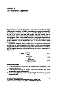
FIG. 1. Reconstruction of parameter a of logistic map: confidence intervals of reconstruction as a function of w 共the horizontal line is for the “correct” value of a兲. The time series with the noise level of 0.4 is used for reconstruction.

共i.e., as long as informativity of posterior distribution is increasing兲. Examples of the dependence of w on the enumerated factors will be given in Secs. III and IV. Note that the modified Bayesian approach is adapted to DS reconstruction at the cost of increased number of latent variables: they are 共T − w兲 ⬎ T / 2 in expression 共7兲. Thus, when performing reconstruction by sufficiently extended TS containing measurement noise one can encounter the problem of an extremely large number of arguments for posterior probability density p共u , ␮ 兩 x兲. Solution of this problem needs special investigation. In the two sections to follow we will demonstrate efficiency of the modified Bayesian approach on examples of solution of problems in which this difficulty does not arise.

III. RECONSTRUCTION OF PARAMETER VALUES OF A KNOWN DS BY NOISY TS

The example from Ref. 关2兴 given at the end of Sec. I clearly shows the inapplicability of the classical Bayesian approach, if initial conditions are not known precisely. We will show now that the modified approach allows estimation of parameter, even if there is no a priori information about the value of latent variable. We remind the reader that for solution of this problem Meyer and Christensen proposed a different modification of the Bayesian approach, namely, they suggested replacing the dynamic system by the stochas-

tic one. For comparison with results of reconstruction obtained by Meyer and Christensen we took as observational data time series generated by a logistic map with the value of parameter a the same as in Ref. 关6兴 共a = 1.85兲 and the initial condition x0 = 0.3. The time series is corrupted by white Gaussian noise with the ␴noise / ␴signal ratio different for each series ranging from 0 to 2. An ensemble of values of parameter a, by which a 95% confidence interval was calculated, was generated by the MCMC method for each time series in accord with the posterior distribution 共7兲 for different segment lengths w within the 1-to-7 interval. The confidence interval of parameter a reconstructed by TS with the noise level of 0.4 is shown in Fig. 1 for different segment lengths w = 1 , . . . , 7. Clearly, in accord with the qualitative considerations given in Sec. I, an increase in w results in a decrease of both systematic bias relative to the correct parameter value and the distribution width determining error. Consequently, for the segment length w = 2, the correct value of the parameter lies within the 95% confidence interval and at w = 7 the bounds of the confidence interval differ from the correct value by less than 1%. Variation of the confidence interval of parameter a with increasing noise level is shown in Fig. 2 for different segment lengths. Clearly, the use of the modified posterior probability density 共7兲 with w ⬎ 3 gives a better accuracy of reconstruction than the Meyer and Christensen approach 共cf. an analogous dependence of the size of confidence interval on noise level in Ref. 关8兴兲. Thus, the modification of the Bayesian approach proposed in this paper seems to be more efficient. To conclude this section we note that, for moderately noisy TS, it can be shown that the width ␴a of the distribution 共8兲 is related to the largest Lyapunov exponent ␭ and segment length w by

␴a ⬀ e−␭w .

共9兲

Figure 3 demonstrates that the theoretical dependence 共9兲 ␴a vs w 共the straight line in Fig. 3; the value of ␭ was calculated by the logistic map TS using the TISEAN software 关12兴兲 is in good agreement with results of reconstruction 共the dots in Fig. 3兲.

FIG. 2. Reconstruction of parameter a of logistic map: 95% confidence interval of parameter a as a function of noise level ␴noise / ␴signal for different segment lengths w 共the horizontal line is for the “correct” value of a兲.

036211-4

PHYSICAL REVIEW E 73, 036211 共2006兲

MODIFIED BAYESIAN APPROACH FOR THE¼

FIG. 3. Reconstruction of parameter a of logistic map: ␴a versus w: the dots show results of reconstruction 共␴noise / ␴signal = 0.2兲, and the line is the theoretical dependence 共9兲. IV. CLASSIFICATION OF TYPES OF BEHAVIOR OF KNOWN DS BY SHORT NOISY TS

The results obtained in the preceding section enable us to formulate the problem of classification of types of DS behavior that is important from the practical viewpoint. Consider by way of example very short 共T = 20兲 TS generated by a more complex DS, namely, Henon map. Evolution operator of this DS is a second-order sequence function un+1 = vn , vn+1 = 1 − av2n − bun .

共10兲

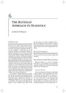
System 共10兲 may demonstrate diverse regular and chaotic modes of behavior, depending on values of parameters a and b. Regions of parameters corresponding to different modes of behavior are shown by graded gray colors in the bifurcation diagram 共Fig. 4兲.

FIG. 4. Bifurcation diagram of Henon map. The graded gray colors show modes corresponding 共from bottom to top兲 to stable equilibrium state, to two-period, four-period, and chaotic modes, and to the region of global instability of the model. The gray dots mark values of parameters at which the TS were generated. The ellipses are the boundaries of confidence intervals with 95% probability of parameter reconstruction for different w; ␴␰ = 0.06.

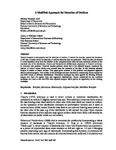
We took x as a “measurable” quantity, that is latent variable u with additive noise: xn = un + ␰n. Measurement noise ␰ was ␦-correlated and had Gaussian distribution with dispersion ␴␰2. We analyzed the TS generated for different values of parameters a and b. In the absence of noise, the TS corresponding to different periodic and chaotic modes are readily distinguishable. By way of example we present in Figs. 5共a兲 and 5共b兲 the TS generated by the map 共10兲 which correspond to two-period 共a = 1.05, b = −0.1兲 and chaotic 共a = 1.3, b = −0.2兲 modes. Addition of even relatively small noise 关see Figs. 5共c兲 and 5共d兲, ␴␰ = 0.3兴 makes the dynamic modes indistinguishable. We will demonstrate how this problem may be solved by means of the modified Bayesian approach. The problem of classification of the mode of behavior of the DS generating the initial noisy TS is based on investigation of a statistical ensemble of noiseless TS corresponding to a statistical ensemble of parameters distributed according to the posterior probability density 共8兲 关the ensemble is formed by means of the MCMC algorithm applied to the posterior distribution 共7兲兴. First, the number of elements of the ensemble of noiseless TS corresponding to one or another dynamic regime is counted, and then probability of each recorded mode is calculated. Probability of the “correct” mode of behavior as a function of noise level is plotted in Fig. 6 for the chaotic and one of periodic noisy TS generated by the map 共10兲. Note that closeness to unity of the probability of the most probable type of behavior is a convenient quantitative characteristic of the quality of classification. Let us now consider dependence of this characteristic on segment length w. From the above mentioned it is clear that, in the case of the chaotic behavior, this probability will generally approach unity with increasing w. Probabilities of erroneous types will decrease almost always due to decreasing width of posterior parameter distribution density with increasing w. Let us now try to understand whether this conclusion is true for the w dependence of the probability of “correct” regular mode. As was mentioned in Sec. II, factorization of the probability density 共5兲 implying a decrease in information coupling between the TS counts with increasing time interval between them becomes incorrect for the system functioning in a regular 共nonchaotic兲 mode. As a consequence of this incorrectness the dependence of parameter distribution width on w is somewhat different compared with the case of the chaotic mode. Namely, for regular regimes this dependence does not decay exponentially as in the case of chaotic mode 关see 共9兲兴. This is explained by the fact that there is no exponentially fast spreading of initially close phase trajectories on the attractor corresponding to a regular mode of a dynamic system; hence, there is no exponential growth of sensitivity of the current state of the system to initial conditions with increasing observation time. Nevertheless, reduction of the width of p共␮ 兩 x兲 with increasing w ensures an increase of the probability of correct mode with increasing segment length for regular modes of behavior too. The above mentioned is confirmed by results of reconstruction of system 共10兲 presented in Figs. 4 and 6. Figure 4 shows confidence regions of system parameters reconstruction by the corresponding noisy TS. One can see that for w ⬍ 4 the quality of classification improves with increasing

036211-5

PHYSICAL REVIEW E 73, 036211 共2006兲

MUKHIN et al.

FIG. 5. 共a兲 and 共b兲 Chaotic and periodic TS corresponding to the values of parameters marked by dots in Fig. 2; 共c兲 and 共d兲 the same TS but with noise ␴␰ = 0.3.

segment length for both chaotic and regular modes of behavior. The dependence, decaying exponentially with increasing w, of the value of the confidence region of the chaotic regime on segment length is plotted in Fig. 7 together with the same but nonmonotonic dependence for the regular, two-period regime. V. CONCLUSION

We considered the statistical Bayesian approach to reconstruction of dynamic systems by time series generated by these very systems. We believe that this is the most adequate approach to reconstruction of “real” dynamic systems which, first, are subject to irregular external forcing in the course of signal generation and, second, the signal itself is randomly perturbed during propagation and recording. The statistical approach aims not only at reconstructing DS evolution operator but also at constructing probability density of parameters of this operator that are regarded to be random quantities. One of the main difficulties in realizing this approach arises during reconstruction by chaotic time series. The exponentially fast diverging of phase trajectories on a chaotic attractor results in an increase of irregularity of probability density of parameters as the duration of the TS grows. Hence, it is impossible to construct parameter probability density even for relatively short TS. We proposed a modification of the classical Bayesian approach that makes it pos-

sible to overcome this difficulty. The efficiency of the modified approach was demonstrated on an example of seeking unknown values of parameters of a known DS and classification of DS modes of behavior, both regular and chaotic, by short noisy TS. The significant “technical” limitation for applying the modified approach is the absence of a “fast” algorithm of constructing an arbitrary distribution function 共probability density兲 that depends on a very large number of arguments. For noisy TS, this number depends, primarily, on the TS length 共the number of latent variables兲. In Sec. II we showed that, within the framework of the modified Bayesian approach, information about dynamic features of the system can be retained to a considerable extent by using almost maximum possible number of latent variables for the considered TS. Thus, the proposed solution to the first problem makes development of an effective algorithm for calculation of multidimensional distribution functions still more essential. We hope to complete this task in the near future. To conclude we would like to emphasize universality of the proposed approach to reconstruction of DS. It may be used for any problems of information retrieval from TS generated by dynamic systems. A challenging problem of this kind is prognosis of qualitative behavior of unknown DS by chaotic TS. General formulation of this problem 共“prognosis of bifurcations”兲 was given in Ref. 关5兴 where this problem was solved successfully by means of “transforming” the dynamic system to a formally stochastic one: the defect of the

FIG. 6. Probability of recognition of “correct” dynamic mode as a function of noise level for different w: 共a兲 chaotic TS; 共b兲 periodic TS.

036211-6

PHYSICAL REVIEW E 73, 036211 共2006兲

MODIFIED BAYESIAN APPROACH FOR THE¼

proposed modified Bayesian approach corresponding to the maximum short segment w = 1. The results discussed in Secs. III and IV give us grounds to believe that the quality of bifurcation prognosis may be improved by increasing w up to a maximum possible value. Note that the example of constructing bifurcation prognosis given in Ref. 关5兴, similarly to all the other examples available in the literature 关13–16兴, refers to the case of “ideal,” free of measurement noise TS generated by a low-dimensional DS. No advance has been made in this problem so far because of the absence of effective algorithm for constructing multidimensional probability density arbitrarily depending on its arguments. FIG. 7. Area of 95% confidence interval versus segment length for chaotic 共the line with dots兲 and periodic 共the line with crosses兲 TS.

ACKNOWLEDGMENTS

model, inevitable by virtue of unknown DS, was described in Ref. 关5兴 as additive dynamic “noise.” The algorithm of bifurcation prognosis used in Ref. 关5兴 is a particular case of the

The work was done under support of the Russian Foundation for Basic Research 共Contract No. 02-02-17080兲 and the Complex Program of Research “Fundamental Problems of Nonlinear Dynamics” under the umbrella of the Presidium of the Russian Academy of Sciences 共project 3.3兲.

关1兴 V. S. Anishchenko and A. N. Pavlov, Phys. Rev. E 57, 2455 共1998兲. 关2兴 K. Judd, Phys. Rev. E 67, 026212 共2003兲. 关3兴 H. D. I. Abarbanel, Analysis of Observed Chaotic Data 共Springer-Verlag, New York, 1997兲. 关4兴 H. Kantz and T. Schreiber, Nonlinear Time Series Analysis 共Cambridge University Press, Cambridge, 1997兲. 关5兴 Y. I. Molkov and A. M. Feigin, Nonlinear Waves’2002 共Institute of Applied Physics, Nizhny Novgorod, 2002兲, pp. 34–52 共in Russian兲. 关6兴 B. P. Carlin and T. A. Louis, Bayes and Emperical Bayes Methods for Data Analysis 共Chapman and Hall, London, 1996兲. 关7兴 W. Gilks, S. Richardson, and D. Spiegelhalter, Markov Chain Monte Carlo in Practice 共Chapman and Hall, London, 1996兲. 关8兴 R. Meyer and N. Christensen, Phys. Rev. E 62, 3535 共2000兲. 关9兴 P. E. McSharry and L. A. Smith, Phys. Rev. Lett. 83, 4285 共1999兲. 关10兴 H. Bock, Recent Advances in Parameter Identification Techniques for O.D.E., Numerical Treatment of Inverse Problems

in Differential and Integral Equations 共Birkhauser, Basel, 1983兲. V. F. Pisarenko and D. Sornette, Phys. Rev. E 69, 036122 共2004兲. R. Hegger, H. Kantz, and T. Schreiber, Chaos 9, 413 共1999兲. A. M. Feigin, Y. I. Molkov, D. N. Mukhin, and E. M. Loskutov, Report No. 508, Institute of Applied Physics, 1999 共in Russian兲. A. M. Feigin, Y. I. Molkov, D. N. Mukhin, and E. M. Loskutov, Radiophys. Quantum Electron. 44, 348 共2001兲. A. M. Feigin, Y. I. Molkov, D. N. Mukhin, and E. M. Loskutov, Faraday Discuss. 120, 105 共2002兲. A. M. Feigin, Proceedings of the International Symposium “Topical Problems of Nonlinear Wave Physics” 共Nizhny Novgorod, Russia, 2003兲. For the TS considered in Ref. 关2兴 关the TS generated by system 共4兲 at a = 1.85; u0 = 0.3兴, ␴␰ = 0.1 corresponds approximately to the 6:1 signal-to-noise ratio. Note that, formally, for w = T expression 共5兲 transforms to the “classical” expression 共3兲.

关11兴 关12兴 关13兴

关14兴 关15兴 关16兴

关17兴

关18兴

036211-7