Krist V. Gernaey, Jakob K. Huusom and Rafiqul Gani (Eds.), 12th International Symposium on Process Systems Engineering and 25th European Symposium on Computer Aided Process Engineering. c 2015 Elsevier B.V. All rights reserved. 31 May - 4 June 2015, Copenhagen, Denmark.
Modified Minimum Variance Approach for State and Unknown Input Estimation Yukteshwar Baranwal, Pushkar Ballal and Mani Bhushan∗ Department of Chemical Engineering, Indian Institute of Technology Bombay, India-400076 *
[email protected]
Abstract For several systems of interest, inputs to the system may be unknown. Thus, one may be interested in estimating the unknown inputs alongwith the states. In this work, we modify the approach proposed by Madapusi and Bernstein (2007) for estimating the states and the unknown inputs. The approach, applicable to systems with feedthrough, obtains a minimum variance unbiased estimate of the states. The inputs are estimated after the filtered states are obtained and do not require any restrictive assumptions about the dynamic variation of the inputs. Compared to Madapusi and Bernstein (2007), our approach differs in the prediction step. In particular, we use the estimated input in the prediction step while it has not been considered in the work of Madapusi and Bernstein (2007). Our proposed modification reduces the number of constraints that need to be satisfied by the filter gain thereby increasing the applicability of the approach. The efficacy of the approach is demonstrated by applying it to estimate unknown inputs and states in a self powered neutron detector, that is widely used in nuclear reactors to monitor the neutron flux. Keywords: State estimation, unknown input estimation, minimum variance estimation, self powered neutron detector.
1. Introduction The problem of state estimation is to estimate the states of the system using an uncertain process model and noisy measurements. Most of the state estimation approaches available in literature assume that the inputs to the process are exactly known. However, in several systems of interest the inputs are not directly measured and hence their exact values are unknown. Relatively less attention has been given to problem of state estimation under this scenario. One approach for addressing such problems would be to consider the unknown input to be an unknown parameter and assume a dynamic model (typically random walk) for its variation. The problem is then to estimate the augmented states with parameter as an additional state. However, arbitrary assumptions about the dynamic variation of the unknown input may be poorly justified specially for inputs varying over a wide range in a deterministic manner. There are relatively fewer approaches that don’t assume any model for the variation of the unknown input. In particular, Kitanidis (1987) developed an unbiased minimum variance estimator for the states in the presence of unknown inputs. Their approach requires the filter gain to satisfy a constraint that ensures that the effect of the unknown input is not felt on the estimated state. However, the focus of their work is on state estimation only and they did not discuss estimation of the unknown inputs. Sanyal and Shen (1974) have considered the problem of state and input estimation but assume the input to be a series of impulses of unknown magnitudes occurring after significant time lapses. Glover (1969) consider mainly estimation of unknown inputs and not the
2
Baranwal et al.
states themselves. But they assume the initial state to be zero. Madapusi and Bernstein (2007) have presented observability conditions for estimating both states and unknown inputs. They also extend the work of Kitanidis (1987) to deal with feedthrough systems. In both the approaches of Kitanidis (1987) and Madapusi and Bernstein (2007), the prediction step in the filter implicitly assumes the unknown input to be zero. In this work, we focus on the problem of simultaneous state and unmeasured input estimation. Our work is applicable to linear systems with feedthrough, namely where the unmeasured inputs directly affect the measurements. In particular, we modify the approach of Madapusi and Bernstein (2007) in that we use the estimated value of the unmeasured input in the state prediction step at the next time instant. We show that this modification enables application of the approach to a larger class of systems by reducing the constraints to be satisfied by filter gain to ensure unbiased state estimates. It also results in better (lower variance) state estimates. The approach is thus a modification of traditional Kalman filter and ensures unbiased, minimum variance state estimates while using the estimated values of unmeasured inputs in the state prediction step. The utility of the approach is demonstrated by applying it to the problem of estimating neutron flux in a nuclear reactor. The rest of the paper is structured as follows: in section 2 we present the problem statement and summarize the existing relevant work. The proposed extension is presented in section 3. The approach is applied to a neutron flux estimation problem in section 4. The paper is concluded in section 5.
2. Problem Statement and Existing Approaches Consider a discrete-time linear system with a linear measurement function, xk+1 = Ak xk + Hk ek + wk
(1)
yk = Ck xk + Gk ek + vk
(2)
where, xk ∈ Rn , yk ∈ Rm , ek ∈ R p , wk ∈ Rn , vk ∈ Rm are respectively the states, measurements, unknown inputs, process noise and measurement noise, respectively. wk and vk are usually considered to be white, Gaussian discrete time stochastic processes with mean 0 and covariances Qk and Rk respectively. The subscript k for the various quantities indicates the time instant tk . The problem in joint state and unknown input estimation is to obtain the best estimates of xk and ek given the measurements upto time tk . Note that while writing the measurement equation above, we have assumed direct feedthrough namely that the unmeasured inputs ek directly affect the measurements yk . Further, for simplicity of notation we have not considered known inputs in either the state evolution or measurement equation. Incase some known inputs are present, the proposed methodology can easily be modified to accommodate them. We now summarize the existing relevant technique (Madapusi and Bernstein, 2007) for simultaneous state and unknown input estimation. 2.1. Simultaneous State and Input Estimation We assume the conditional state density at time tk to be Gaussian with mean xˆk|k and covariance Pk|k . In the approach proposed by Kitanidis (1987) and Madapusi and Bernstein (2007), the filter takes the following form: xˆk+1|k = Ak xˆk|k xˆk+1|k+1 = xˆk+1|k + Lk+1 (yk+1 −Ck+1 xˆk+1|k )
(3) (4)
where xˆk+1|k+1 is the required filtered (estimated or updated) state while Lk+1 is the filter gain and xˆk+1|k is the model predicted state based on measurements till time instant k − 1. An important thing to note in the prediction equation (Eq. 3) is that the effect of the unknown input has been ignored while predicting the state.
Modified Minimum Variance Approach for State and Unknown Input Estimation
3
Define the state estimation error as: εk+1|k+1 , xk+1 − xˆk+1|k+1 . Requiring the state estimation error to be 0 mean, leads to the following constraints on the filter gain (Madapusi and Bernstein, 2007): (I − Lk+1Ck+1 )Hk = 0
(5)
Lk+1 Gk+1 = 0
(6)
The updated error covariance matrix Pk+1|k+1 is given by, T T T T Pk+1|k+1 , E[εk+1|k+1 εk+1|k+1 ] = Lk+1 R˜ k+1 Lk+1 − Fk+1 Lk+1 − Lk+1 Fk+1 + Pk+1|k
(7)
where, T T Pk+1|k = Ak Pk|k ATk + Qk , R˜ k+1 = Ck+1 Pk+1|kCk+1 + Rk+1 , Fk+1 = Pk+1|kCk+1
(8)
The unbiased minimum-variance gain Lk+1 is calculated by minimizing the trace of the error covariance matrix Pk+1|k+1 subject to the constraints in Eq. 5 and 6 and is given by, −1 T ˜ −1 Lk+1 = (Fk+1 + Ωk+1 (ΦTk+1 R˜ −1 k+1 ΦK+1 ) ΦK+1 )Rk+1
(9)
where, Φk+1 = [−Gk+1
Vk+1 ], Vk+1 = Ck+1 Hk , Ωk+1 = [0n×p
Hk ] − Fk+1 R˜ −1 k+1 Φk+1
(10)
This completes the state estimation step. The estimate eˆk of the unknown input is subsequently obtained as (Madapusi and Bernstein, 2007), eˆk+1|k+1 = G†k+1 (yk+1 −Ck+1 xˆk+1|k+1 )
(11)
where, G† is Moore-Penrose generalized inverse, given G† = (GT G)−1 GT . Note that the presence of the unknown input e(k) in the measurement equation (Eq. 2) enables its estimation using the above expression. Further, it can be shown (Madapusi and Bernstein, 2007) that Eq. 11 provides an unbiased estimate of the unknown input i.e. E[e¯k+1|k+1 ] = 0 where e¯k+1|k+1 , ek+1 − eˆk+1|k+1 is the error in estimating the unknown input.
3. Proposed Approach In this work, we propose the following filter form, xˆk+1|k = Ak xˆk|k + Hk eˆk|k xˆk+1|k+1 = xˆk+1|k + Lk+1 (yk+1 −Ck+1 xˆk+1|k )
(12) (13)
Comparing with Eqs. 3 and 4, it can be seen that our approach does not ignore the unknown input while predicting the states. Instead, we use the estimated value of the unknown input eˆk|k in the prediction equation. The expected value of the state estimation error εk+1|k+1 then can be derived to be, E[εk+1|k+1 ] = E[(I − Lk+1Ck+1 )Ak εk|k + (I − Lk+1Ck+1 )Hk (ek − eˆk|k ) + (I − Lk+1Ck+1 )wk − Lk+1 Gk+1 ek+1 − Lk+1 vk+1 ]
(14)
Now the filter gain can be derived using a similar procedure as in Kitanidis (1987); Madapusi and Bernstein (2007). If the estimated inputs and the estimated states at previous time step are
4
Baranwal et al.
unbiased, we have E[ek − eˆk|k ] = 0 and E[εk|k ] = 0. Further, since the unknown input ek is arbitrary, the following condition needs to hold for obtaining unbiased state estimates at time tk+1 : Lk+1 Gk+1 = 0
(15)
Comparing this condition to Eqs. 5 and 6, it can be seen that the proposed approach results in less restrictive conditions on the filter gain. Further, it can be noted that for the filter gain to exist, the matrix Gk+1 should have a non-empty left null space i.e. the number of measurements should be more than the number of unknown inputs. Using constraint 15, the state estimation error is, εk+1|k+1 = (I − Lk+1Ck+1 )(Ak εk + Hk e¯k|k + wk ) − Lk+1 vk+1 Thus, the covariance matrix Pk+1|k+1 of state estimation errors can be derived to be, i h T T T T = Pk+1|k − Lk+1 Fk+1 − Fk+1 Lk+1 + Lk+1 R˜ k+1 Lk+1 Pk+1|k+1 = E εk+1|k+1 εk+1|k+1
(16)
where, T Pk+1|k = Ak Pk|k ATk + Hk ξk+1 HkT + Ak σk+1 HkT + Hk σk+1 ATk + Qk
ξk+1 = E[e¯k|k e¯Tk|k ] = G†k (Ck Pk|kCkT
+ Rk −Ck Lk Rk − Rk LkT CkT )(G†k )T
(−Pk|kCkT + Lk Rk )(G†k )T T T R˜ k+1 = Ck+1 Pk+1|kCk+1 + Rk+1 , Fk+1 = Pk+1|kCk+1 σk+1 = E[εk|k e¯Tk ] =
(17) (18) (19) (20)
As in the previous section, the optimal filter gain is now computed by minimizing the trace of the estimation error covariance matrix, i.e. trace(Pk+1|k+1 ), subject to constraint in Eq. 15 and is given by, T −1 T ˜ −1 ˜ −1 Lk+1 = Fk+1 (I − R˜ −1 k+1 Gk+1 (Gk+1 Rk+1 Gk+1 ) Gk+1 )Rk+1
(21)
Once the state is estimated, the estimate of the unknown input can be computed as, eˆk+1|k+1 = G†k+1 (yk+1 −Ck+1 xˆk+1|k+1 )
(22)
It can be shown that this is an unbiased estimate of the unknown input. We label our approach as modified input reconstruction (MInpR) approach to distinguish it from the input reconstruction approach presented in the last section.
4. Case Study We now implement the proposed approach on a self powered neutron detector (SPND) which is a sensor widely used in nuclear reactors for incore neutron flux estimation. An SPND operates on the principle of activation by neutron interaction, namely that it generates current upon absorption of neutrons. A dynamic model of Vanadium SPND is (Srinivasarengan et al., 2012): d N52 (t) = −λ52 N52 (t) + σ51 N51 φ (t) dt I(t) = k pv σ51 N51 (t)φ (t) + kgv λ52 N52 (t)
(23) (24)
where state N52 denotes the concentration (atoms.cm−3 ) of the isotope 52V , while φ denotes the neutron flux (neutrons.cm−2 .sec−1 ) which is the unknown input of interest. The measurement I(t) is of the current generated by the SPND. Note that while writing this model, the concentration N51 of the stable isotope 51V has been assumed to be a constant. The various parameters occurring in the above equations are listed in Table 1. The constants kgv , k pv reported in this Table have
Modified Minimum Variance Approach for State and Unknown Input Estimation
5
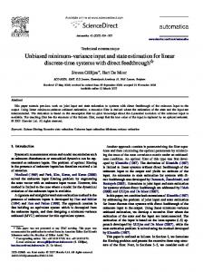
been multiplied by a factor of 1 × 10⁹ to scale the measurement. The sampling interval for the measurements is 1 second. It can be seen that the above is a direct feedthrough linear state space model since the input φ (t) directly appears in the measurement equation as well. However, the size of the G matrix (Eq. 2) is 1 × 1. From Eq. 15, this directly leads to filter gain being zero and the proposed approach (Sec. 3) or the existing approach in literature (Sec. 2) cannot be applied. We thus consider two Vanadium SPNDs with the same, but unknown input. In a nuclear reactor, such a scenario is possible since a typical nuclear reactor has several SPNDs some of which are highly correlated (Razak et al., 2014). The parameters of both the SPNDs are assumed to be the same as given in Table 1. While the proposed modified input reconstruction approach can be applied to estimate states and the unknown input, an analysis of Eqs. 5 and 6 reveals that these constraints cannot be simultaneously satisfied and hence the existing input reconstruction approach cannot be applied. We thus apply the proposed MInpR approach and compare its results with a covariancereset approach presented in Srinivasarengan et al. (2012). The latter assumes a random walk model for the unknown flux and applies a traditional Kalman filter to the augmented system. However to track sudden changes in the flux, it heuristically resets the variance of the estimated flux to a large value when the mean of norm of the innovations in a moving window exceeds a predefined threshold. Thus, tuning parameters related to the length of the window, the threshold and the value to which the variance is reset, need to be suitably chosen for the approach to work properly. Three types of input (flux) profiles are generated. The corresponding inputs estimated by the covariance-reset approach and the proposed MInpR approach are shown in Fig. 1 alongwith the true input profiles. The mean squared errors (MSE) corresponding to the estimated fluxes and the estimated states are reported in Table 2. From this table it can be seen the state estimation accuracy is higher (i.e. MSE is lower) with the proposed approach for all the three flux profiles. The accuracy of estimated flux profiles is higher for the covariance-reset approach for first two flux profiles while it is higher for the proposed approach for the third flux profile. Table 1: Model Parameters Parameter N51 σ51 λ52 kgv k pv
Values 6.86 × 10²² 4.9 × 10⁻²⁴ 3.6 × 10⁻³ 3.846 × 10⁻²⁰ 3.487 × 10⁻¹²
Unit cm−3 cm2 sec−1 Amperes.sec Amperes.sec
Table 2: MSE for Estimated States and Inputs Flux Profile Flux 1
Flux 2
Flux 3
Variable State: sensor 1 State: sensor 2 Flux State: sensor 1 State: sensor 2 Flux State: sensor 1 State: sensor 2 Flux
KF (Cov Reset) 1.1068 × 10¹⁴ 1.1822 × 10¹⁴ 5.4099 × 10¹² 0.7972 × 10¹⁴ 0.7997 × 10¹⁴ 6.2910 × 10¹² 0.9375 × 10¹⁴ 1.0180 × 10¹⁴ 8.6614 × 10¹²
MInpR 1.0590 × 10¹⁴ 1.1284 × 10¹⁴ 6.7876 × 10¹² 0.7204 × 10¹⁴ 0.7298 × 10¹⁴ 6.5288 × 10¹² 0.8040 × 10¹⁴ 0.8890 × 10¹⁴ 7.1141 × 10¹²
5. Conclusions In this work, we present a technique for estimating states and unknown inputs for linear systems with feedthrough. The technique, labeled modified input reconstruction approach, modifies an existing (Madapusi and Bernstein, 2007) technique from literature. The modification is in the prediction step and reduces the number of constraints to be satisfied by the filter gain while obtaining
6
Baranwal et al.
x 10
13
KF(Cov Reset) flux1 (neutron/cm2/sec)
flux1 (neutron/cm2/sec)
13
12
True Flux Estimated Flux
10 8 6 4 2 0
10 20 time (min)
30
12
flux2 (neutron/cm2/sec)
flux2 (neutron/cm2/sec)
True Flux Estimated Flux
8 6 4 2 0
8 6 4 2 0
10 20 time (min)
30
12
flux3 (neutron/cm2/sec)
flux3 (neutron/cm2/sec)
True Flux Estimated Flux
8 6 4 2 0
30
x 10
True Flux Estimated Flux
8 6 4 2 0
10 20 time (min)
30
13
x 10
10
10 20 time (min)
10
13
12
True Flux Estimated Flux
13
x 10
10
MInpR
10
13
12
x 10
10 20 time (min)
30
12
x 10
True Flux Estimated Flux
10 8 6 4 2 0
10 20 time (min)
30
Figure 1: Flux Estimation for Vanadium SPND unbiased, minimum variance estimates of the states. The approach is applied to estimate states and the unknown input for a self powered neutron detector, which are widely used in nuclear reactors. The results demonstrate superior quality of state estimation when compared to traditional estimation approach that assumes a dynamic model for the variation of the unknown input, while the quality of estimated inputs is comparable. However, unlike the traditional approach, the proposed approach does not involve any tuning parameters.
References Glover, J. D., 1969. The linear estimation of completely uknown signals. IEEE Transactions on Automatic Control 14, 766–767. Kitanidis, P. K., 1987. Unbiased minimum-variance linear state estimation. Automatica 23 (6), 775 – 778. Madapusi, H., Bernstein, D., 2007. Unbiased minimum-variance filtering for input reconstruction. In: Proceedings of the American Control Conference, ACC ’07. pp. 5712–5717. Razak, R. A., Bhushan, M., Belur, M. N., Tiwari, A. P., Kelkar, M. G., Pramanik, M., 2014. Clustering of self powered neutron detectors: Combining prompt and slow dynamics. IEEE Transactions on Nuclear Science, accepted for publication. Sanyal, P., Shen, C. N., 1974. Bayes’ decision rule for rapid detection and adaptive estimation scheme with space applications. IEEE Transactions on Automatic Control AC-19, 228–231. Srinivasarengan, K., Mutyam, L., Belur, M., Bhushan, M., Tiwari, A., Kelkar, M., Pramanik, M., 2012. Flux estimation from vanadium and cobalt self powered neutron detectors (spnds): Nonlinear exact inversion and kalman filter approaches. In: Proceedings of American Control Conference, ACC ’12. pp. 318–323.