Apr 4, 1999 - In the early 1970s, single-unit recordings from. Manuscript received .... The PFC has been demonstrated to have a modular or. Table 1.
IEICE TRANS. FUNDAMENTALS, VOL.E82–A, NO.4 APRIL 1999
688
PAPER
Modular Circuitry and Network Dynamics for the Formation of Visuospatial Working Memory in the Primate Prefrontal Cortex Shoji TANAKA† , Member and Shuhei OKADA† , Nonmember
SUMMARY A model of the prefrontal cortical circuit has been constructed to investigate the dynamics for working memory processing. The model circuit is multi-layered and consists of a number of circuit modules or columns, each of which has local, excitatory and inhibitory connections as well as feedback connections. The columns interact with each other via the longrange horizontal connections. Besides these intrinsic connections, the pyramidal and spiny cells in the superficial layers receive the specific cue-related input and all the cortical neurons receive a hypothetical bias input. The model cortical circuit amplifies the response to the transient, cue-related input. The dynamics of the circuit evolves autonomously after the termination of the input. As a result, the circuit reaches in several hundred milliseconds an equilibrium state, in which the neurons exhibit graded-level, sustained activity. The sustained activity varies gradually with the cue direction, thus forming memory fields. In the formation of the memory fields, the feedback connections, the horizontal connections, and the bias input all play important roles. Varying the level of the bias input dramatically changes the dynamics of the model cortical neurons. The computer simulations show that there is an optimum level of the input for the formation of well-defined memory fields during the delay period. key words: working memory, memory field, prefrontal cortex, column, closed-loop, neural circuit
1.
Introduction
The research of higher brain functions such as thought processes attracts not only psychologists and neuroscientists but researchers in engineering. In the last decade, working memory has been studied progressively and is now being under intensive investigation. Working memory is considered as a basic function of thought processes [1]–[3]. Many researchers have used so far various kinds of working memory tasks, such as visual, visuospatial, auditory, and verbal working memory tasks, in behavioral, neurophysiological, and functional mapping studies. These mapping experiments demonstrated that, for most of the tasks tested, the prefrontal cortex (PFC) in primates, including human, were commonly activated while performing those tasks. It is considered now that working memory processes arecentrally executed by the PFC [2]–[4]. In the early 1970s, single-unit recordings from Manuscript received December 24, 1997. Manuscript revised October 21, 1998. † The authors are with the Department of Electrical and Electronics Engineering, Sophia University, Tokyo, 102– 8554 Japan.
the monkey PFC during delayed-response performance showed sustained activity during the delay period for the first time [5], [6]. Since then, the relevance of the delay-period activity of PFC neurons to short-term or working memory has been argued [2], [7]. Later, deeper insights into the delay-period activity has been gained by neurophysiological studies employing oculomotor paradigms [8], [9]. For oculomotor delayedresponse tasks, Goldman-Rakic and coworkers observed from the monkey PFC that the delay-period activity has directional characteristics; that is, the firing frequency of the delay-period activity of a neuron reaches a maximum when the direction at which saccade to occur coincides with the preferred (or best) direction of the neuron and decreases in other directions [8], [9]. They termed this activity of the PFC neurons ‘memory fields’ and considered that the memory fields are neuronal substrate of the visuospatial working memory [8]. Their results strengthened the evidence that the PFC (especially the area within and surrounding the principal sulcus) is the principal area to form and maintain a visuospatial working memory. However, how the prefrontal cortex performs such mnemonic processes is not clear. The processes could be synergetic phenomena, which emerge from the dynamics of a circuit rather than from the action of a single neuron. Then the mechanisms would be attributable to the dynamical aspects of the circuit. To investigate this issue, computer simulations of the dynamics of the prefrontal cortical circuit can be useful and may compensate for the inaccessibility of experimental approaches by filling the gap between electrophysiological data and dynamics of the circuit. Zipser and coworkers demonstrated that a learning-based recurrent network model has gained gating properties and attractors by which the experimentally observed sustained activity in the inferotemporal cortex can be explained [10], [11]. However, the network they have developed cannot maintain the precise graded levels of activity indefinitely but eventually relaxes to one of the attractors. Therefore, their model is not suited to account for the formation of the memory fields in the PFC. We are interested in constructing a biologically plausible model of the PFC circuit for oculomotor visuospatial working memory processing [12]. With this
TANAKA and OKADA: MODULAR CIRCUITRY AND NETWORK DYNAMICS
689
model, we investigate here the processes for the formation of memory fields that have been observed in experiments. Because the lifetimes of the working memory processes are usually of the order of seconds, synaptic modification would not be expected to occur while performing a single working memory task. Instead, a change would occur in the signal flow in the circuit underlying a working memory process. This would then cause dynamic and synergetic modification of neuronal activity. This paper will address this issue that is supposed to be an essential aspect of the working memory process. 2.
Table 1 Connectivity of the model circuit. The symbol ‘F’ in the table indicates intrinsic, forward or horizontal connections from a neuron in a famiry (either PS, B, or PD) in the first line to a neuron in a family in the left column, ‘Rb’ denotes the intrinsic, feedback connections, ‘Rs’ indicates the self-feedback connections, and ‘A’ indicates the afferent inputs which are either specific cue-related (Cue) or bias (Bias). The numbers in the table indicate the numbers of the synapses (in total, the model circuit contains 22,568 synapses).
Model Circuit
2.1 Cortical Neurons and Connections The PFC contains, as the other neocortical areas, pyramidal and spiny nonpyramidal cells, which are excitatory, and various types of smooth cells, which are inhibitory [13]. Our model of the prefrontal cortical circuit classifies these cells into three families, namely PS cells, B cells, and PD cells. PS cells denote pyramidal (and spiny nonpyramidal) cells in the superficial layers, B cells denote inhibitory nonpyramidal neurons, and PD cells denote pyramidal cells in the deep layers. As in other cortical areas, inhibitory interneurons in the PFC include basket cells, double bouquet cells, chandelier cells, etc. [13]. However, our model does not distinguish further the types of these cells. In this paper, the intrinsic connections as well as the extrinsic inputs are modeled in the following way: (a) PS cells make forward and horizontal connections with B and PD cells, (b) B cells inhibit PD cells by local connections, (c) collaterals of PD cells send feedback projections to PS cells, (d) all the cortical neurons make self-feedback connections, (e) a specific cue-related signal is input to PS cells, and (f) all the cortical neurons receive a bias input. These connections are summarized in Table 1. The circuit diagram of a small part of the model circuit is shown in Fig. 1. The symbols in the figure are simplified to avoid unnecessary complexity in the diagram. The pyramidal cells are symbolized in the figure by triangular cell bodies and long upright dendrites. The B cells are symbolized by circular cell bodies with short dendrites. The rather thin lines denote the axons and the arrow heads denote the synapses. The intrinsic circuits are drawn with the lines having rounded corners. Horizontal fibers run horizontally in the superficial layers of the cortex in the figure. The diagram does not specify exact locations of the synapses on the dendrites. 2.2 Circuit Modules or Columns The PFC has been demonstrated to have a modular or
Fig. 1 Circuit diagram of a small part of the model. The figure shows two identical circuit modules, each of which corresponds to a column. PS: pyramidal (and spiny nonpyramidal) cells in the superficial layers (excitatory), B: smooth neurons (inhibitory), PD: pyramidal cells in the deep layers (excitatory).
columnar organization, as the other sensory and motor areas of the cortex [14], [15]. Figure 1 shows two of the columns or the circuit modules. Our model PFC is composed of 104 columns. Each column contains three neurons, belonging to different families (PS, B, and PD). Thus the model cortex contains 312 neurons in all. Because every column contains no more than a single neuron for each family, it does not take into account the intracolumnar connections between the same cell families. An arrangement of these columns constitutes the whole model cortical circuit. Since the columns have various directional preferences (or preferred directions), they may function as ‘directional columns’ in the mnemonic processing, like the orientation column in the visual cortex. A schematic diagram of the directional columns and the excitatory connections between
IEICE TRANS. FUNDAMENTALS, VOL.E82–A, NO.4 APRIL 1999
690
puter Simulations, a PD cell has the same preferred direction with that of the PS cell in the same column, while the B cell in the same column has the preferred direction opposite to that of the PS cell.) Once the preferred directions of the PS cells are assigned, they can label the columns in which the PS cells reside. In the following, therefore, we use the preferred directions of the PS cells to specify the column, such that the column of the PS cell with the preferred directions θi is specified by the column of the preferred direction of θi or simply the column i. 2.3 Horizontal Connections
Fig. 2 Directional columns (circles) and the strength of the excitatory intercolumnar connections. The arrows in the circles denote the characteristic directions of the columns. The size of the squares denote the relative strengths of the excitatory intercolumnar connections.
these columns are shown in Fig. 2. The connectivity profile will be given in Sect. 2.3. The ensemble of the columns with various preferred directions underlies the population coding of the memorized target direction. Experiments by Goldman-Rakic and coworkers showed that the preferred directions of the PFC cells during both the cue period and the delay period were widely distributed [8], [9], [16]. They also showed that the distribution of the preferred directions of the cortical cells in one hemisphere tended to be weighted so that more neurons have preferred directions toward the contralateral visual field and fewer neurons have preferred directions toward the ipsilateral visual field or along the vertical meridian [8], [9], [16]. The distribution of the preferred directions of the neurons in the other hemisphere is weighted in the opposite direction. It is then reasonable to postulate that the neurons in both the hemispheres constitute a whole population, connected with each other via interhemispheric as well as intrahemispheric fibers. In the whole population, therefore, the preferred directions would be distributed almost uniformly in the whole directional space. This would be necessary in order to code direction evenly without any bias to a certain direction. It is consistent with the population coding theory of direction, which requires uniformly distributed preferred directions [17]. In our model, the preferred directions of the PS cells are generated from uniformly distributed pseudorandom numbers from 0◦ to 360◦ because only the neurons of this family receive the cue-related signal (see below). The preferred directions of neurons in the other families need not be assigned; instead, they are determined dynamically by the circuit. (As will be shown in 4. Com-
The horizontal extension of the connections in the PFC has been investigated experimentally [18], [19]. The experimental results show that the horizontal connections are strongest in layers II and III, though some were observed to be in the deep layers. Besides the direct pyramidal to pyramidal connections (termed here the PP connections), electron microscopic studies clarified the pyramidal to smooth connections (termed here the PB connections) and the smooth to pyramidal connections (termed here the BP connections) as well [3]. In our model, therefore, the PS cells are assumed to make horizontal connections to both the B cells and the PD cells. Horizontal projections from the PD cells are, on the contrary, neglected. This differentiation in the connectivity of the PS and PD cells is just simplification of the model. As a result of this, the PD cells do not have axonal collaterals that extend horizontally; instead, all of the PD cells are assumed to have collaterals making intracolumnar feedback connections with PS cells (see Local Connections). Experiments demonstrated that each hemisphere has a population of PFC neurons exhibiting delay-period activity [8], [9] and that the same regions in both the hemispheres are interconnected [20]. Then the horizontal (PB and PP) connections in our model include not only intrahemispheric connections but interhemispheric ones. In the visual cortex, many experiments have confirmed that the connections between neurons with similar preferred orientations are stronger than the others [21]–[25]. Moreover, Katz and coworkers observed (i) that the largest-amplitude excitatory and inhibitory responses were evoked in single neurons when stimulation and recording electrode were located in orientation columns sharing the same angle preference and (ii) that both excitatory and inhibitory responses gradually decreased in amplitude when the difference between the preferred orientations of the stimulation and the recording columns gradually increased until they were orthogonal [25]. In the motor cortex, Georgopoulos and coworkers observed that the strongest excitatory connections were between the neurons with similar directional preferences, the negatively strongest connections were between those whose preferred directions
TANAKA and OKADA: MODULAR CIRCUITRY AND NETWORK DYNAMICS
691
were anti-parallel with each other, and the weakest or no connections were between those with the preferred directions perpendicular to each other [26]. No such data has been obtained from the PFC as far as the author knows. However, it has been suggested that neurons with similar response preferences in the PFC are interconnected [3], [18], [27]. Our model, therefore, assumes the above rule of connectivity. To argue the connectivity profile quantitatively, let us introduce the preferred direction space extending over 360◦. In this space, we can define a connectivity function, which specifies the strength of the connections from one neuron to another. In general, the connectivity function can have any waveform, having any higher harmonic modes as well as the fundamental mode in the Fourier series. However, the information on the higher harmonic modes is limited at present. Therefore, we will discuss only the fundamental mode as well as the zeroth mode or the constant value of the connectivity function. The connectivity function having only these modes is able to describe the iso-directions connectivity profile (i.e., the strongest excitatory connections between the columns with closest preferred directions). For the excitatory connection from PS cell k to PD cell i, the connectivity is weakest for the connections between the columns with anti-parallel preferred directions. The weakest connectivity is practically regarded to be zero in our model. Therefore, the connectivity profile for the PP connections is given by PP = wP P [1 + cos(θk − θi )] wki
(1)
rapidly decay to zero with the increasing differences between the preferred directions of the column in which the B cell resides and that in which the target cell resides. Consequently, our model neglects the intercolumnar projections. Besides these, polysynaptic intracolumnar connections could exist. However, they are modeled here only implicitly (see below). We thus describe the profile of the local inhibitory connectivity as BP = wBP δli wli
(3)
where δli is the Kronecker delta (δli = 1 for l = i; δli = 0 for l �= i) and wBP is a constant. 2.4.2
Intrinsic Feedback Connections
Tracing techniques have revealed that collaterals of the pyramidal cells in the deep layers of the PFC go upward and have synaptic terminals in the superficial layers [18], [19]. The techniques have also revealed downward interlaminar connections from the superficial to the deep layers. Therefore, the cortical circuit contains reciprocal connections between the superficial and the deep layers. The downward projections have already been modeled (i.e., the projections from PS cells to PD cells). Then we here model the upward projections by assuming that the collaterals of PD cells project to the PS cells in the same columns. 2.4.3
Self-Feedback Connections
PP
where w is a constant. On the contrary, the PB connection from a PS cell to a B cell should be strongest between the columns whose preferred directions are antiparallel. That is because the PD cells that receive the strongest inhibitory influences from the B cells in the same columns should have their preferred directions opposite to those of the PS cells having the strongest excitatory influences on the B cells. Therefore, the connection from PS cell k to B cell i is given by PB wki
=w
PB
[1 − cos(θk − θi )]
(2)
2.4 Local Connections 2.4.1
Local Inhibitory Connections
Inhibitory neurons in the cortex make local connections with pyramidal cells and other nonpyramidal cells. Because the precise circuitry is not known yet, we simply assume that B cells send outputs to PD cells in the same column as well asto themselves (the self-feedback connections). There may also be a local projection from a B cell to PD cells. The intracolumnar projection from a B cell to the PD cell would be stronger than anyother intercolumnar projections. However, the effective strength of the intercolumnar projections would
Like the canonical microcircuit model of the visual cortex proposed by Douglas and Martin [28], all the cortical neurons in our model have the collaterals synapting upon themselves (i.e., the self-feedback connections). 2.5 Cue-Related Input At the beginning of an oculomotor delayed-response task, the subject is required to fixate the central spot. A visual cue is displayed in oculomotor delayedresponse tasks, indicating the target position to which the eyes move after the delay period. The cue is turned off immediately (usually several hundred milliseconds after the onset), beginning the delay period. Disappearance of the fixation spot at the end of the delay period instructs the subject to saccade to the target position displayed before the delay period. The cue signal would be processed first in the visual system of the brain, and the cue-related signal generated is ultimately input to a population of neurons in the PFC via specific afferent fibers. The responses of the neurons to the cue-related signal are transient (the firing rate increases rapidly and then decreases rapidly) and their duration is shorter than the cue period (usually around 100 ms) [9]. The directional selectivity of the responses
IEICE TRANS. FUNDAMENTALS, VOL.E82–A, NO.4 APRIL 1999
692
have been observed to be broad [9]. Then, considering that the cue-related signal is also tuned broadly in the directional space, we describe the cue-related input signal as (4) Ik (θ, t) = [I0 + I1 cos(θ − θk )]u(t) 0, t < 0 or t > τ 2t τ , 0≤t< (5) u(t) = τ 2 − 2(t − τ ) , τ ≤ t ≤ τ τ 2 where θ is the target direction, τ is the duration of the input to the PFC (τ = 100 ms in our model), and I0 , I1 , and θk are constants. The input is set to begin at t = 0 ms. The time course of the cue-related afferent signal is depicted in Fig. 3. Because our model assumes that PS cells receive the cue-related inputs, the PS cells would have directional selectivity in the response. The response would be maximum when θ = θk ; therefore, θk (k = 1, 2, . . .) is the preferred direction of the PS cell in the column k. 2.6 Bias Input To sustain the activity of the cortical neurons during the delay period, a certain mechanism should exist to amplify or boost the activity of the neurons. As a model of the mechanism, we assume a bias input that has the following characteristics: (i) The input is given equally to all the cortical neurons and (ii) the strength or action of the input is independent of both the stimulus target direction and the direction of the intended eye movement. At the end of the delay period, the level of this input should be lowered because the sustained activity is turned off at the time. Experiments have shown that this activity is seen occurring in a synchronized manner in many neurons [8], [9]. The time course of the input is, therefore, given by � t < td ∆I0 , ∆I = ∆I1 + (∆I0 − ∆I1 )e−(t−td )/τd , t ≥ td (6)
Fig. 3 Temporal profile of the cue-related input signal (i.e., u(t) of Eq. (5)). Our model assumes that PS cells receive this input.
where ∆I0 , ∆I1 , and τd are constants and td is the time at which the strength of the bias input is changed. In the following, our computer simulations will show that the formation, maintenance, and erasing of memory fields are controlled by this input. 3.
Model Neurons
We employ a single compartment model to describe the dynamics of the firing rate of cortical neurons [29]. The firing events are not described explicitly, since we are interested in the dynamics whose time scale is much longer than that of the active potential. Instead, our model assumes that the excitatory and inhibitory synaptic inputs are proportional to the firing rates of the presynaptic neurons. The equations thus obtained describe the dynamics of the firing rates of the model neurons (see below). The model neurons have a threshold for firing and nonlinearity in the input-output relationship including saturation at high input levels, which is described by an activation function (see below). The model neurons have no adaptation mechanisms. Notations used in our model are listed in Table 2. 3.1 PS Cells According to the connectivity modeled in the last section, the dynamics of the internal state variable of the PS cell k, VkP S (t), is described by the differential equation: CP S
d PS D Rb V (t) = Ik + Rb aP k (t − ∆t ) dt k S Rs PS + RsP S aP k (t − ∆t ) + ∆I PS − gleak [VkP S (t) − Eleak ] (7)
The internal state variable above the firing threshold is converted to the firing rate by S PS aP k (t) = f [Vk (t) − Vth ]
Table 2
Symbols used in this article.
(8)
TANAKA and OKADA: MODULAR CIRCUITRY AND NETWORK DYNAMICS
693
where f (•) is the activation function, which is defined by � amax tanh(x/h), x > 0 (9) f (x) = 0, x≤0
The transmission and synaptic delays for the PP, PB, and BP connections (∆tP P , ∆tP B and ∆tBP , respectively), for the self-feedback connection (∆tRs ), and for the feedback connection from a PD to a PS cell (∆tRb ) are all taken to be 2 ms.
Here amax is the maximum firing frequency and h is the slope of the activation function, denoting the efficiency of the input for firing (the smaller, the more efficient).
4.
3.2 B Cells The dynamics of the internal state variable of the B cell is similarly described by the differential equation: CB
� d B PB PS Vl (t) = wkl ak (t − ∆tP B ) dt k
Rs B + RsB aB l (t − ∆t ) + ∆I B − gleak [VlB (t) − Eleak ]
(10)
And the firing rate of the B cell is given by B aB l (t) = f [Vl (t) − Vth ]
(11)
3.3 PD Cells The differential equation for the internal state variable and the equation for the firing rate of the PD cell are: CP D
� d PD PP PS Vi (t) = wki ak (t − ∆tP P ) dt k � BP B − wli al (t − ∆tBP ) l D (t − ∆tRs ) + ∆I P D + RsP D aP i PD − gleak [ViP D (t) − Eleak ] (12)
and D aP (t) = f [ViP D (t) − Vth ] i
(13)
The time constants of change in the internal state variables are, from Table 3, τ = C/gleak = 20 ms for the PS and PD cell families and τ = C/gleak = 10 ms for the B cell family. Table 3 Values of the parameters used in the computer simulation.
Computer Simulations
4.1 Phasic Response To investigate the roles of the intracolumnar feedback connections (i.e., the collaterals of the PD cells projecting to the PS cells in the same columns) on the response to the cue-related input, we first simulate the responses of the model cortical neurons to the cuerelated input when the circuit has no such feedback connections. The neurons have self-feedback connections, whose strengths are given by −0.025 for the PS and PD cells and −0.01 for the B cells. The strength of the input, which has been modeled by Eq. (4), is specified by (I0 , I1 ) = (0.5, 0.25). All the cortical neurons receive the bias input: (∆I P S , ∆I B , ∆I P D ) = (0.330, 0.132, 0.330). The results depicted in Fig. 4 show that all the responses of the PS, B, and PD cells are phasic. The durations of the firing are not longer than that of the input (100 ms). The PS cell started to fire first because it receives the input first; the other two neurons delayed the start of firing by about 15 to 20 ms. However, the slower start of these cells is considered to be due not to the transmission and synaptic delay (which is 2 ms) but to synergetic phenomena of the circuit, because the delay is much longer than 2 ms. Actually, the transmission and synaptic delay is much shorter than the time constant of the internal state variables, which are 20 ms for the PS and PD cells and 10 ms for the B cells. Then the simulation results change only slightly when the synaptic delay is neglected. The B cell started to fire last, and the firing frequency increased and decreased faster than the other neurons, so that the duration of the firing of the B cell is shorter than for the other neurons. This is a direct result of the simulation; no assumption was made on this. The activity patterns shown in the figure are those when the target direction coincides with the preferred directions of the sample neurons. For target directions that do not coincide with the preferred direction of the PS and PD cells or the direction opposite to the preferred direction of the B cell, the responses of the neurons are weaker than those shown in the figure depending on the difference between the two directions. 4.2 Memory Fields Next, we will see the responses of the cortical neurons to the same cue-related input when the circuit has intracolumnar feedback connections, whose strength is given by 0.04. Figure 5 shows the responses of three PD
IEICE TRANS. FUNDAMENTALS, VOL.E82–A, NO.4 APRIL 1999
694
Fig. 4 The responses of PS, B, and PD cells of the circuit without the feedback connections to the cue-related input. The activity patterns shown in the figure are those when the target direction coincides with the preferred directions of the sample neurons. A: PS cell, B: B cell, C: PD cell.
Fig. 5 Tonic responses of three PD cells of the circuit with the feedback connections to the cue-related input. The preferred directions of these neurons are A: 0◦ , B: 90◦ , and C: 180◦ , respectively, while the cue-related signal represents the target direction of 0◦ .
cells, whose preferred directions are 0◦ , 90◦ , and 180◦ , respectively, while the cue-related signal represents the target direction of 0◦ . The activity is sustained when the preferred direction is not far away from the target direction. The activity patterns of the other cell families are not shown because they are similar to those of the PD cell. The circuit dynamics determine the activity pattern of the cortical neurons. The maximum firing rate of the tonic activity occurs when the preferred direction of the neuron coincides with the target direction (Fig. 5A), and this activity is much greater than that without the feedback connections. This activity shows an initial rapid increase of the firing rate followed by a gradual increase (from t ≈ 100 ms to t ≈ 500 ms). This slow change of the activity is also seen for the 90◦ cell (Fig. 5B), though the amount of the change is small. In the cell with the preferred direction of 180◦ (Fig. 5C), it emerges as a gradual decrease of the firing rate, showing a short-lived response to the input. Even in this case,
the response is not the same as the response without the feedback connections. With the feedback connections, the activity continues for about 270 ms after the end of the input, while, without the feedback connections, it never lasts well after that. These three cells belong to the same population of the model PFC, so that the data are obtained by a single run of the computer simulation. During the course of the operation of the circuit, the strength of the bias input changed from (∆I P S , ∆I B , ∆I P D ) = (0.330, 0.132, 0.330) for t ≤ 1800 ms to (∆I P S , ∆I B , ∆I P D ) = (0, 0, 0) with the time constant of 30 ms (τd = 30 ms, and td = 1800 ms in Eq. (6)). The time course of the input to the PD cells is shown in Fig. 6. The termination of the bias input turns off the tonic activity. When the strength of the bias input suddenly decreases to a certain level above zero, the decay of the firing rate becomes slower, though these results are not shown here. The tonic activity observed here indicates the for-
TANAKA and OKADA: MODULAR CIRCUITRY AND NETWORK DYNAMICS
695
Fig. 6 Time course of the strength of the bias input to the PD cells, which is given by Eq. (6). The values of the parameters are: ∆I0 , = 0.330, ∆I1 ,= 0, τd = 30 ms, and td = 1800 ms.
Fig. 7 Directional profiles of the memory fields of a set of PS, B, and PD cells in a single column (the thin solid curve: PS cell, the dashed curve: B cell, the thick solid curve: PD cell). The snapshot is taken at 1000 ms after onset of the cue-related input to the PFC circuit.
mation of memory fields. It is consistent with the experimental observations [8]. The directional profiles of the memory fields are shown in Fig. 7, in which the firing rates of the PS, B, and PD cells in the same column at t = 1, 000 ms are plotted for various target directions. Note that the PS and PD cells have a preferred direction of 0◦ , while the B cell has a preferred directions of 180◦ , opposite to those of the PS and PD cells in the same column. This is reasonable when one considers the inhibitory action of the B cell. This opposite polarization of the memory fields of a pair of pyramidal cells and an inhibitory cell has been observed experimentally [30]. The rapid increase of the firing frequency during the first 100 ms, shown in Fig. 5A, indicates that the process in this stage is a direct consequence of the cuerelated input. To see this initial process, we take several snapshots of the memory fields of the cortical neurons in this period of time. Figure 8 shows the memory fields of a set of PS, B, and PD cells in a single column at different times. The PS cell starts to fire first, then the PD cell starts to fire, as in the case without feedback connections (Fig. 4). In the very early stage of the response (Fig. 8A), therefore, the firing frequency of the PS cell is higher than that of the PD cell. In this stage, the B cell does not fire at all. The
Fig. 8 Directional profiles of the premature memory fields of a set of PS, B, and PD cells in a single column at different times (A: t = 40 ms, B: t = 55 ms, C: t = 100 ms).
B cell increases its firing rate rapidly after this stage. At t ≈ 55 ms (Fig. 8B), the activity levels of the three cells become comparable (the tuning curves of the PS and PD cells almost overlap). After t ≈ 55 ms, the PD cell increases its firing rate faster than the PS cell, and the B cell continues to increase its firing rate progressively (Fig. 8C). In this stage, however, the profiles of the memory fields of these neurons are still flatter than those at t = 1000 ms (Fig. 7), indicating that shaping is not completed. Shaping has progressed further at the late stage (t > 100 ms), in which the depth of directional tuning of the memory fields of these cells increases gradually. Shaping is completed at t ≈ 500 ms in our model. After that, the activity becomes invariant, thus forming the memory fields shown in Fig. 7.
IEICE TRANS. FUNDAMENTALS, VOL.E82–A, NO.4 APRIL 1999
696
Fig. 9 Time course of the activity of a PD cell for various strengths of the bias input. The strengths of the bias input are: from the lowest to the highest, 0.269 (lowest; the solid line), 0.330 (lower middle; the thick solid line), 0.500 (higher middle; the dashed line), and 1.000 (highest; the dashed line). Among these four cases, the appropriate formation of memory fields are shown only for the bias input, ∆I P D = 0.330.
Fig. 10 Tuning curves of the memory field of a PD cell for various bias input, which are: 0.269 (solid thin curve, lowest), 0.275 (solid thin curve, lowest but one), 0.330 (solid thick curve), 0.350 (dashed curve with lowest tails), 0.365 (dashed curve with lowest peak value), 0.500 (dashed curve, largest but one), and 1.000 (dashed curve, largest).
4.3 Changing the Strength of the Bias Input The last subsection has shown that the bias input plays a critically important role in sustaining the neuronal activity. In this subsection, we will see how the dynamics and the memory change when the strength of the bias input varies. Figure 9 shows the activity patterns of the PD cell for various strengths of the bias input when the target direction coincides with the preferred direction. The activity pattern depicted by the thick solid line for the bias input of 0.330 is the same as that shown in Fig. 4A. For an excessive level of the input (≥ 0.5), the increase of the firing rate at the initial stage of the activity is very sharp and high-frequency activity is maintained thereafter. The sustained firing rate is not very much higher than the normal one, but the directional selectivity of the activity during the delay period is quite different. In the high-input operation (for the bias input of above about 0.5), all the cortical neurons (PS, B, and PD) lose their directional selectivity as can be seen from the flat tuning curves in Fig. 10. However, the window of the level of the input for which memory fields with a considerable degree of directional selectivity are formed and stably maintained is not so narrow. With the set of parameter values for the present simulation, it is estimated to be 0.27 < ∆I P D < 0.35. Above the higher end of the window, the memory fields lose directional selectivity as mentioned above. Slightly below the lower end of the window, on the contrary, memory fields are not maintained during the full delay period. Similar results have been obtained for PS and B cells. This is interesting because experiments have shown that, in those cases, the subject generally makes an error [8]. To see the effects of the bias input on the memory field profiles, the tuning curves for the memory fields of a PD cell for the various strengths of the bias input are depicted in Fig. 10. When the bias input is in the lower range (∆I P D ≤ 0.33), increase of the bias input causes potentiation of the memory field. In the middle
rage (0.33 < ∆I P D < 0.5), additional increase of the bias input decreases the peak value of the memory field, while the background level is increased. This indicates a decreasing of the signal-to-noise ratio of the activity. An increase in the bias input beyond ∆I P D ≈ 0.5 results in complete loss of the directional selectivity of the memory field. A further increase in the bias input just shifts the tuning curve upward, indicating that the cortical neuron exhibits nonselective high-frequency firing. 5.
Network Dynamics
5.1 Formation of Memory Fields Our computer simulations have shown the formation processes of memory fields of the model PFC neurons. The cue-related input into the circuit causes the initial rapid increase of the activity, which is followed by a gradual increase lasting for about several hundred milliseconds. The circuit reaches an equilibrium state well after the end of the cue-related input. This suggests that the formation of memory fields is mainly due to autonomously evolving dynamics of the circuit triggered by the cue-related input. This dynamics is inherent to the network which is appropriately designed; no single neuron in this model does not have such dynamics. Moreover, Fig. 4A shows that the peak value of the firing rate of the PD cell without the feedback connections is about 13 sp/s, while the firing rate of the same cell reaches above 40 sp/s within the first 100 ms when the circuit has appropriate feedback connections (Fig. 5A). This indicates that amplification of the input signal occurs in the cortical circuit. The dynamics of the PFC circuit evolves further via the feedback connections and the horizontal connections. In the latter stage (100 ms < t < 500 ms), the interaction among the columns via the horizontal connections changes the ac-
TANAKA and OKADA: MODULAR CIRCUITRY AND NETWORK DYNAMICS
697
tivity gradually. After that, the dynamics of the circuit with adjusted values of the parameters for these connections and the bias input reach a stable equilibrium state, maintaining the graded levels of activity for the memory fields. The shape of the memory fields usually reflects the profile of the cue-related input signal, which has been formulated by using a cosine function in our model. Funahashi et al. [8] used Gaussian distribution functions to fit the data for the memory fields. The results were that the standard deviations were 26.8◦ ± 14.2◦ (SD) for neurons with significant excitatory delay-period activity and 48.2◦ ± 43.5◦ (SD) for neurons with only inhibitory delay-period activity. However, the data had only eight sampling points with an interval of 45◦ because the target was chosen from those eight points on the screen. The sampling theorem shows that, in those cases, higher harmonics whose wavelengths are shorter than 90◦ are filtered out [31]. Therefore, neither the actual shape nor the width of the memory fields can be completely extracted from their data. On the contrary, the cosine function is the fundamental mode of any waveform and has been widely used in fitting data from the motor cortical neurons [17],[32]–[34]. A numerical study has suggested that the fundamental mode dominates the performance of the directional coding by a population of neurons, while the higher harmonic modes are less important in the directional population coding than the fundamental mode [35]. Therefore, in this study, we have used a cosine function to describe the cue-related signal instead of using a Gaussian distribution function. Theoretical and numerical analyses of the tuning functions with various widths, shapes, and levels of non-signal component have been undertaken [35]–[37]. 5.2 Roles of the Bias Input These computer simulations have shown that an appropriately regulated bias input to the cortical neurons plays an essential role in the formation and maintenance of memory fields. Varying the level of the bias input changes the dynamics of the PFC circuits considerably. The formation, maintenance, and erasing of memory fields is important as well because working memory is transitory in nature and its formation and erasing should be controlled dynamically for successive operations. Our computer simulations have shown that the erasing of memory fields can also be controlled by changing (lowering) the strength of the bias input. Therefore, the whole process of the mnemonic activity can be controlled by appropriately regulating the bias input in our model. Note that the bias input itself does not form memory fields because it causes only subthreshold events when the network receives no input. Instead, it modulates (even dramatically changes) the circuit dynamics. Therefore, it works as a modula-
tor for the circuit dynamics. It is a single-neuron view that the bias input simply increases or decreases the firing rate of the recipient neuron. To understand the dynamics of a neuronal circuit in which many neurons are interacting synergetically with each other, a more elaborate view is required. The computer simulations (Figs. 9 and 10) have shown that, with either an excessive or an insufficient amount of bias input, a directionally selective memory field does not form, and that there is an optimum level of the input for the formation of well-defined memory fields during the delay period. Insufficient bias input decreases the amplitude of the memory fields and does not maintain them during the full delay period (Fig. 9). When the circuit receives excessive input, on the contrary, high-frequency signals circulate throughout the circuit via the local and horizontal connections, making the dynamics unstable, whereby all the neurons exhibit high-frequency discharge with no directional selectivity (Fig. 10). Only appropriate levels of the input makes the circuit reach graded-level, equilibrium states. But the range of the bias input level by which the memory fields are formed and stably maintained is not so narrow, as mentioned in 4. Computer Simulations. This indicates rather robust dynamics of the circuit in the normal operation regime. 5.3 Closed-Loop Circuitry Our model circuit has postulated the forward connections (i.e., direct projections from PS cells to PD cells and indirect projections via B cells) and the backward connections (i.e., the intracolumnar feedback projections from PD cells to PS cells), thus forming closedloop circuitry. This closed-loop circuitry is necessary to sustain the activity of the cortical cells; without it the response to a transient cue-related signal is phasic. Besides the forward and backward connections, all the model cortical neurons have the self-feedback connections. The gain of the self-feedback connections is negative in our model. Because the actual cortical circuitry is more complex than our model, the negative self-feedback connections do not necessarily mean that a collateral of the axons of a PD cell, for example, projects bisynaptically to itself via a B cell. The reality may be that there exist multiple excitatory and inhibitory connections that function collectively as a self-feedback connection. Therefore, the negative gain of the self-feedback connection would imply that the inhibitory influence surpasses the excitatory influence so that the combined connectivity is inhibitory in effect. Extrinsic closed-loop circuitry may also be possible in which the outputs are sent to a subcortical structure, such as the mediodorsal thalamic nucleus, and then reentered to the cortex. Although not confirmed, this has been suggested for many years [5], [38]. The reentrant circuitry requires a longer time for the
IEICE TRANS. FUNDAMENTALS, VOL.E82–A, NO.4 APRIL 1999
698
circulation of signals than in the intrinsic closed-loop circuitry. Regarding this issue, I did a preliminary computer simulation for the model circuit having extrinsic closed-loop circuits with delays of 8 to 12 ms (distributed) and adjusted gains instead of the intrinsic closed-loop circuits with a delay of 2 ms. The results, not shown here, were very similar to those for the intrinsic closed-loop architecture as far as the formation and maintenance of memory fields are concerned. Further investigation with more elaborate modeling requires experimental data on neuronal circuitry and the dynamical properties of neurons in the PFC and subcortical structures closely connected with the PFC. 6.
Conclusion
We have developed a biologically plausible model of the PFC circuit and have investigated working memory processes for oculomotor delayed-response performance by doing computer simulations of the model. After receiving a transient cue-related signal, the cortical cells in the circuit model are shown to form and maintain ‘memory fields’ during the delay period. The memory field has been suggested in experiments to be a neuronal substrate for the working memory [8]. The circuit can also turn off the delay-period activity by changing the level of the bias input. Therefore, the formation, maintenance, and elimination of memory fields are controlled unitarily by regulating the nonspecific afferent inputs. In the formation of the memory fields, the closed-loop circuits, the horizontal circuits, and the bias input are critically important. In particular, changing the level of the bias input dramatically alters the dynamics of the model cortical neurons, suggesting that there are the optimum level of the input for the formation of well-defined memory fields during the delay period. For an insufficient level of the action, memory fields are not maintained during the full delay period. For an excessive level of the action, on the contrary, the whole population of the PFC neurons tends to exhibit high-frequency activity. But the window of the level of the action for which memory fields are formed and stably maintained is not so narrow. Our simulation found interesting cases in which memory fields disappeared in the midst of the delay period. The experiments showed that, in those cases, the subject generally makes an error [8]. In conclusion, the present model circuit has the dynamics that simulates the synergetic activity of a population of the PFC neurons during oculomotor delayed-response performance. Acknowledgements The author acknowledges valuable discussions with Prof. P.S. Goldman-Rakic at Yale University and Dr. S. Funahashi at Kyoto University. The author also thanks Profs. R. Deiters and M. Tanaka at Sophia Uni-
versity for giving useful comments on the model and its computer simulations and for commenting on the manuscript of this paper. Correspondence should be addressed to Dr. Shoji Tanaka, Department of Electrical and Electronics Engineering, Sophia University, 7–1 Kioicho, Chiyoda-ku, Tokyo 102–8554, Japan. The e-mail address is: tanakas@hoffman.cc.sophia.ac.jp. References [1] A. Baddeley, “Working memory,” Oxford Univ. Press, 1986. [2] P.S. Goldman-Rakic, “Prefrontal cortical dysfunction in schizophrenia: The relevance of working memory,” in Psychopathology and the brain, eds. B.J. Carroll and J.E. Barrett, pp.1–23. Raven, 1991. [3] P.S. Goldman-Rakic, “Cellular basis of working memory,” Neuron, vol.14, pp.477–485, 1995. [4] P.S. Goldman-Rakic, “Architecture of the prefrontal cortex and the central executive,” in Structure and functions of the human prefrontal cortex, eds. J. Graftman, K.J. Holyoak and F. Boller, Ann. New York Acad. Sci., vol.769, pp.71– 83, New York Acad. Sci., 1995. [5] J.M. Fuster and G.E. Alexander, “Neuron activity related to short-term memory,” Science, vol.173, pp.652–654, 1971. [6] K. Kubota and H. Niki, “Prefrontal cortical unit activity and delayed alternation performance in monkeys,” J. Neurophysiol., vol.34, pp.337–347, 1971. [7] J.M. Fuster, “Memory in the cerebral cortex,” MIT Press, 1994. [8] S. Funahashi, C.J. Bruce, and P.S. Goldman-Rakic, “Mnemonic coding of visual space in the monkey’s dorsolateral prefrontal cortex,” J. Neurophysiol., vol.61, pp.331– 349, 1989. [9] S. Funahashi, C.J. Bruce, and P.S. Goldman-Rakic, “Visuospatial coding in primate prefrontal neurons revealed by oculomotor paradigms,” J. Neurophysiol., vol.63, pp.814– 831, 1990. [10] D. Zipser “Recurrent network of the neural mechanisms of short-term active memory,” Neural Comput., vol.3, pp.179– 193, 1991. [11] D. Zipser, B. Kehoe, G. Littlewort, and J. Fuster, “A spiking network model of short-term active memory,” J. Neurosci., vol.13, pp.3406–3420, 1993. [12] S. Tanaka, S. Okada, K. Yoshizawa, and M. Edahiro, “Modular circuitry and network dynamics for working memory processing in primates,” Proc. 1997 International Symposium on Nonlinear Theory and its Applications, NOLTA’97, pp.181–184, 1997. [13] J.S. Lund and D.A. Lewis, “Local circuit neurons of developing and mature macaque prefrontal cortex: Golgi and immunocytochemical characteristics,” J. Comp. Neurol., vol.328, pp.282–312, 1993. [14] P.S. Goldman and W.J.H. Nauta, “Columnar distribution of cortico-cortical fibers in the frontal association, limbic, and motor cortex of the developing rhesus monkey,” Brain Res., vol.122, pp.393–413, 1977. [15] P.S. Goldman, “Modular organization of prefrontal cortex,” Trend. Neurosci., vol.7, pp.419–424, 1984. [16] S. Funahashi, C.J. Bruce, and P.S. Goldman-Rakic, “Neuronal activity related to saccadic eye movements in the monkey’s dorsolateral prefrontal cortex,” J. Neurophsyiol., vol.65, pp.1464–1483, 1991. [17] A.P. Georgopoulos, R.E. Kettner, and A.B. Schwartz, “Primate motor cortex and free arm movements to visual tar-
TANAKA and OKADA: MODULAR CIRCUITRY AND NETWORK DYNAMICS
699
[18]
[19]
[20]
[21]
[22]
[23]
[24]
[25]
[26]
[27]
[28]
[29] [30]
[31] [32]
[33]
[34]
gets in three-dimensional space. II. Coding of the direction of movement by a neuronal population,” J. Neurosci., vol.8, pp.2928–2937, 1988. J.B. Levitt, D.A. Lewis, T. Yoshioka, and J.S. Lund, “Topography of pyramidal neurons intrinsic connections in macaque monkey prefrontal cortex (areas 9 and 46),” J. Comp. Neurol., vol.338, pp.360–376, 1993. M.F. Kritzer and P.S. Goldman-Rakic, “Intrinsic circuit organization of the major layers and sublayers of the dorsolateral prefrontal cortex in the rhesus monkey,” J. Comp. Neurol., vol.359, pp.131–143, 1995. P.K. McGuire, J.F. Bates, and P.S. Goldman-Rakic, “Interhemispheric integration: I. Symmetry and convergence of the corticocortical connections of the left and the right prinsipal sulcus (PS) and the left and the right supplementary motor area (SMA) in the rhesus monkey,” Cerebr. Cortex, vol.1, pp.390–407, 1991. D.Y. Ts’o, C.D. Gilbert, and T.N. Wiesel, “Relationships between horizontal interactions and functional architecture in cat striate cortex as revealed by cross-correlation analysis,” J. Neurosci., vol.6, pp.1160–1170, 1986. C.D. Gilbert and T.N. Wiesel, “Columnar specificity of intrinsic horizontal and corticocortical connections in cat visual cortex,” J. Neurosci., vol.9, pp.2432–2442, 1989. C. Schwarz and J. Bolz, “Functional specificity of a longrange horizontal connections in cat visual cortex: A crosscorrelation study,” J. Neurosci., vol.11, pp.2995–3007, 1991. Y. Hata, T. Tsumoto, H. Sato, K. Hagihara, and H. Tamura, “Development of local horizontal interactions in cat visual cortex studied by cross-correlation analysis,” J. Neurophysiol., vol.69, pp.40–56, 1993. M. Weliky, K. Kandler, D. Fitzpatrick, and L.C. Katz, “Patterns of excitation and inhibition evoked by horizontal connections in visual cortex share a common relationship to orientation columns,” Neuron, vol.15, pp.541–552, 1995. A.P. Georgopoulos, M. Taira, and A. Lukashin “Cognitive neurophysiology of the motor cortex,” Science, vol.260, pp.47–52, 1993. M.L. Pucak, J.B. Levitt, J.S. Lund, and D.A. Lewis, “Patterns of intrinsic and associational circuitry in monkey prefrontal cortex,” J. Comp. Neurol., vol.376, pp.614–630, 1996. R.J. Douglas and K.A.C. Martin, “A functional microcircuit for cat visual cortex,” J. Physiol., vol.440, pp.735–769, 1991. C. Koch and I. Segev, eds., “Methods in neuronal modeling,” MIT Press, 1989. F.A. Wilson, S.P. O’Scalaidhe, and P.S. GoldmanRakic, “Functional synergism between putative gammaaminobutyrate-containing neurons and pyramidal neurons,” Proc. Natl. Acad. Sci. USA, vol.91, pp.4009–4013, 1994. J.S. Lim and A.V. Oppenheim, eds., “Advanced topics in signal processing,” Prentice-Hall, 1988. R. Kettner, A.B. Schwartz, and A.P. Georgopoulos, “Primate motor cortex and free arm movements to visual targets in three-dimensional space. III. Positional gradients and population coding of movement direction from various movement origins,” J. Neurosci., vol.8, pp.2938–2947, 1988. A.B. Schwartz, R. Kettner, and A.P. Georgopoulos, “Primate motor cortex and free arm movements to visual targets in three-dimensional space. I. Relations between single cell discharge and direction of movement,” J. Neurosci., vol.8, pp.2913–2927, 1988. J.F. Kalaska, D.A.D. Cohen, M.L. Hyde, and M. Prud’Homme, “A comparison of movement direction-
[35]
[36]
[37]
[38]
related versus load direction-related activity in primate motor cortex, using a two-dimensional reaching task,” J. Neurosci., vol.9, pp.2080–2102, 1989. S. Tanaka, “Numerical study of coding of the movement direction by a population in the motor cortex,” Biol. Cybern., vol.71, pp.503–510, 1994. H.S. Seung and H. Sompolinsky, “Simple models for reading neuronal population codes,” Proc. Natl. Acad. Sci. USA, vol.90, pp.10749–10753, 1993. S. Tanaka and N. Nakayama, “Numerical simulation of neuronal population coding: Influences of noise and the tuning width on the coding error,” Biol. Cybern., vol.73, pp.447– 456, 1995. J.M. Fuster, “Firing changes in cells of the nucleus medialis dorsalis associated with delayed response behavior,” Brain Res., vol.61, pp.79–91, 1973.
Shoji Tanaka received B.E., M.E., and Ph.D. degrees from Nagoya University in 1980, 1982, and 1985, respectively. In 1985, he was a postdoctoral fellow at Japan Atomic Energy Research Institute, Tokai-mura, Japan. He joined the Department of Electrical and Electronics Engineering, Sophia University, Tokyo in 1986. He is currently an Associate Professor at the Department of Electrical and Electronics Engineering, Sophia University. During 1998–1999, he is a Visiting Scientist at Section of Neurobiology, Yale University School of Medicine, where he is doing collaborative research on working memory with Prof. Patricia S. Goldman-Rakic.
Shuhei Okada received B.E. from Sophia University, Tokyo, in 1998. He is a graduate student at the Program of Electrical and Electronics Engineering, Sophia University. He is currently studying computational neuroscience and neurosystems engineering.