Monotonicity and Convexity of Some Functions Associated with ...

Monotonicity and Convexity of Some Functions Associated with Denumerable Markov Chains and Their Applications to Queueing Systems Hai-Bo YU Academy of Mathematics and System Sciences Chinese Academy of Sciences, Beijing 100080, P. R. China E-mail: [email protected] Qi-Ming HE Department of Industrial Engineering, Dalhousie University Halifax, Nova Scotia, Canada B3J 2X4 E-mail: [email protected] Hanqin Zhang Academy of Mathematics and System Sciences Chinese Academy of Sciences, Beijing 100080, P. R. China E-mail: [email protected]

Abstract Motivated by various applications in queueing theory, this paper is devoted to the monotonicity and convexity of some functions associated with discrete-time or continuous-time denumerable Markov chains. For the discrete-time case, conditions for the monotonicity and convexity of the functions are obtained by using the properties of stochastic dominance and monotone matrix. For the continuous-time case, by using the uniformization technique, similar results are obtained. As an application, the results are applied to analyze the monotonicity and convexity of functions associated with the queue length of some queueing systems. Keywards: Markov chains, stochastic dominance, uniformization, queueing systems. AMS 2000 Subject Classification: Primary 60J27; 34E05 Brief Title: Convexity of Some Functions Associated with Markov Chains 1

1. Introduction In queueing analysis, the queue length of customers is an important performance measure. Quite often, we are interested in the information on the queue length as a function of time. For instance, we may like to know how the mean queue length changes as a function of time or, under what conditions, the mean queue length is a monotone, convex, or concave function of time. For many queueing models, the queue length process can be described by a Markov chain. Thus, the study of the queueing process for those queueing models is equivalent to the study of a Markov chain with a finite or countable (denumerable infinitely) state space, i.e., a denumerable Markov chain (see Kemeny, Snell, and Knapp [11]). The objective of this paper is to study the monotonicity, convexity, or concavity of some functions associated with denumerable Markov chains. There have been a large number of papers and some books in the literature dealing with the monotonicity of stochastic processes. For instance, Doorn [4] discussed the stochastic monotonicity of birth-and-death processes. Stoyan [21] studied the stochastic monotonicity of Markov processes with applications in queueing theory. By using some partial orderings defined on a set of matrices, HE [7] studied the monotonicity of the corresponding rate matrix R for the Markov chain of GI/M/1 type (see Neuts [16]). Lindvall [13] discussed the problem of the monotonicity and convexity of birth-and-death processes by using the coupling method. Shanthikumar and Yao [20] studied the strong stochastic convexity of parameterized random variables. In queueing theory, there have been a number of papers in the literature dealing with the monotonicity and convexity of the mean waiting time or the throughput of queueing systems. For example, Dyer [5] showed that the mean waiting time in the M/M/c queue is strictly decreasing and convex in c (the number of severs in the system). Weber [23] extended that result to the GI/G/c queue. Shanthikumar and Yao [19] showed that the throughput in the M/M/c/K queue is increasing and concave in arrival rate. Shanthikumar and Yao [20] established the strong stochastic convexity for the mean waiting time of the GI/G/1 queue. Wang [22] showed that the actual waiting time of the nth customer in the GI/G/1 queue is stochastically increasing and concave in n in the sense of the usual stochastically larger order. For many queueing systems, the queue length process can be characterized by a discrete-time or continuous-time denumerable Markov chain. For example, the queue length process in the M/M/c queue can be characterized by a birth-and-death process. 2

The queue length process in the M/G/1 or GI/M/c queue can be described by a Markov chain embedded at the departure epochs or at the arrival epochs (see Cohen [2] or Hsu [8]), respectively. Unlike the waiting time process, the study of the monotonicity and convexity of the queue length process is limited. Lindvall [13] showed the monotonicity and convexity of the mean queue length for the M/M/c queue under certain conditions. In this paper the monotonicity and convexity of some functions associated with Markov chains are investigated. Some general conditions for the monotonicity or convexity are found. Based on these results, conditions for some functions associated with the queue length of some queueing systems to be monotonic, convex, or concave in time are found. For convenience, the results of this paper are shown only for Markov chains with a countable state space, though all results hold for Markov chains with a finite state space. That explains why the word “denumerable” is used in the title of this paper. The rest of the paper is organized as follows. In Section 2 we provide the definitions of stochastic dominance and monotone matrix. Some general conditions for functions associated with Markov chains to be monotone, convex, or concave are given in Section 3. By using the uniformization technique (see Dijk [3], Gross and Miller [6] or Medhi [14]), the results are extended to the case of continuous-time Markov chains. In Section 4, the results obtained in Sections 3 are applied to a number of queueing systems such as the M/M/c, M/G/1, and GI/M/c queues. Conditions for some functions of the queue length to be monotone, convex, or concave are found. Some comments on future research are provided in Section 5. Throughout this the paper, we use Z+ to denote the set of nonnegative integers and R+ for the set of nonnegative real numbers. We use x(i) to denote the ith component of a vector x and ai,j to denote the (i, j)th entry of a matrix A. Let < x, y > denote the inner P product of two vectors x and y, i.e., < x, y >= ∞ i=0 x(i)y(i). The terms “increasing” and “decreasing” mean “non-decreasing” and “non-increasing”, respectively.

2. Stochastic Dominance and Monotone Matrix Let λ = (λ(0), λ(1), . . .) and µ = (µ(0), µ(1), . . .) be two probability distributions defined on Z+ , and P be a stochastic matrix. Definition 2.1 We say that λ dominates µ, denoted by λ ≥ d µ (or equivalently µ ≤d λ), if

k X i=0

λ(i) ≤

k X

µ(i), for all k ≥ 0.

i=0

3

(1)

Note that stochastic dominance of measures is similar to the stochastically larger order of probability distributions (see Ross [17], Shaked and Shanthikumar [18], or Stoyan [21]). An equivalent way to define λ ≥d µ is that < λ, f > ≥ (≤) < µ, f >

(2)

holds for all increasing (decreasing) function f (·) defined on Z + , where f (·) has a vector representation f = (f (0), f (1), · · · ). Definition 2.2 Let pi = (pi,0 , pi,1 , · · · ) denote the ith row of a stochastic matrix P , i ≥ 0. The matrix P is called monotone if p i ≤d pi+1 for i ≥ 0, or equivalently, for i ≥ 0, k X

pi,j ≥

j=0

k X

pi+1,j

for all k ≥ 0.

(3)

j=0

A monotone matrix has the following useful properties. Proposition 2.1 Assume that a stochastic matrix P = (p i,j )i,j≥0 is monotone, and λ and µ are two probability distributions defined on Z + . (i) If λ ≥d µ, then λP n ≥d µP n , for all n ≥ 0.

(4)

(ii) If λ ≥d µ, and function f (·) defined on Z+ is increasing (decreasing), then < λP n , f > ≥ (≤) < µP n , f >, for all n ≥ 0.

(5)

Proof. It is easy to see that, to prove (i), we only need to show λP ≥ d µP . If λ ≥d µ, let P P∞ P∞ P∞ P∞ 0 λ0 = λP and µ0 = µP . Then ∞ j=0 λ (j) = j=0 i=0 λ(i)pi,j = i=0 λ(i) j=0 pi,j = 1. P∞ 0 0 0 Similarly, we have j=0 µ (j) = 1. Thus, λ and µ are also probability distributions P defined on Z+ . Let ξi (k) = kj=0 pi,j . In view of the monotonicity of the matrix P , we know that ξi (k) is decreasing in i for all k ≥ 0. Hence, for k ≥ 0, k P

λ0 (j) =

j=0

≤

k P ∞ P

j=0 i=0 ∞ P

λ(i)pi,j =

µ(i)ξi (k) =

i=0

∞ P

λ(i)(

i=0 ∞ P

µ(i)(

i=0

k P

j=0 k P

pi,j ) =

pi,j ) =

j=0

∞ P

λ(i)ξi (k)

i=0 k P

µ0 (j).

j=0

Thus, λP ≥d µP . Part (ii) can be shown by part (i) and Eq.(2).

2

Remark 2.1 In definition 2.2, it is possible to define the monotonicity of P as p i ≥d pi+1 for i ≥ 0. Nonetheless, such a definition does not lead to results such as part (i) in 4

Proposition 2.1. In fact, if λ ≥d µ, then λP ≤d µP under the new definition. Thus, it is more difficult to compare {λP n , n ≥ 0} and {µP n , n ≥ 0}. Therefore, we shall not explore such monotonicity of P in this paper. Remark 2.2 Stochastic dominance and monotone matrix are related to Markov chain theory in the following manner. Suppose that the stochastic matrix P is monotone, then the discrete dominance theory (see Lindvall [13, p.134]) ensures the existence of Markov e = {Yen , n ≥ 0} governed by P such that, almost surely, chains Y = {Yn , n ≥ 0} and Y Yn ≥ Yen , for all n ≥ 0, e satisfy: λ ≥d µ. if the initial distributions λ of Y and µ of Y 3. Monotonicity and Convexity In this section, we investigate the monotonicity and convexity of some functions associated with Markov chains for both the discrete-time and continuous-time cases. Note that all Markov chains considered in Sections 3, 4 and 5 have a countable state space. In addition, we assume that Markov chains are irreducible and aperiodic in discrete-time case and are irreducible in continuous-time case. 3.1 The discrete-time Markov chain case Consider a discrete-time Markov chain Y = {Y n , n ≥ 0}. Let P = (pi,j ) be the transition probability matrix of Y. Let λ be the initial probability distribution of the Markov chain Y. Let E λ (·) be the expectation of Y when the initial distribution of Y is λ. Define hf (i) =

∞ X

pi,j [f (j) − f (i)], i ≥ 0,

(6)

j=0

for function f (·) defined on Z+ . Let hf = (hf (0), hf (1), · · · ). Then Eq.(6) can be rewritten as hTf = P f T − f T , where “T” denote the transpose of vector. It is readily seen that hf (i) is the mean-drift of the Markov chain Y with respect to function f (·) at the state i. Thus, we call hf the mean-drift function of Y with respect to f (·). For Markov chain Y with transition matrix P , it is well known that P {Y n = i} = (λP n )(i), i ≥ 0. Thus, we have Eλ [f (Yn )] =< λP n , f >. In this paper, we study the monotonicity and convexity of the function E λ [f (Yn )] for the Markov chain Y with an initial distribution λ. The objective is to find conditions under which the function Eλ [f (Yn )] is increasing, decreasing, convex, or concave in n. For continuous-time Markov 5

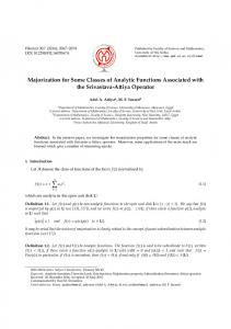
chain {X(t), t ≥ 0}, we want to find conditions under which the function E λ [f (X(t))] is increasing, decreasing, convex, or concave in t. The relationship between the functions Eλ [f (X(t))] and Eλ [f (Yn )] is given in Section 3.2. For example, consider an M/M/1 queue (see Section 4.1). The queue length process X = {X(t), t ≥ 0} is a birth-and-death process. The mean queue length E λ [X(t)] at time t is depicted in Figure 1 for different initial distribution λ. Figure 1 shows that the function Eλ [X(t)] can be monotone, convex, or concave if the initial distribution λ is chosen properly (Curves 1 and 2). Figure 1 also shows that, in general, the function Eλ [X(t)] may not be monotone, convex, nor concave (Curve 3). Thus, some conditions must be imposed on λ to ensure expected properties on E λ [X(t)]. In general, to ensure monotonicity, convexity, or concavity on the function E λ [f (Yn )], certain conditions must be imposed on the transition matrix P , the initial distribution λ, and the function f (·). The conditions considered in this paper are closely related to stochastic dominance of measures. Formally, we state the conditions as follows. Condition I :

P is monotone,

Condition II :

λP ≥d λ,

Condition II0 :

λ ≥d λP,

Condition III :

hf (i) defined in Eq. (6) is decreasing in i,

(7)

0

Condition III : hf (i) defined in Eq. (6) is increasing in i. The following theorem shows the monotonicity, convexity, and concavity of the function Eλ [f (Yn )] under the above conditions. The theorem also explains why the above conditions are utilized in this paper. Theorem 3.1 Consider an irreducible and aperiodic discrete-time Markov chain Y with transition matrix P . Let λ be the initial distribution of Y. Function f (·) is defined on Z+ . We assume that Eλ [f (Yn )] is finite for n ≥ 0. (i) If Conditions I and II in Eq.(7) hold and the function f (·) is increasing, then the function Eλ [f (Yn )] is increasing in n. If Conditions I and II in Eq.(7) hold and the function f (·) is decreasing, then the function E λ [f (Yn )] is decreasing in n. (ii) If Conditions I and II0 in Eq.(7) hold and the function f (·) is increasing, then the function Eλ [f (Yn )] is decreasing in n. If Conditions I and II 0 in Eq.(7) hold and the function f (·) is decreasing, then the function E λ [f (Yn )] is increasing in n. 6

(iii) If Conditions I, II and III in Eq.(7) hold, then the function E λ [f (Yn )] is concave in n. If Conditions I, II and III0 in Eq.(7) hold, then the function Eλ [f (Yn )] is convex in n. (iv) If Conditions I, II0 and III in Eq.(7) hold, then the function E λ [f (Yn )] is convex in n. If Conditions I, II0 and III0 in Eq.(7) hold, then the function Eλ [f (Yn )] is concave in n. Proof. We only give a proof to (iii). Others can be proved similarly. Since λ and P satisfy Condition I and Condition II in Eq.(7), by Proposition 2.1 we have λP n+1 ≥d λP n for all n ≥ 0. In view of the monotonicity of the mean-drift function h f , we obtain < λP n+1 , hf > ≤ < λP n , hf >. Hence, < λP n+2 , f > + < λP n , f > ≤ 2 < λP n+1 , f >, that is, Eλ [f (Yn )] is concave in n.

2

Remark 3.1 Assume that f (·) defined on Z + is increasing. f (·) satisfies Condition III in Eq.(7) if and only if the function ∆f is excessive (see C ¸ inlar [1, p.204]), where function ∆f is defined by ∆f (i + 1) = f (i + 1) − f (i), i ≥ 0. In general, it is not straightforward to check the conditions required in Theorem 3.1. Nonetheless, for some interesting special cases, these conditions can be checked (see Sections 4 and 5 for examples). We also point out that, in Theorem 3.1, the Markov chain Y does not have to be recurrent. Thus, in later sections, we do not require the Markov chains to be recurrent nor the queueing models to be stable, unless stated otherwise. Although the Markov chain Y in Theorem 3.1 is not required to be positive recurrent, some of the conditions in Eq.(7) have a close relationship with the positive recurrence of Y. For instance, if Y is positive recurrent, then Condition II implies λ ≤ d π, where π is the steady state distribution of Y. If the mean-drift function h f is negative and decreasing, then the Markov chain Y is positive recurrent by Foster’s criterion (see Cohen [2]). Such relationships are useful when we choose the initial distribution λ for our examples in Sections 4. 3.2 The continuous-time Markov chain case Based on the above results for discrete-time Markov chains, we can obtain similar results for continuous-time Markov chains by using the uniformization technique. Let X = {X(t), t ∈ R+ } be a homogeneous and continuous-time Markov chain. Let Q = (qi,j ) be the infinitesimal generator of X. Then Markov process X is said to be

7

uniformizable if sup(−qi,i ) < ∞. i≥0

If the Markov chain X is uniformizable, then for any ν ≥ sup (−qi,i ), we define i≥0

P =I+

1 Q, ν

(8)

where I is the identity matrix. Note that P defined by Eq.(8) is a stochastic matrix. We have (Medhi [14]): exp{Qt} = e

−νt

∞ X (νt)k k=0

k!

P k.

(9)

To study functions associated with X, we make use of a Markov chain with transition matrix P given in Eq.(8). We denote the Markov chain as Y. Assume that X and Y have the same initial distribution λ. Let g(λ, t) = Eλ [f (X(t)] =< λexp{Qt}, f >= e

−νt

∞ X (νt)k k=0

k!

< λP k , f > .

(10)

Suppose that the function g(λ, t) in Eq.(10) has derivative of order 2. Then by Eq.(8) and Eq.(9) we can establish the following relationships between X and Y: g(λ, t) = e−νt

∞ P

(νt)n n! Eλ [f (Yn )],

n=0 ∞ P

(νt) n n! [Eλ [f (Yn+1 )]

d dt g(λ, t)

=

νe−νt

d2 g(λ, t) dt2

=

n=0 ∞ P (νt)n 2 −νt ν e n! [Eλ [f (Yn+2 )] n=0

− Eλ [f (Yn )],

(11)

+ Eλ [f (Yn )] − 2Eλ [f (Yn+1 )]],

where Eλ [f (Yn )] is defined for the Markov chain Y. Eq.(11) indicates that, to study functions associated with X, it is sufficient to study functions associated with Y. More specifically, by Eq.(11), we know that the convexity of the function Eλ [f (Yn )] implies the convexity of the function E λ [f (X(t))]. Similarly, the monotonicity of the function E λ [f (Yn )] implies the monotonicity of the function Eλ [f (X(t))]. Counterparts of conditions in Eq.(7) are given as follows. Condition Icont :

I + Q/ν is monotone,

Condition IIcont :

λ(I + Q/ν) ≥d λ,

Condition II0cont : Condition IIIcont

λ ≥d λ(I + Q/ν), ∞ P : (Qf )(i) = qi,j f (j) is decreasing in i,

Condition III0cont : (Qf )(i) = 8

j=0 ∞ P j=0

qi,j f (j) is increasing in i.

(12)

We state the monotonicity, convexity, and concavity of the function E λ [f (X(t))] in the following theorem, it can be proved by combining Theorem 3.1 and Eq.(11), we omit its proof. Theorem 3.2 Consider a continuous-time Markov chain X with infinitesimal generator Q. Suppose that X is uniformizable, and let ν ≥ sup(−qi,i ). We assume that Markov i

chain Y with transition matrix P given by Eq.(8) is irreducible and aperiodic. Suppose that X and Y have the same initial distribution λ. We assume that E λ [f (X(t))] is finite for t ≥ 0. (i) If Conditions Icont and IIcont in Eq.(12) hold and if the function f (·) defined on Z + is increasing, then the function Eλ [f (X(t))] is increasing in t. If Conditions I cont and IIcont in Eq.(12) hold and if the function f (·) defined on Z + is decreasing, then the function Eλ [f (X(t))] is decreasing in t. (ii) If Conditions Icont and II0cont in Eq.(12) hold and if the function f (·) defined on Z + is increasing, then the function Eλ [f (X(t))] is decreasing in t. If Conditions I cont and II0cont in Eq.(12) hold and if the function f (·) defined on Z + is decreasing, then the function Eλ [f (X(t))] is increasing in t. (iii) If Conditions Icont , IIcont and IIIcont in Eq.(12) hold, then the function E λ [f (X(t))] is concave in t. If Conditions Icont , IIcont and III0cont in Eq.(12) hold, then the function Eλ [f (X(t))] is convex in t. (iv) If Conditions Icont , II0cont and IIIcont in Eq.(12) hold, then the function E λ [f (X(t))] is convex in t. If Conditions Icont , II0cont and III0cont in Eq.(12) hold, then the function Eλ [f (X(t))] is concave in t.

2

4. Applications to Queueing Systems In this section, we show how the monotonicity and convexity can help us gain insight into the queue length processes of a number of queueing systems. 4.1 The M/M/1 queue Consider an M/M/1 queue with an infinite number of waiting rooms, a first-in-first-served service discipline, arrival rate α, and service rate β (see Cohen [2]). We assume that α > 0 and β > 0. Let X(t) represent the number of customers in the system at time t. It is well

9

known that the queue length process X = {X(t), t ∈ R + } is a continuous-time Markov chain with an infinitesimal generator  −α α 0 0 0    β −(α + β) α 0 0   Q= 0 β −(α + β) α 0   0 β −(α + β) α  0  . . . .. .. .. .. .. . .

···



  ···    ··· .   ···   .. .

(13)

The Markov chain X with generator Q given by Eq.(13) is a special continuous-time Markov chain. The Markov chain X is irreducible and its discrete counterpart P defined by Eq.(8) is irreducible and aperiodic if α > 0 and β > 0. Let ν ≥ α + β and define ρ = α/β. Conditions in Eq.(12) can be simplified to Condition M/M/1(I) :

(α + β)/ν ≤ 1,

Condition M/M/1(II) :

λ(i + 1) ≤ ρλ(i), i ≥ 0,

0

Condition M/M/1(II ) :

λ(i + 1) ≥ ρλ(i), i ≥ 0,

Condition M/M/1(III) :

ρ∆f (i + 2) + ∆f (i) ≤ (1 + ρ)∆f (i + 1), i ≥ 0,

(14)

Condition M/M/1(III0 ) : ρ∆f (i + 2) + ∆f (i) ≥ (1 + ρ)∆f (i + 1), i ≥ 0. Note that for M/M/1(III) and M/M/1(III 0 ), we assume that ∆f (0) = 0, where ∆f is a function defined in Remark 3.1. To interpret the above conditions probabilistically, we use the following generalized likelihood ratio order defined for nonnegative measures. For two measures λ and µ, we say λ ≤lr µ if λ(i + 1)µ(i) ≤ λ(i)µ(i + 1) for i ≥ 0. For more about the likelihood ratio order for random variables see Shaked and Shanthikumar [18]. Let π ˆ = (1, ρ, ρ 2 , · · · ) and π ˆ −1 = (1, 1/ρ, 1/ρ2 , · · · ). If the queueing system is stable (i.e., ρ < 1), π ˆ can be normalized to a probability measure π = (1 − ρ, (1 − ρ)ρ, (1 − ρ)ρ 2 , · · · ), which is the steady state distribution of X. If ρ > 1, π ˆ −1 can be normalized to a probability measure π −1 = (ρ − 1)(1/ρ, 1/ρ2 , 1/ρ3 , · · · ). Proposition 4.1 Condition M/M/1(I) in Eq.(14) is satisfied for all ν ≥ α+β. Condition M/M/1(II) in Eq.(14) holds if and only if λ ≤ lr π ˆ . Condition M/M/1(II0 ) in Eq.(14) holds if and only if λ ≥lr π ˆ . Condition M/M/1(III) in Eq.(14) holds if and only if ∆ 2 f ≤lr π ˆ −1 , where function ∆2 f is defined by ∆2 f (i + 1) = ∆f (i + 1) − ∆f (i) for i ≥ 0. Condition M/M/1(III0 ) in Eq.(14) holds if and only if ∆2 f ≥lr π ˆ −1 . 10

Proof. It is clear that the first conclusion holds. The second and third conclusions hold by the definition of generalized likelihood ratio order defined above. The last two conclusions are true since, by Eq.(14), ρ∆ 2 f (i + 2) ≤ (≥)∆2 f (i + 1) for i ≥ 0.

2

Using Proposition 4.1, it is easy to check the conditions for the monotonicity and convexity of the function Eλ [f (X(t))]. For Condition M/M/1(II) or M/M/1(II 0 ) in Eq.(14), we consider the following initial distributions. ˆ 1 = (1, 0, 0, . . .), λ ˆ 2 = (0.3, 0.2, 0.1, 0.1, 0.1, 0.1, 0.1, 0, . . .), λ ˆ 3 = (0.1, 0.1, 0.1, 0.1, 0.1, 0.1, 0.1, 0.1, 0.1, 0.1, 0, . . .), λ 2 ˆ 4 = ( 1−ρ3 , (1−ρ)ρ , (1−ρ)ρ , 0, . . .), ρ < 1, λ 1−ρ 1−ρ3 1−ρ3 ˆ 5 = (1 − ρ, (1 − ρ)ρ, (1 − ρ)ρ2 , . . .), ρ < 1, λ ˆ 6 = (0, 0, 0, 1 − ρ, (1 − ρ)ρ, (1 − ρ)ρ2 , . . .), ρ < 1, λ

(15)

ˆ 7 = (0, 0, 0.01, 0.09, 0.19, 0.24, 0.47, 0, . . .), λ ˆ 8 = (0, 0, 0, 0, 0, 0.01, 0.09, 0.19, 0.24, 0.47, 0, . . .), λ ˆ 9 = (0, 0, 0, 0, 0, 0, 0, 0, 0.01, 0.09, 0.19, 0.24, 0.47, 0, . . .). λ ˆ 1 satisfies Condition M/M/1(II) in Eq.(14) By Proposition 4.1, it can be verified that λ ˆ 2 and λ ˆ 3 satisfy Condition M/M/1(II) if ρ ≥ 1; λ ˆ 4 and λ ˆ 5 satisfy Condition for all ρ ≥ 0; λ ˆ 5 and λ ˆ 6 satisfy Condition M/M/1(II0 ) in Eq.(14) if ρ < 1; λ ˆ7, λ ˆ8 M/M/1(II) if ρ < 1; λ ˆ 9 satisfy neither Condition M/M/1(II) nor Condition M/M/1(II 0 ). and λ For Condition M/M/1(III) in Eq.(14), we consider the function f (i) = i k , i ≥ 0, where k = 1, 2, · · · . By Proposition 4.1, if k = 1, Condition M/M/1(III) holds for all ρ > 0; if k = 2, Condition M/M/1(III) holds for ρ ≤ 12 , Condition M/M/1(III0 ) in Eq.(14) holds for ρ ≥ 1; if k = 3, Condition M/M/1(III) holds for ρ ≤

1 6,

Condition M/M/1(III0 ) in

Eq.(14) holds for ρ ≥ 1; and if k = 4, Condition M/M/1(III) holds if ρ ≤ 1/14, Condition M/M/1(III0 ) in Eq.(14) holds for ρ ≥ 1. Details for cases with k > 4 are omitted. For the above initial distributions and function f (·), the monotonicity, convexity, and concavity of the function Eλ [f (X(t))] can be obtained immediately from Theorem 3.2. Details are given as follows. Case 1. Suppose that f (i) = i, i ≥ 0. The mean queue length E λˆ 1 [X(t)] is increasing and concave in t. In addition, if ρ ≥ 1, then E λˆ 2 [X(t)] is increasing and concave in t. Figure 2 depicts the two functions E λˆ 1 [X(t)] and Eλˆ 2 [X(t)] for ρ = 1 (Curves 1 11

and 2), we can get similar Curves for ρ = 1.05, and ρ = 1.35. Note that the queues are unstable for ρ=1, 1.05, and 1.35. Case 2. Suppose that f (i) = i, i ≥ 0, and ρ < 1. Then the mean queue length Eλˆ 5 [X(t)] is equal to a constant ρ/(1 − ρ); E λˆ 6 [X(t)] is decreasing and convex ˆ 7 doesn’t satisfy Condition M/M/1(II) nor Condition M/M/1(II) 0 in in t. Since λ Eq.(14), Eλˆ 7 [X(t)] does not have the monotonicity and convexity (Curve 3 in Figure 1). ˆ 1 satisfies Condition Case 3. Suppose that f (i) = i4 , i ≥ 0, and ρ = 0.8 > 1/14. λ ˆ 6 satisfy Condition M/M/1(II0 ). But f (·) doesn’t satisfy CondiM/M/1(II) and λ tion M/M/1(III), Eλˆ 1 [(X(t))4 ] and Eλˆ 6 [(X(t))4 ] do not have the monotonicity and convexity (Curves 1 and 2 in Figure 3). However, if ρ ≤ 1/14, then E λˆ 1 [(X(t))4 ] is increasing and concave and Eλˆ 6 [(X(t))4 ] is decreasing and convex. Case 4. The functions Eλˆ 8 [(X(t))4 ] and Eλˆ 9 [(X(t))4 ] are not monotone, convex, nor concave (Curves 3 and 4 in Figure 3). Remark 4.1 We like to point out that similar results can be obtained for the M/M/c(c ≥ 1) queue with an infinite number of waiting rooms, a first-in first-out service discipline and c parallel servers. The only necessary change in Proposition 4.1 is that the vector π ˆ = (ˆ π (0), π ˆ (1), · · · ) is changed to π ˆ (i) =

1 · ρi , i ≥ 0. (min{i, c})!cmax{0,i−c}

(16)

Details are omitted. 4.2 The M/G/1 queue Consider an M/G/1 queue where customers arrive according to a Poisson process with parameter α(α > 0), the service times are i.i.d. random variables and follow a general distribution G(·). We further assume that the mean and second moment of service times exist, and the mean and variance of service times are denoted by E[S] and Var[S] = E[S 2 ] − (E[S]) 2 , respectively. Assume that service times are independent of the interarrival times and customers are served according to the order of their arrival (see Cohen [2]). Let Yn denote the number of customers left in the system right after the nth customer departs from the system. Then Y = {Y n , n ≥ 0} is a discrete-time Markov

12

chain, for which the transition probability matrix P is  a a1 a2 a3 a4  0   a0 a1 a2 a3 a4   P =  0 a 0 a1 a2 a3    0 0 a 0 a1 a2  . .. . . . . . . . . . . . . where ak =

R∞

given by  ···   ···    ··· ,   ···   .. .

(17)

(αx)k −αx dG(x) k! e

for k ≥ 0. It is easy to see that the Markov chain Y is P aperiodic and irreducible if α > 0. Let ρ = αE[S] = ∞ k=1 kak . For the M/G/1 queue, 0

conditions in Eq.(7) can be further simplified to: ∞ ∞ P P Condition M/G/1(I) : aj ≤ aj , k ≥ 0, Condition M/G/1(II) : Condition M/G/1(II 0 ) :

j=k+1 k+1 P

λ(j)(

j=1 k+1 P j=1

Condition M/G/1(III) :

λ(j)(

j=k k+1−j P i=0 k+1−j P i=0

f (0) ≤ f (1),

ai ) + λ(0) ai ) + λ(0) ∞ P

k P

i=0 k P i=0

ai ≤ ai ≥

k P

j=0 k P

λ(j), k ≥ 0, (18) λ(j), k ≥ 0,

j=0

aj ∆f (k + j) ≤ ∆f (k + 1), k ≥ 1.

j=0

First, it is clear that matrix P is always monotone, that is, Condition M/G/1(I) in Eq.(18) always holds for the M/G/1 queue. Second, by routine calculations, it is easy to verify that λ = (1, 0, 0, · · · ) and λ = (a 20 /(1 − a1 ), a0 (1 − a0 )/(1 − a1 ), (1 − a0 − a1 )/(1 − a1 ), 0, · · · ) satisfy Condition M/G/1(II) in Eq.(18). It can also be verified that λ = (0, 0, 0, π0 , π1 , π2 , . . .) satisfies Condition M/G/1(II 0 ) in Eq.(18), where π = (π0 , π1 , π2 , . . .) is the steady state distribution of the Markov chain Y if ρ < 1. Third, it can be shown that Condition M/G/1(III) in Eq.(18) always holds for f (i) = i, since the mean-drift function hf is given by (ρ, ρ − 1, ρ − 1, . . .). Condition M/G/1(III) in Eq.(18) holds for f (i) = i2 if ρ ≤ 1; and for f (i) = i3 if 2ρ + ρ2 (1+Var[S]) ≤ 2. For the queueing system, the mean queue length E λ [Yn ] (i.e., f (i) = i) is increasing and concave in n if λ = (1, 0, 0, . . .) or λ = (a 20 /(1 − a1 ), a0 (1 − a0 )/(1 − a1 ), (1 − a0 − a1 )/(1 − a1 ), 0, . . .). For λ = (0, 0, 0, π0 , π1 , π2 , . . .), if the queueing system is stable, the mean queue length Eλ [Yn ] is decreasing and convex in n. Furthermore, for higher moments of the queue length, Eλ [Yn2 ] (i.e., f (i) = i2 ) is increasing and concave in n if λ = (1, 0, 0, . . .) or λ = (a20 /(1 − a1 ), a0 (1 − a0 )/(1 − a1 ), (1 − a0 − a1 )/(1 − a1 ), 0, . . .) and ρ ≤ 1; Eλ [Yn3 ] (i.e., f (i) = i3 ) is increasing and concave in n if λ = (1, 0, 0, . . .) or λ = (a20 /(1−a1 ), a0 (1−a0 )/(1−a1 ), (1−a0 −a1 )/(1−a1 ), 0, . . .) and 2ρ+ρ2 (1+Var[S]) ≤ 2. 13

Remark 4.2 Note that, for f (i) = i2 , the condition for the mean-drift function h f to be decreasing is ρ ≤ 1 for the M/G/1 case. For the M/M/1 case, that condition is ρ ≤

1 2.

The reason is that we only consider the queue length at departure epochs for the M/G/1 case, while the queue length at an arbitrary time is considered for the M/M/1 case. Remark 4.3 Condition III0 in Eq.(7) does not hold for f (i) = ik , k ≥ 1, in the M/G/1 queue, since f (0) ≥ f (1) is not satisfied in this case. 4.3. The GI/M/1 queue Consider a GI/M/1 queue. Assume that the interarrival times are i.i.d. random variables, where the common distribution is A(·) and the mean interarrival time equals R∞ α−1 = 0 tdA(t). The service times are independent exponential random variables with parameter β(β > 0). Assume that service times are independent of interarrival times, and customers are served in according to their order of arrival (see Cohen [2]). Let Y n denote the number of customers seen by the nth customer at its arrival epoch. Then {Yn , n ≥ 0} is a discrete-time Markov chain with a transition probability matrix P given by

 ˆb0 b0 0 . . .     ˆ   b1 b1 b0 0 . . .    ˆb b b b 0 ...  P = 2 2 1 , 0   ..   ˆ .   b3 b3 b2 b1 b0   .. .. .. . . . . . . . . . . . . 

where bk =

R∞ 0

(19)

Pk ˆ e−βt (βt) i=0 bi , k ≥ 0. It is easy to verify that k! dA(t) and bk = 1 − k

the Markov chain Y is irreducible and aperiodic if β > 0. Conditions in Eq.(7) can be simplified to Condition GI/M/1(I) : Condition GI/M/1(II) : Condition GI/M/1(II 0 ) : Condition GI/M/1(III) :

i+1 P

j=k ∞ P i=k ∞ P

i=k k+2 P

bi+1−j ≤

i+2 P

bi+2−j , 1 ≤ k ≤ i + 1, i ≥ 0,

j=k

λ(i)ˆbi−k ≤ λ(k), k ≥ 0, λ(i)ˆbi−k ≥ λ(k), k ≥ 0,

(20)

bk+2−j ∆f (j) ≤ ∆f (k + 1), k ≥ 0.

j=1

Similar to the M/G/1 queue, Condition GI/M/1(I) in Eq.(20) always holds for the GI/M/1 queue. For the initial distribution λ, it can be verified that λ = (1, 0, 0, . . .),

14

λ = (

ˆb1 ˆ , 1−b0 , 0, . . . , ), 1−ˆb0 −ˆb1 1−ˆb0 −ˆb1

2

1−r (1−r)r (1−r)r and λ = ( 1−r 3 , 1−r 3 , 1−r 3 , 0, . . .) satisfy Condition

GI/M/1(II) in Eq.(20), where r is the unique root of the equation s = A ∗ (β − βs) that R∞ is inside the circle |s| = 1, and A∗ (s) = 0 e−st dA(t). The vector λ = (0, 0, 1 − r, (1 − r)r, (1 − r)r 2 , . . .) satisfies Condition GI/M/1(II 0 ) in Eq.(20). For Condition GI/M/1(III)

in Eq.(20), it always holds for f (i) = i. For f (i) = i 2 , Condition GI/M/1(III) in Eq.(20) holds if 3b0 +b1 ≤ 1. For f (i) = i3 , Condition GI/M/1(III) in Eq.(20) holds if 7b 0 +b1 < 1 and 19b0 + 7b1 + b2 ≤ 7. For the queue length at arrival epochs, it is easy to see that E λ [Yn ] is increasing and concave if λ = (1, 0, 0, . . .), λ = (

ˆb1 ˆ , 1−b0 , 0, . . . , ), 1−ˆb0 −ˆb1 1−ˆb0 −ˆb1

2

1−r (1−r)r (1−r)r or λ = ( 1−r 3 , 1−r 3 , 1−r 3 , 0, . . .).

For those λ, Eλ [Yn2 ] is increasing and concave if 3b0 + b1 ≤ 1 and Eλ [Yn3 ] is increasing and concave if bi , i ≥ 0, satisfy 7b0 + b1 < 1 and 19b0 + 7b1 + b2 ≤ 7. Eλ [Yn ] is decreasing and convex if λ = (0, 0, 1 − r, (1 − r)r, (1 − r)r 2 , . . .). The results of the monotonicity and convexity of functions associated with queue length for the GI/M/1 queue can be generalized to the GI/M/c(c ≥ 1) queue in a straightforward manner, though formulas can be much more involved. Remark 4.4 Condition III0 in Eq.(7) does not hold for f (i) = i, in the GI/M/1 queue, since b0 + b1 ≤ 1 always holds. 4.4 A queueing system with batch service Consider a single-server processor sharing queueing system in which the the interarrival times are i.i.d. random variables, where the common distribution is A(·). Let τ n denote the arrival epoch of the nth customer, Q(t) be the number of customers in the system at time t, and Yn ≡ Q(τn −) denotes the number of customers seen by the nth customer at its arrival epoch. We assume that if Y n = i, the arrival of the next customer causes all customers leaving the system (so that the queue becomes empty) with probability σi (0 < σi < 1), i = 0, 1, · · · . We call such a customer a negative customer. Thus, the queueing system becomes empty if a service is completed or a negative customer arrives. The service times are i.i.d. exponential random variables with parameter β (β > 0). Assume that service times are independent of interarrival times. Then {Y n , n ≥ 0} is a discrete-time Markov chain. The transition probability matrix P of Y = {Y n , n ≥ 0} is

15

given by



1 − θ 0 θ0

0

0

0

0

θ1

0

0

0

0

θ2

0 .. .

0 .. .

0 ..

  1−θ  1   P =  1 − θ2    1 − θ3  .. . where θi = (1 − σi )

R∞ 0

.

···

··· .. . 0 .. . θ3 .. .. . .



     ,    

(21)

e−βt dA(t), 0 < θi < 1, i ≥ 0. The Markov chain Y is aperiodic

and irreducible. Conditions in Eq.(7) can be further simplified to Condition Batch(I) : Condition Batch(II) : 0

Condition Batch(II ) :

θi ≤ θi+1 , i ≥ 0, ∞ ∞ P P λ(i)θi ≥ λ(i), k ≥ 0, i=k ∞ P

λ(i)θi ≤

i=k

Condition Batch(III) :

i=k+1 ∞ P

λ(i), k ≥ 0,

i=k+1

θi+1 f (i + 2) − θi f (i + 1) ≤ ∆f (i + 1)

(22)

+(θi+1 − θi )f (0), i ≥ 0, 0

Condition Batch(III ) : θi+1 f (i + 2) − θi f (i + 1) ≥ ∆f (i + 1) +(θi+1 − θi )f (0), i ≥ 0. Thus, Condition Batch(I) in Eq.(22) holds if and only if the sequence {θ i , i ≥ 0} is increasing in i. For Condition Batch(II) in Eq.(22), it holds if λ(i + 1) ≤ λ(i)θ i , for all i ≥ 0. By the definition of generalized likelihood ratio order defined in Section 4.1, Condition Batch(II) in Eq.(22) holds if λ ≤ lr µ, where µ = (µ(0), µ(1), . . .) is a measure Q defined on Z+ , and µ(i) = µ(0) i−1 j=0 θj , i ≥ 1. The measure µ can be normalized P Qi−1 −1 to a probability measure by taking µ(0) = (1 + ∞ i=1 j=0 θj ) . Similarly, Condition Batch(II0 ) in Eq.(22) holds if λ ≥lr µ. The following measures also satisfy Condition

1−θ1 Batch(II) in Eq.(22): λ = (1, 0, 0, . . .) and λ = ( 1−θ , θ0 , 0, . . . , ). For Condition 1 +θ0 1−θ1 +θ0

Batch(III) in Eq.(22), it is satisfied for f (i) = i if (i + 2)θi+1 ≤ (i + 1)θi + 1, i ≥ 0;

(23)

and is satisfied for f (i) = i2 if (i + 2)2 θi+1 ≤ (i + 1)2 θi + 2i + 1, i ≥ 0;

(24)

and is satisfied for f (i) = i3 if (i + 2)3 θi+1 ≤ (i + 1)3 θi + 3i2 + 3i + 1, i ≥ 0. 16

(25)

Similarly, we can get the corresponding conditions under which Condition Batch(III 0 ) in Eq.(22) holds. 1−θ1 Then Eλ [Yn ] is increasing and concave if λ = ( 1−θ , θ0 , 0, . . . , ), {θi } is increas1 +θ0 1−θ1 +θ0 1−θ1 ing in i and Eq.(23) holds. Eλ [Yn2 ] is increasing and concave if λ = ( 1−θ , θ0 , 0, . . . , ), 1 +θ0 1−θ1 +θ0

{θi } is increasing in i and Eq.(24) holds. E λ [Yn3 ] is increasing and concave if λ = 1−θ1 ( 1−θ , θ0 , 0, . . . , ), {θi } is increasing in i and Eq.(25) holds. 1 +θ0 1−θ1 +θ0

In the literature the Markov chain with transition matrix given by Eq.(21) was called to be a backward recurrent time chain (see Meyn and Tweedie [15, p.64]). 5. Concluding Remarks and Future Research In this paper, we studied the monotonicity and convexity of some functions associated with denumerable Markov chains. For the discrete-time case, we obtained conditions for the monotonicity, convexity, and concavity. By using uniformization technique, similar results were obtained for the continuous-time case. It is interesting to identify explicit conditions for Markov chains with general transition matrix, since the expressions of the conditions described in Eq.(7) cannot be checked easily in applications in this case. In what follows, we provide an example to illustrate that it is possible to find explicit conditions under which the functions associated with a Markov chain have monotonicity and convexity, where its transition matrix has a different form comparing with those discussed in Section 4 in this paper. Consider a Markov chain Y = {Yn , n ≥ 0} with a countable state space Z+ and a transition probability matrix P given by   p + pµ(0) pµ(1) pµ(2) pµ(3) · · ·     p + pµ(1) pµ(2) pµ(3) · · ·   pµ(0)   P = .  = pI + p(e · µ),  pµ(0) pµ(1) p + pµ(2) pµ(3) . .    .. .. .. .. .. . . . . .

(26)

where 0 < p ≤ 1, p = 1 − p, e = (1, 1, 1, . . .) T , and µ = (µ(0), µ(1), µ(2), . . .) is a probability distribution defined on Z + , and e is a column vector whose elements all equal one. The process Y with transition matrix given by Eq.(26) is called the discrete autoregressive process of order 1 (DAR(1)) (see Hwang, Choi and Kim [9] or Hwang and Sohraby [10]). By routine calculations, it can be verified that Condition I in Eq.(7) holds for all p 17

and µ. For other conditions, we have Condition II in Eq.(7) holds if and only if µ ≥ d λ, Condition II0 in Eq.(7) holds if and only if λ ≥d µ, Condition III in Eq.(7) holds if and only if function f (·) defined on Z + is increasing, Condition III0 in Eq.(7) holds if and only if function f (·) defined on Z + is decreasing. By Theorem 3.1, we have (i) if µ ≥d λ and function f (·) defined on Z+ is increasing, then the function Eλ [f (Yn )] is increasing and concave in n; (ii) if µ ≥d

λ and function f (·) defined on Z+ is decreasing, then the function

Eλ [f (Yn )] is decreasing and convex in n; (iii) if λ ≥d

µ and function f (·) defined on Z+ is increasing, then the function

Eλ [f (Yn )] is decreasing and convex in n; (iv) if λ ≥d

µ and function f (·) defined on Z+ is decreasing, then the function

Eλ [f (Yn )] is increasing and concave in n. The future research is in the monotonicity and convexity of some functions associated with parallel queueing systems with correlated arrival processes to different queues described by Li and Xu [12], the main difficulty in analyzing those systems is that the presence of correlation makes the explicit computation of joint performance measure either intractable or computationally intensive.

18

References 1.

C ¸ inlar, E. (1975). Introduction to stochastic processes. New Jersey: Prentice Hall Inc.

2.

Cohen, J.W. (1982), The single server queue, revised edition. Amsterdam: North-Holland.

3.

Dijk, N.M.V. (1990). On a simple proof of uniformization for continuous and discrete-state continuous-time Markov chains. Advance Applied Probability, 22:749–750.

4.

Doorn, E.V. (1980). Stochastic monotonicity and queueing applications of birth-death processes. New York: Springer-Verlag.

5.

Dyer, M.E. and Proll, L.G. (1977). On the validity of marginal analysis for allocating servers in M/M/c queues. Management Sciences, 23: 1019–1022.

6.

Gross, D. and Miller, D.R. (1984). The randomization technique as a modeling tool and solution procedure for transient Markov processes. Operations Research, 32: 343–361.

7.

HE, Q.M. (1999). Partial orders and the matrix R in matrix analytic methods. SIAM Journal of Matrix Analysis and Its Applications, 20: 871–885.

8.

Hsu, G.H. (1985). Stochastic service systems. Beijing: Science Press.

9.

Hwang, G.U., Choi, B.D. and Kim, J.K. (2002). The waiting time analysis of a discrete-time queue with arrivals as a discrete autoregreessive process of order 1. Journal Applied Probability, 39: 619–629.

10. Hwang, G.U. and Sohraby, K. (2003). On the exact analysis of a discretetime queueing system with autoregressive inputs. Queueing Systems, 43: 29–41. 11. Kemeny, J.G., Snell, J.L., and Knapp, A.W. (1976). Denumerable Markov Chains. New York: Springer-Verlag. 12. Li,H.J. and Xu,S.H. (2000) On the Dependence Structure and Bounds of Correlated Parallel Queues and Their Applications to Synchronized Stochastic Systems, Journal Applied Probability, 37:1020–1043. 13. Lindvall, T. (1992). Lecture on the coupling method. New York: Wiley. 14. Medhi, J. (1991). Stochastic models in queueing theory. London: Academic Press. 15. Meyn, S.P. and Tweedie, R.L. (1993), Markov chains and stochastic stability. New York: Springer-Verlag. 19

16. Neuts, M.F. (1981), Matrix-geometric solutions in stochastic models: An algorithmic approach. Baltimore: The Johns Hopkins University Press. 17. Ross, S.M. (1983). Stochastic processes. New York: Wiley. 18. Shaked, M. and Shantikumar, J.G. (1994). Stochastic orders and their applications. New York: Academic Press. 19. Shanthikumar, J.G. and Yao, D.D. (1991). Multiclass queueing systems: polymatroidal structure and optimal scheduling control. Operations Reserach, 40: 293– 299. 20. Shanthikumar, J.G. and Yao, D.D. (1992). Strong stochastic convexity: closure properties and applications. Journal Applied Probability, 28: 131–145. 21. Stoyan, D. (1983). Comparison methods for queues and other stochastic models. New York: Wiley. 22. Wang, C.L. (1999). On the transient delays of M/G/1 queues. Journal Applied Probability, 36: 882–893. 23. Weber, R.R. (1980). On the marginal benefit of adding servers to G/GI/m queues. Management Sciences, 26: 946–951.

20

Figure 1. The mean queue length curves for an M/M/1 queue with ρ = 0.8.

Figure 2. The mean queue length curves for an M/M/1 queues with ρ = 1.

21

Figure 3. The fourth moment of queue length curves for an M/M/1 queue with ρ = 0.8.

22