Moral Lineage Tracing Florian Jug1,∗ , Evgeny Levinkov2,∗ , Corinna Blasse1 , Eugene W. Myers1 , Bjoern Andres2,†
arXiv:1511.05512v1 [cs.CV] 17 Nov 2015
Abstract Lineage tracing, the tracking of living cells as they move and divide, is a central problem in biological image analysis. Solutions, called lineage forests, are key to understanding how the structure of multicellular organisms emerges. We propose an integer linear program (ILP) whose feasible solutions define a decomposition of each image in a sequence into cells (segmentation), and a lineage forest of cells across images (tracing). Unlike previous formulations, we do not constrain the set of decompositions, except by contracting pixels to superpixels. The main challenge, as we show, is to enforce the morality of lineages, i.e., the constraint that cells do not merge. To enforce morality, we introduce path-cut inequalities. To find feasible solutions of the NP-hard ILP, with certified bounds to the global optimum, we define efficient separation procedures and apply these as part of a branch-and-cut algorithm. We show the effectiveness of this approach by analyzing feasible solutions for real microscopy data in terms of bounds and run-time, and by their weighted edit distance to ground truth lineage forests traced by humans.
1 Introduction c
Phenomenal progress in microscopy allows biologists to image large numbers of living cells as they move and divide [28, 41]. Such observations are essential in developmental biology for studying embryogenesis and tissue formation [29, 31, 34]. Consequently, the tracing of cells and their lineages in sequences of images has become a central problem in biological image analysis [4, 5, 27]. The lineage tracing problem comprises two subproblems, cf. Fig. 1: The first sub-problem is to identify the cells in every individual image. The second subproblem is to connect every cell identified in an image to the same cell and descendant cells identified in successive images. Solutions are constrained by the fact that every cell has precisely one direct progenitor (predecessor), i.e., cells do not merge. Exceptions are image boundaries, where cells can enter the field without their direct progenitors being visible. Moreover, cells never split into more than two cells, unless the temporal resolution is too low to separate divisions. Last but not least, cells can disappear by leaving the field of view. The first sub-problem is an image decomposition problem: If every pixel shows part of a cell and no pixel shows background, the objective is to decompose the pixel grid graph into precisely one component per cell. If pixels potentially show background, the objective is to jointly select and decompose a subgraph of the pixel grid graph such that there is precisely one component for each cell and no component for the background. The second sub-problem is a reconstruction problem: Here, the objective is to identify a set of pairwise disjoint lineage trees (depicted in Fig. 1 in red and green) whose nodes are cells. It is understood that errors in the image decomposition make it harder to reconstruct the true lineage forest. Yet, attempts at reconstructing the lineage forest can
d
e
a b time Figure 1 Given a sequence of images, taken at successive points in time, and a decomposition of each image into cell fragments (depicted above as nodes), the objective of lineage tracing is to join fragments of the same cell within and across images, e.g. {a, b} and {c, d}, and fragments of descendant cells across images, e.g. {d, e}. Joins (cuts) are depicted as solid (dashed) lines. Fragments of dividing cells are depicted as black nodes.
help to avoid such errors. Therefore, we state a joint optimization problem whose feasible solutions define, for every image, a decomposition (segmentation) into cells and, across images, a lineage forest. Unlike in prior work, we do not constrain the set of decompositions, except by contracting pixels to superpixels. 2 Related Work The image decomposition problem has been tackled in the form of various optimization problems, including the minimum cost spanning forest problem, i.e., agglomerative clustering [1], balanced cut problems, i.e., spectral clustering [10, 39], and the minimum cost multicut problem, i.e., correlation clustering [32]. We build on its formulation as a minimum cost multicut problem, an optimization problem studied in [16, 18] which is NPhard [12, 17] and has been used for image segmentation in [3, 7, 8, 9, 11, 13, 14, 23, 24, 25, 30, 32, 48, 47]. The lineage forest reconstruction problem has been cast as an optimization problem in [20, 22, 26, 35, 37, 42, 43, 44, 45]. If cells neither die nor appear or disap-
1 MPI
of Molecular Cell Biology and Genetics, Dresden for Informatics, Saarbr¨ ucken ∗ Contributed equally † Correspondence:
[email protected] 2 MPI
1
Jug, Levinkov et al.
Moral Lineage Tracing
pear at the boundary of the image and if one drops the constraint that cells split into at most two direct descendant cells, e.g. because temporal image resolution is too low to separate divisions, the problem can be formulated as a minimum cost k disjoint arborescence problem [38, Section 53.9], as shown in [44, 45]. Here, k is the number of cells visible in the first image. This problem can be solved in strongly polynomial time [19]. With the additional constraint that cells split into at most two descendant cells, the problem becomes NP-hard, and so do generalizations [20, 22, 26, 35, 37, 42, 43] that model, e.g., (dis)appearance. One lineage tracing approach [26] copes with imperfect decompositions by over-segmenting individual images. This guarantees that every cell is represented by at least one component and that every component represents at most one cell. One advantage is feasibility, i.e., the fact that the true lineage forest is represented by at least one set of disjoint arborescences. One disadvantage is the loss of robustness: While, for the true decomposition, every component belongs to precisely one arborescence and thus, every error in the set of disjoint arborescences implies at least one second error, which renders solutions robust to perturbations of the objective function, for over-segmentations, this property is lost. Another disadvantage is the fact that the number of progenitor cells is not determined by the number of components of the first image. Over-estimates result in excessive arborescences that typically conflict with correct ones. Under-estimates result in a loss of lineage trees. As in [26], we consider an over-decomposition of each image into cell fragments. In contrast to [26] where each node of a lineage forest is a single representative fragment, each node in the lineage forests we consider is a clusters of fragments. This idea of clustering instead of selecting is used in [40] to track multiple people in a video. The optimization problem defined there is a hybrid of a minimum cost multicut problem and a disjoint path problem. The optimization problem we propose is a hybrid of a minimum cost multicut problem and a disjoint arborescence problem. Two techniques have been proposed to deal with over and under-decomposition simultaneously: The first [37] is to allow single image components to represent multiple cells and thus be part of multiple lineages. This relaxation of the disjointness constraint of the arborescence problem introduces additional feasible solutions that can represent the true lineage forest even in the presence of under-decomposition. The same idea is used in [43] for the reconstruction of curvilinear structures and in [46] for the tracking of objects in containers. The second technique [20, 22, 36] considers a hierarchy of alternative decompositions and casts lineage tracing as an optimization problem whose feasible solutions select and connect components from the hierarchy. Constraints guarantee that selected components are mutually consistent and consistent with a set of disjoint lineages. As in [20, 22], the feasible solutions we propose define (i) for every image a decomposition into cells and, (ii) a lineage forest across images. In contrast to prior work, we do not constrain the set of decompositions, except by
t 1
t
1
t+1
0
t
0
0
1 0
(a) Space cycle (b) Spacetime cycle
t+1
0 (c) Morality
Figure 2 Depicted above are examples (graphs and 01labelings of edges) in which inequalities (1)-(3) are violated. (a) An inequality (1) is violated iff there exist t ∈ N and a cycle Y in Gt in which precisely one edge is labeled 1. (b) An inequality (2) is violated iff there exist t ∈ N, an edge {v, w} ∈ Et,t+1 labeled 1 and a path in G+ t connecting v to w in which all edges are labeled 0. (c) An inequality (3) is violated iff there exist t ∈ T and nodes vt , wt ∈ Vt and vt+1 , wt+1 ∈ Vt+1 connected by edges {vt , vt+1 }, {wt , wt+1 } ∈ Et,t+1 labeled 0, such that vt and wt are separated by a cut in Gt with all edges labeled 1 and vt+1 and wt+1 are connected by a path in Gt+1 with all edges labeled 0.
contracting pixels to superpixels. We compare our experimental results to a state-of-the-art software system for lineage tracing [2]. Unlike in the work discussed above, feasible lineages and costs of feasible lineages can be defined recursively, as is done in particle filtering. Cf. [15] for a recent comprehensive comparison and [5] for a recent application to lineage tracing. 3 Optimization Problem In this section, lineage tracing is cast as an optimization problem. In Section 3.1 we introduce the set of feasible solutions of the moral lineage tracing problem. The objective function and optimization problem are defined in Section 3.2. 3.1 Feasible Set In order to encode a combinatorial number of feasible solutions, we define hypothesis graphs. In a hypothesis graph, each node corresponds to one superpixel of one image in a sequence and is referred to as a cell fragment (Def. 1). In order to encode a single feasible solution, we define lineage graphs (Def. 2). A lineage graph is a subgraph of the hypothesis graph that defines, within each image, a clustering of cell fragments into cells and, across images, a lineage forest of cells (Lemma 1). In order to state an optimization problem whose feasible solutions are lineage graphs in the form of an ILP, we identify the characteristic functions of lineage graphs with 01-labelings of the edges of the hypothesis graph that satisfy a system of linear inequalities (Lemma 2). Definition 1 A hypothesis graph is a node-labeled graph1 G = (V, E, τ ) in which every edge {v, w} ∈ E holds |τ (v) − τ (w)| ≤ 1. Any v ∈ V is called a (cell) fragment, and τ (v) is called its time index. 1 All graphs are assumed to be finite, simple and undirected. A node labeling of a graph (V, E) is a map τ : V → N.
2
Jug, Levinkov et al.
Moral Lineage Tracing
The intuition is this: For any distinct fragments v, w ∈ V with τ (v) = τ (w), the presence of the edge {v, w} ∈ E indicates the possibility that v and w are fragments of the same cell. For any fragments v, w ∈ V with τ (w) = τ (v) + 1, the presence of the edge {v, w} ∈ E indicates the possibility that v and w are fragments of the same cell, observed at successive points in time, as well as the possibility that v is a fragment of a progenitor cell of the cell of w. Next, we characterize those subgraphs of a hypothesis graph that we consider as feasible solutions. For clarity, we propose some notation: For every t ∈ N, let Vt := τ −1 (t) the set of all fragments having the time index t. Let Gt = (Vt , Et ) the subgraph of G induced by Vt . Let Et,t+1 := {{v, w} ∈ E|v ∈ Vt ∧ w ∈ Vt+1 } the set of those edges of G that connect a fragment v having the time index t to a fragment w having the + + time index t + 1. Let G+ t = (Vt , Et ) the subgraph + of G induced by Vt := Vt ∪ Vt+1 . Finally, let V≥t := ∪∞ t0 =t Vt0 the fragments of at least time index t, and E≥t := ∪∞ t0 =t (Et0 ∪ Et0 ,t0 +1 ) the set of all edges of G between such fragments.
Lemma 2 For any hypothesis graph G = (V, E, τ ) and any x ∈ {0, 1}E , the set x−1 (1) of edges labeled 1 is a lineage cut of G iff Conditions (1)–(3) hold. It is sufficient in (1) to consider only chordless cycles. ∀t ∈ N ∀Y ∈ cycles(Gt ) ∀e ∈ Y : X xe ≤ xe0
(1)
e0 ∈Y \{e}
∀t ∈ N ∀{v, w} ∈ Et,t+1 ∀P ∈ vw-paths(G+ t ): X xvw ≤ xe
(2)
e∈P
∀t ∈ N ∀{vt , vt+1 }, {wt , wt+1 } ∈ Et,t+1 ∀T ∈ vt wt -cuts(Gt ) ∀P ∈ vt+1 wt+1 -paths(Gt+1 ) : X X 1− (1 − xe ) ≤ xvt vt+1 + xwt wt+1 + xe e∈T
e∈P
(3)
The set of all x ∈ {0, 1}E that satisfy (1)–(3) is denoted by XG . Examples of violated inequalities are depicted in Fig. 2. Note that the path-cut inequalities (3) guarantee that any fragmets joined to the same cell Definition 2 For any hypothesis graph G = (V, E, τ ), at time t + 1 cannot be joined to fragments of distinct ¯ cells at time t, i.e., morality. Complementary to the a set C ⊆ E is called a lineage cut of G, and (V, C) with C¯ := E \ C is called a lineage (sub)graph of G, iff proof given below, a discussion of (dis)connectedness the following conditions hold: w.r.t. a multicut can be found in [6]. 1. For any t ∈ N, the set Et ∩ C is a multicut2 of Gt 2. For any t ∈ N and any {v, w} ∈ Et,t+1 ∩ C, v Proof If Condition 1 in Def. 2 holds for a set C ⊆ E, (1) are satisfied by the x ∈ {0, 1}E and w are not connected by any path in the graph then all inequalities −1 such that x (1) = C. Otherwise, there would exist a ¯ (Vt+ , Et+ ∩ C) 3. For any t ∈ N, any vt , wt ∈ Vt and vt+1 , wt+1 ∈ t ∈ N, a0 cycle Y of Gt and an e ∈ Y such that xe = 1 Vt+1 such that {vt , vt+1 } ∈ E ∩ C¯ and {wt , wt+1 } ∈ and ∀e ∈ Y \ {e}: xe0 = 0. This implies |Y ∩ C| = 1, ¯ and for any path in (V, Et+1 ∩ C) ¯ from vt+1 to in contradiction to the assumption that C ∩ Et is a E ∩ C, ¯ from vt to wt . multicut of Gt . Conversely, if all inequalities (1) are wt+1 , there exists a path in (V, Et ∩ C) E −1 If these conditions are satisfied then, for any t ∈ satisfied by an x ∈ {0, 1} , then C := x (1) satisfies N and any non-empty, maximal connected subgraph Condition 1 in Def. 2. Otherwise, there would exist a ¯ its node set Vt0 is called a cell t ∈ N for which C ∩ Et is not a multicut of Gt . Thus, (Vt0 , Et0 ) of (Vt , Et ∩ C), there would exist a cycle Y of Gt and an e ∈ Y such at time index t. that Y ∩ C = {e}, by definition of a multicut. Hence, An intuition for Conditions 1–3 is offered by Lemma 1 the inequality (1) for that cycle Y and that edge e of and the proof. Y would be violated by x. The sufficiency of chordless Lemma 1 For every t ∈ N, a lineage graph well-defines cycles follows from (1) and is established, e.g., in [16]. If Condition 2 in Def. 2 holds for a set C ⊆ E, then a decomposition of Gt whose components are the cells at all inequalities (2) are satisfied by the x ∈ {0, 1}E such time index t. Across time, a lineage graph well-defines that x−1 (1) = C. Otherwise, there would exist t ∈ N, a (lineage) forest of cells. {v, w} ∈ Et,t+1 and a path P ∈ vw-paths(G+ t ) such Proof Condition 1 guarantees that every subgraph that xvw = 1 and xP = 0. From xvw = 1 follows defining a cell is node-induced, i.e., for every t ∈ N and {v, w} ∈ Et,t+1 ∩ C. From xP = 0 follows that v and w ¯ Both statements every {v, w} ∈ Et : {v, w} ∈ C¯ iff v and w are fragments are connected by P in (Vt+ , Et+ ∩ C). of the same cell. Condition 2 guarantees, for every t ∈ N, together contradict the assumption. Conversely, if all 0 every cell Vt0 at time index t, and every cell Vt+1 at inequalities (2) are satisfied by an x ∈ {0, 1}E , then time index t + 1 that either all edges of G between Vt0 C := x−1 (1) satisfies Condition 2 in Def. 2. Otherwise, 0 ¯ or none. Condition 3 guarantees, there would exist t ∈ N, {v, w} ∈ Et,t+1 ∩ C and a path and Vt+1 are in C, ¯ From this follows xvw = 1 for every t ∈ N and every distinct cells Vt0 , Vt00 at time P ∈ vw-paths(Vt+ , Et+ ∩ C). + ¯ index t that these are not connected in (V, Et ∩ C) to and xP = 0, in contradiction to the assumption that the same cell at time index t + 1. This guarentees, by (2) is satisfied. If Condition 3 in Def. 2 holds for a set C ⊆ E, then induction, that Vt0 , Vt00 are not connected by any path in ¯ This guarantees that distinct all inequalities (3) are satisfied by the x ∈ {0, 1}E the graph (V≥t , E≥t ∩ C). cells never merge. 2 such that x−1 (1) = C. Otherwise, there would exist 2 A multicut of G = (V , E ) is a subset M ⊆ E such that, t ∈ N, vt , wt ∈ Vt , vt+1 , wt+1 ∈ Vt+1 , a path P ∈ t t t t for every cycle Y in Gt : |M ∩ C| 6= 1 [16]. vt+1 , wt+1 -paths(Gt+1 ), and a cut T ∈ vt wt -cuts(Gt ) 3
Moral Lineage Tracing
·102
·102
every v ∈ Vt+1 , the objective function assigns the nonnegative (appearance) cost c+ v to all lineage graphs in which the fragment v is not joined with any fragment in Vt . For every t ∈ N and every v ∈ Vt , the objective function assigns the non-negative (disappearance) cost c− v to all lineage graphs in which the fragment v is not joined with any fragment in Vt+1 .
1.0
# cuts
Objective
Jug, Levinkov et al.
−4.00
0.5
−4.05
0.0
−5.00
·103
100
·104
2.0
−7.00
Definition 4 For any priced hypothesis graph G = (V, E, τ, c, c+ , c− ), the instance of the moral lineage tracing problem w.r.t. G is the ILP in x ∈ {0, 1}E and x+ , x− ∈ {0, 1}V written below. X X X + − min ce x e + c+ c− (4) v xv + v xv + −
1.0
−8.00
0.0
10−3
101
10−3
105
·103
105
2.0
−41.0
x,x ,x
1.0
−41.5 10−3
101
·104
# cuts
Objective
3.0
−6.00
−40.5
10−1
100
# cuts
Objective
10−1
0.0 101
Run-time [s]
105
10−3
101
e∈E
v∈V
subject to x ∈ XG
v∈V
(5)
Vt v-cuts(G+ t )
∀t ∈ N ∀v ∈ Vt+1 ∀T ∈ X 1 − x+ (1 − xe ) v ≤
105
Run-time [s]
: (6)
e∈T
Figure 3 Depicted above is the convergence of the branchand-cut algorithm for three instance of the moral lineage tracing problem. These are, from top to bottom, HeLasmall, HeLa-test and Flywing. Graphs on the left show the objective values of intermediate integer feasible solutions (–) and lower bounds (–). It can be seen from these graphs that the first problem is solved to optimality. Graphs on the right show numbers of cuts: morality (–), spacetime cycle (–), space cycle (–), appearance (–), and disappearance (–). It can be seen from these graphs that violated morality cuts dominate.
∀t ∈ N ∀v ∈ Vt ∀T ∈ vVt+1 -cuts(G+ t ): X − 1 − xv ≤ (1 − xe ) (7) e∈T
If, in an inequality of (6), all edges in the cut T are labeled 1, then x+ v = 1. Otherwise, for every feasible solution x the same solution but with x+ v := 0 is not + worse (as 0 ≤ c+ , by definition of c ). Thus, a cost v 6 c+ = 0 is payed iff fragment v appears at time t + 1. v The argument for (7) is analogous.
such that xvt ,vt+1 = 0 and xwt ,wt+1 = 0 and xP = 0 and xT = 1. P witnesses the existence of a vt+1 wt+1 ¯ path in (V, Et+1 ∩ C). The existence of T certi¯ fies the non-existence of a vt wt -path in (V, Et ∩ C). Both statements together contradict the assumption. Conversely, if all inequalities (3) are satisfied by an x ∈ {0, 1}E , then C := x−1 (1) satisfies Condition 3 in Def. 2. Otherwise, there would exist t ∈ N, vt , wt ∈ Vt and vt+1 , wt+1 ∈ Vt+1 such that {v, w} ∈ Et,t+1 ∩ C¯ and {vt+1 , wt+1 } ∈ Et,t+1 ∩ C¯ and such that ¯ and there exist P ∈ vt+1 wt+1 -paths(Vt+1 , Et+1 ∩ C) ¯ T ∈ vt wt -cuts(Vt , Et ∩ C). Hence, xvt ,vt+1 = 0 and xwt ,wt+1 = 0 and xP = 0 and xT = 1, in contradiction to the assumption that (3) is satisfied. 2
4 Optimization Algorithm 4.1 Efficient Separation Procedures Below, we define, for each class of inequalities, (1)–(3), (6) and (7), a procedure that takes any (x, x+ , x− ) as the input. If any inequality is violated, it terminates and outputs at least one of these. If no inequality is violated, it terminates and outputs the empty set. These separation procedures are used in a branch-and-cut algorithm descirbed in the next section. They are also used in the preparation of the experiments described in Section 5, to certify the well-definedness of lineages we traced manually. Below, the term “complexity” means worst-case computational time complexity. To separate infeasible solutions by inequalities (1) for a given t, we label maximal subgraphs of Gt connected by edges labeled 0. Then, for every {v, w} = e ∈ Et with xe = 1 and with v and w being in the same subgraph, we search for a shortest vw-path P in Gt such that xP = 0, using breadth-first-search (BFS). If the path is chordless, we output the inequality defined by the cycle P ∪ {e} and e. The complexity is O(|Vt ||Et |). To separate infeasible solutions by inequalities (2) for a given t, we label maximal subgraphs of G+ t connected by edges labeled 0. Then, for every {v, w} = e ∈ Et,t+1 with xe = 1 and with v and w being in the same subgraph, we search for a shortest vw-path P in G+ t such that xP = 0 using BFS. We output the inequality defined by the cycle Y := P ∪ {e} and e ∈ Y . The complexity is O(|Vt+ ||Et,t+1 |).
3.2 Objective Function Definition 3 A priced hypothesis graph is a tuple (V, E, τ, c, c+ , c− ) with (V, E, τ ) a hypothesis graph, c : E → R and c+ , c− : V → R+ 0 . For any e ∈ E, − ce is called the cut cost of e. For any v ∈ V , c+ v and cv are called the appearance and disappearance cost of v, respectively. Below, the ILP we propose is defined w.r.t. a priced hypothesis graph G = (V, E, τ, c, c+ , c− ). This ILP has the following properties: Every feasible solutions defines a lineage subgraph of G. For every {v, w} = e ∈ E, the objective function assigns the cost (or reward) ce to all lineage graphs in which the cell fragments v and w belong to distinct cells. For every t ∈ N and 4
Jug, Levinkov et al.
Moral Lineage Tracing
Flywing-Epithelium
N2DL-HeLa
T
RF
(a)
t RC
I v Gv
(b) St
t
t+1 C
St
v
v t
t RI
I
t
t+1
Gv
t
v
t
t+1 C
Tt
t+1
Figure 4 Sketched above is the construction of an instance of the MLT for (a) the N2DL-HeLa Data and (b) the Flywing-Epithelium Data. For every time index t and the respective image I in the sequence, foreground probabilities PF of pixels depicting a cell and probabilities PC and PI of pixels depicting a boundary are estimated and used to remove the background and to decompose the image into cell fragments St . A hypothesis graph (depicted for one fragment in blue) connects nearby cell fragments within images and across successive images.
To separate infeasible solutions by inequalities (3) for a given t, we label maximal subgraphs of Gt connected by edges labeled 0. Then, for every pair v, w ∈ Vt of nodes with different labels, we use BFS to search for (i) a shortest vw-path P in (Vt+1 , Et,t+1 ∪ Et+1 ) such that xP = 0, and (ii) a vw-cut T in Gt such that xT = 1. We output the inequality defined by P and T . The complexity is O(|Vt |2 |Et+ |). To separate infeasible solutions by inequalities (6) for a given t, we start a BFS from every v ∈ Vt+1 and by going along edges labeled 0 we either discover some vertex w ∈ Vt (in this case there is no violation) or the cut T ∈ Vt v-cuts(G+ t ), which separates v from Vt . In case we found a violation we output the inequality defined by the cut T and vertex v. The complexity is O(|Vt+1 | + |Et+ |). The separation of infeasible solutions by inequalities (7) is analogous, in the opposite order of time indices (images).
cut algorithm as introduced above, we define three instances of the MLT w.r.t. two biomedical data sets, N2DL-HeLa and Flywing-Epithelium. 5.1 N2DL-HeLa Data The N2DL-HeLa data consists of three sequences of images showing HeLa cells that move and divide as bright objects in front of a dark background (Fig. 5a). Two sequences are publicly available and one sequence is undisclosed for an annual competition [33]. Here, we use the two public sequences, one for learning a cost function, the other for experiments (HeLa-test). To additionally obtain a shorter sequence of smaller images, we crop a sub-problem from this test set (HeLa-small). For both test sequences, a priced hypothesis graph is constructed as shown in Fig. 4(a) and described in detail below. The hypothesis graph for the full test set consists of 10882 nodes and 19807 edges. The hypothesis graph for the small, cropped test set consists of 512 nodes and 812 edges. Optimization. The convergence of the branch-andcut algorithm for the instances of the MLT w.r.t. the full and the small HeLa data set is shown in the first two rows of Fig. 3. It can be seen from this figure that the small problem is solved to optimality. It can also be seen that the full problem is solved with a certified optimality gap, determined by the lower bound. Finally, it can be seen that most separating cuts are morality constraints. Results. The lineage forest defined by the solution of the small problem is depicted in Fig. 7. This lineage forest is in exact accordance with the ground truth. The lineage forest defined by the feasible solution of the full problem is depicted in Fig. 8(a). Corresponding decompositions of images are depicted in Fig. 5. Compared to the ground truth provided in [33] in terms of the metrics defined there, the feasible solutions achieve a segmentation accuracy SEG of 0.781 and a tracing accuracy TRA of 0.975. SEG is the average intersec-
4.2 Branch-and-Cut In order to find feasible solutions of the moral lineage tracing problem (Def. 4), with certified bounds, C++ implementations of the separation procedures defined in the previous section are used. Whenever an integer feasible solution is found they are called from the branchand-cut algorithm of the ILP solver Gurobi [21]. In order to tighten intermediate LP relaxations, we resort to the cuts implemented in Gurobi. In all experiments we conduct, less than 1% of the total run-time is spent on the separation of infeasible solutions by inequalities (1)–(3), (6) and (7) together. Objective values, bounds and numbers of added inequalities are shown w.r.t. run-time, for three instances of the problem, in Fig. 3. 5 Application to Microscopy Data In order to examine the effectiveness of the moral lineage tracing problem (MLT) and our proposed branch-and5
Jug, Levinkov et al.
Moral Lineage Tracing
(a)
(b)
Figure 5 Depicted above are (a) images crops of the full HeLa-test data set, and (b) decompositions of the images defined by a feasible solution of the moral lineage tracing problem (Def. 4). Diagonally striped cells indicate cell division.
tion over union of matched cells. TRA is a weighted 5.2 Flywing-Epithelium Data edit distance between two lineage forests with weights chosen to reflect the time it takes a human curator to Images sequences in this data set show a developing fly wing epithelium (Fig. 6a). Here, every pixel is part carry out the edit manually. of a cell and no pixels show background. The data Technical details. For preprocessing, we train a set is divided into a training and test set, denoted random forest RFB to classify pixels as ‘foreground’ or by I fly and I fly , respectively. We collected ground test train HeLa ‘background’. Let PF := RFB (Itest ) denote the fore- truth for this data set by manually merging watershed ground probability maps for the test image sequence. A superpixels. The construction of a priced hypothesis binary foreground label image LF is defined by thresh- graph from the raw test sequence is sketched in Fig. 4b olding PF at 0.5. We then apply a watershed search and described in more detail below. It consists of 5026 on the distance transform of LF to separate connected nodes and 19011 edges. components into a set of cell fragments S HeLa . Note Optimization. The convergence of the branch-andthat S HeLa denotes the set of all cell fragments for the cut algorithm for the instance of the MLT for this data HeLa entire image sequence Itest . We write StHeLa to denote set is shown in the third row of Fig. 3. It be seen from only those cell fragments that correspond to time-point this figure that the problem is solved with a certified t. A second random forest classifier RC is trained to optimality gap, determined by the lower bound. detect cell boundaries, i.e. the interface between cells Results. The lineage forest defined by the feasible and background, as well as the interface between two solution of the problem is depicted in Fig. 8(b). CorHeLa touching cells. We denote by PC := RC (Itest ) the responding decompositions of images are depicted in probability maps for cell boundaries. S Later we will use Fig. 6(c). Decompositions and the lineage forests are PC to determine cut-costs of edges t Et,t+1 , i.e., edges compared in Tab. 1 to the ground truth in terms of the connecting nodes in adjacent time-points. metrics SEG and TRA. It can be seen from this table HeLa The hypothesis graph GHeLa := (V, E, τ ) for Itest is that these results are comparable to those found by a constructed as follows: For each time-point t and each state-of-the-art tracking system [2]. cell fragment s ∈ StHeLa , we introduce a node vs to Vt Technical details. For preprocessing, we train a with τ (v) = t. For each time-point t and every pair of random forest classifier RI for detecting cell membranes. cell fragments {si , sj } ∈ (StHeLa × StHeLa ), we introduce We denote by PI = RI (I fly ) the probability map obtest an edge ei,j ∈ Et iff the Euclidean distance between the tained from this classifier. We decompose images into center of mass (COM) of these two cell fragments is less cell fragments S fly by first applying a watershed transthan or equal to a constant d1 . For each time-point t and form on the raw image sequence I fly , and then reduce test HeLa every pair of cell fragments {si , sj } ∈ (StHeLa × St+1 ), the large number of watershed segments by progreswe introdcue an edge ei,j to Et,t+1 iff the distance sively merging adjacent superpixels si , sj iff the average fly between their COMs is less than a constant d2 . intensity value of all pixels in Itest and PI lying on their interface is below adequately chosen constants tI The cost function is defined as follows. All appearand t , respectively. We choose those parameters such P ance (disappearance) costs are set to the same constant + − that under-decompositions is avoided. This leads to c (c ). For each t and every e = {vi , vj } ∈ Et,t+1 , 3.09 ± 1.3 superpixels per cell. As cells move considerwe introduce the cut-cost ce = ||com(si ) − com(sj )||/d2 where com denotes the center of mass. For each t and ably between adjacent time-points, we compute a dense fly every e = {vi , vj } ∈ Et , we introduce the cut-cost ce = optical flow on Itest . Let f (s) denote the flow-vector at fly max{||com(si ) − com(sj )||/d1 , b(PC , com(si ), com(sj )}. the COM of a superpixel s ∈ S . Here b(PC , com(si ), com(sj )) denotes the maximum cut The hypothesis graph Gfly = (V, E, τ ) is constructed probability in PC found along the Bresenham line be- as follows: For each time-point t and every cell fragment tween com(si ) and com(sj ). s ∈ Stfly , we introduce a node vs to Vt with τ (v) = t. 6
Jug, Levinkov et al.
Moral Lineage Tracing
(a)
Method
SEG
TRA
PA (on GT seg.) PA (auto) MLT (our)
0.9327 0.7980 0.9722
0.9898 0.9206 0.9813
Table 1 Quantified above is the distance from ground truth of decompositions (SEG) and traced lineage forests (TRA) as they where obtained algorithmically by moral lineage tracing (MLT) and a state-of-the-art cell tracing system [2].
(b)
(c)
Figure 6 Depicted above are (a) images of the fly wing test time set, (b) decompositions of these images into cell fragments, and (c) decompositions of the images defined by a feasible solution of the moral lineage tracing problem (Def. 4). Figure 7 Depicted above is the lineage forest (V, C) ¯ reDiagonally striped cells divide in the next image. constructed by solving an instance of the moral lineage tracing problem (Def. 4) defined w.r.t. the image sequence HeLa-small. Edges connecting a fragment of one cell to a For each time-point t and every pair of cell fragments fragment of a descendant cell (depicted in black) indicate {si , sj } ∈ St × St , we introduce an edge ei,j to Et iff si cell divisions. Edges connecting fragments of the same cell is adjacent to sj . For each time-point t and every pair of are depicted in a color representing that cell. Note the two cell fragments {si , sj } ∈ (S fly × S fly ), we introduce an progenitor cells in the first image, visible here on the l.h.s.. t
t+1
edge ei,j to Et,t+1 iff ||(com(si )+f (si ))−com(sj )|| ≤ d. The cost function is defined as follows. All appearground truth lineages. For one larger and harder inance (disappearance) costs are set to the same constant stances we could obtain feasible solution with a certified c+ (c− ). For each t and every e = {vi , vj } ∈ Et , we P optimality gap that compare favorably to decomposip∈P (si ,sj ) LB (p) introduce the cut-cost ce = . For each tions and lineages found by a state-of-the-art lineage |P (si ,sj )| t and every e = {vi , vj } ∈ Et,t+1 , we introduce the cut- tracing system. cost ce = 1+exp(−c01−c1 ∗m(e)) , where we values c0 and c1 are estimated by logistic regression from the training Acknowledgements. data. Here, m(e) for e ∈ Et denotes the maximum value in PI,t along the geodesic path between the COM We thank the lab of Suzanne Eaton (MPI-CBG) for providing the fly wing data. This work was supported by of cell fragments {si , sj }. the German Federal Ministry of Research and Education (BMBF) under the funding code 031A099. 6 Conclusion References
Building on recent work in image decomposition and people tracking, we have proposed a rigorous mathematical abstraction of lineage tracing, a central problem in biological image analysis. The optimization problem we propose, a hybrid of the well-known minimum cost multicut problem and the minimum cost k disjoint arborescence problem, is a joint formulation of image decomposition and lineage forest reconstruction. Its feasible solutions define, for every image in a sequence of images, a decomposition into cells and, across images, a lineage forest of cells. Unlike previous formulations, it does not constrain the set of decompositions. We have studied three instances of this problem defined by two biologically relevant microscopy data sets. One instance was solved to global optimality, yielding a solution in exact accordance with decompositions and
[1] R. Adams and L. Bischof. Seeded region growing. TPAMI, 16(6):641–647, June 1994. [2] B. Aigouy, R. Farhadifar, D. B. Staple, A. Sagner, J.-C. R¨oper, F. J¨ ulicher, and S. Eaton. Cell flow reorients the axis of planar polarity in the wing epithelium of Drosophila. Cell, 142(5):773–786, Sept. 2010. [3] A. Alush and J. Goldberger. Ensemble segmentation using efficient integer linear programming. TPAMI, 34(10):1966–1977, 2012. [4] F. Amat and P. J. Keller. Towards comprehensive cell lineage reconstructions in complex organisms using light-sheet microscopy. Dev. Growth Differ., 55(4):563–578, May 2013. 7
Jug, Levinkov et al.
Moral Lineage Tracing
(a)
(b)
Figure 8 3D rendered lineage forests for (a) the full HeLa-test data set, and (b) the complete fly wing data set, as obtained by solving the moral lineage tracing problem. For better visibility, only the traced moral lineages are shown while all cut edges are hidden. Time progresses from left to right.
[5] F. Amat, W. Lemon, D. P. Mossing, K. McDole, imate solver for multicut partitioning. In CVPR, Y. Wan, K. Branson, E. W. Myers, and P. J. Keller. 2014. Fast, accurate reconstruction of cell lineages from [15] N. Chenouard, I. Smal, F. de Chaumont, M. Maˇska, large-scale fluorescence microscopy data. Nature I. F. Sbalzarini, Y. Gong, J. Cardinale, C. Carthel, Methods, 11(9):951–958, Sept. 2014. S. Coraluppi, M. Winter, A. R. Cohen, W. J. [6] B. Andres. Lifting of multicuts. CoRR, Godinez, K. Rohr, Y. Kalaidzidis, L. Liang, abs/1503.03791, 2015. J. Duncan, H. Shen, Y. Xu, K. E. G. Magnusson, J. Jald´en, H. M. Blau, P. Paul-Gilloteaux, [7] B. Andres, J. H. Kappes, T. Beier, U. K¨othe, and P. Roudot, C. Kervrann, F. Waharte, J.-Y. TinF. A. Hamprecht. Probabilistic image segmentation evez, S. L. Shorte, J. Willemse, K. Celler, G. P. with closedness constraints. In ICCV, 2011. van Wezel, H.-W. Dan, Y.-S. Tsai, C. Ortiz-de [8] B. Andres, T. Kr¨oger, K. L. Briggman, W. Denk, Solorzano, J.-C. Olivo-Marin, and E. Meijering. N. Korogod, G. Knott, U. K¨othe, and F. A. HamObjective comparison of particle tracking methods. precht. Globally optimal closed-surface segmentaNature Methods, 11(3):281–289, Mar. 2014. tion for connectomics. In ECCV, 2012. [16] S. Chopra and M. Rao. The partition problem. [9] B. Andres, J. Yarkony, B. S. Manjunath, S. KirchMathematical Programming, 59(1–3):87–115, 1993. hoff, E. T¨ uretken, C. C. Fowlkes, and H. Pfister. Segmenting planar superpixel adjacency graphs [17] E. D. Demaine, D. Emanuel, A. Fiat, and N. Immorlica. Correlation clustering in general weighted w.r.t. non-planar superpixel affinity graphs. In graphs. Theoretical Computer Science, 361(2– EMMCVPR, 2013. 3):172–187, 2006. [10] P. Arbel´aez, M. Maire, C. Fowlkes, and J. Malik. Contour detection and hierarchical image segmen- [18] M. M. Deza and M. Laurent. Geometry of Cuts tation. TPAMI, 33(5):898–916, 2011. and Metrics. Springer, 1997. [11] S. Bagon and M. Galun. Large scale correlation [19] J. Edmonds. Some well-solved problems in combiclustering optimization. CoRR, abs/1112.2903, natorial optimization. In B. Roy, editor, Combi2011. natorial Programming: Methods and Applications, volume 19 of NATO Advanced Study Institutes [12] N. Bansal, A. Blum, and S. Chawla. CorrelaSeries, pages 285–301. Springer, 1975. tion clustering. Machine Learning, 56(1–3):89–113, 2004. [20] J. Funke, B. Anders, F. A. Hamprecht, A. Cardona, and M. Cook. Efficient automatic 3D[13] T. Beier, F. A. Hamprecht, and J. H. Kappes. reconstruction of branching neurons from EM data. Fusion moves for correlation clustering. In CVPR, In CVPR, 2012. 2015. [14] T. Beier, T. Kr¨oger, J. H. Kappes, U. K¨ othe, and [21] I. Gurobi Optimization. Gurobi optimizer reference F. A. Hamprecht. Cut, Glue & Cut: A fast, approxmanual, 2015. 8
Jug, Levinkov et al.
Moral Lineage Tracing
uller, J. Funke, [35] D. Padfield, J. Rittscher, and B. Roysam. Cou[22] F. Jug, T. Pietzsch, D. Kainm¨ M. Kaiser, E. van Nimwegen, C. Rother, and pled minimum-cost flow cell tracking for highG. Myers. Optimal Joint Segmentation and Trackthroughput quantitative analysis. Medical Image ing of Escherichia Coli in the Mother Machine. Analysis, 15(4):650–668, Aug. 2011. In Bayesian and grAphical Models for Biomedical [36] M. Schiegg, P. Hanslovsky, C. Haubold, U. Koethe, Imaging, pages 25–36. Springer, Cham, 2014. L. Hufnagel, and F. A. Hamprecht. Graphical Model for Joint Segmentation and Tracking of Mul[23] J. H. Kappes, M. Speth, B. Andres, G. Reinelt, and tiple Dividing Cells. Bioinformatics, page btu764, C. Schn¨orr. Globally optimal image partitioning Nov. 2014. by multicuts. In EMMCVPR, 2011. [24] J. H. Kappes, M. Speth, G. Reinelt, and C. Schn¨ orr. [37] M. Schiegg, P. Hanslovsky, B. X. Kausler, and L. Hufnagel. Conservation Tracking. ICCV 2013, Higher-order segmentation via multicuts. CoRR, 2013. abs/1305.6387, 2013. [25] J. H. Kappes, P. Swoboda, B. Savchynskyy, [38] A. Schrijver. Combinatorial optimization. Polyhedra and efficiency. Springer, 2003. T. Hazan, and C. Schn¨orr. Probabilistic correlation clustering and image partitioning using perturbed [39] J. Shi and J. Malik. Normalized cuts and image multicuts. In SSVM, 2015. segmentation. TPAMI, 22(8):888–905, Aug. 2000. [26] B. X. Kausler, M. Schiegg, B. Andres, M. Lindner, [40] S. Tang, B. Andres, M. Andriluka, and B. Schiele. U. Koethe, H. Leitte, J. Wittbrodt, L. Hufnagel, Subgraph decomposition for multi-target tracking. and F. A. Hamprecht. A discrete chain graph In CVPR, 2015. model for 3d+t cell tracking with high misdetection [41] R. Tomer, K. Khairy, F. Amat, and P. J. Keller. robustness. In ECCV, 2012. Quantitative high-speed imaging of entire devel[27] P. J. Keller. Imaging morphogenesis: technooping embryos with simultaneous multiview lightlogical advances and biological insights. Science, sheet microscopy. Nature Methods, 9(7):755–763, 340(6137):1234168, June 2013. July 2012. [28] P. J. Keller, A. D. Schmidt, A. Santella, K. Khairy, [42] E. T¨ uretken, C. Becker, P. Glowacki, F. BenmanZ. Bao, J. Wittbrodt, and E. H. K. Stelzer. Fast, sour, and P. Fua. Detecting irregular curvilinear high-contrast imaging of animal development with structures in gray scale and color imagery using scanned light sheet-based structured-illumination multi-directional oriented flux. In ICCV, 2013. microscopy. Nature Methods, 7(8):637–642, Aug. uretken, F. Benmansour, B. Andres, H. Pfis[43] E. T¨ 2010. ter, and P. Fua. Reconstructing loopy curvilinear [29] P. J. Keller, A. D. Schmidt, J. Wittbrodt, and structures using integer programming. In CVPR, E. H. K. Stelzer. Reconstruction of zebrafish early 2013. embryonic development by scanned light sheet mi[44] E. T¨ uretken, F. Benmansour, and P. Fua. Aucroscopy. Science, 322(5904):1065–1069, Nov. 2008. tomated reconstruction of tree structures using [30] M. Keuper, E. Levinkov, N. Bonneel, G. Lavou´e, path classifiers and mixed integer programming. T. Brox, and B. Andres. Efficient decomposition In CVPR, 2012. of image and mesh graphs by lifted multicuts. In [45] E. T¨ uretken, G. Gonzalez, C. Blum, and P. Fua. ICCV, 2015. Automated reconstruction of dendritic and axonal [31] K. Khairy and P. J. Keller. Reconstructing embrytrees by global optimization with geometric priors. onic development. Genesis, 49(7):488–513, July Neuroinformatics, 9:279–302, 2011. 2011. [46] X. Wang, E. Turetken, F. Fleuret, and P. Fua. [32] S. Kim, C. Yoo, S. Nowozin, and P. Kohli. ImTracking interacting objects optimally using integer age segmentation using higher-order correlation programming. In ECCV, 2014. clustering. TPAMI, 36:1761–1774, 2014. [47] J. Yarkony and C. Fowlkes. Planar ultrametric [33] M. Maˇska, V. Ulman, D. Svoboda, P. Matula, rounding for image segmentation. In NIPS, 2015. P. Matula, C. Ederra, A. Urbiola, T. Espa˜ na, [48] J. Yarkony, A. Ihler, and C. C. Fowlkes. Fast planar S. Venkatesan, D. M. W. Balak, P. Karas, T. Bolcorrelation clustering for image segmentation. In ˇ ckov´a, M. Streitov´ a, C. Carthel, S. Coraluppi, ECCV, 2012. N. Harder, K. Rohr, K. E. G. Magnusson, J. Jald´en, H. M. Blau, O. Dzyubachyk, P. Kˇr´ıˇzek, G. M. Hagen, D. Pastor-Escuredo, D. JimenezCarretero, M. J. Ledesma-Carbayo, A. Mu˜ nozBarrutia, E. Meijering, M. Kozubek, and C. Ortizde Solorzano. A benchmark for comparison of cell tracking algorithms. Bioinformatics, 30(11):1609– 1617, 2014. [34] S. G. Megason and S. E. Fraser. Imaging in systems biology. Cell, 130(5):784–795, Sept. 2007. 9