Motion Estimation with Non-Local Total Variation ... - CiteSeerX

Motion Estimation with Non-Local Total Variation Regularization∗ Manuel Werlberger, Thomas Pock, Horst Bischof Institute for Computer Graphics and Vision {werlberger,pock,bischof}@icg.tugraz.at

Abstract State-of-the-art motion estimation algorithms suffer from three major problems: Poorly textured regions, occlusions and small scale image structures. Based on the Gestalt principles of grouping we propose to incorporate a low level image segmentation process in order to tackle these problems. Our new motion estimation algorithm is based on non-local total variation regularization which allows us to integrate the low level image segmentation process in a unified variational framework. Numerical results on the Middlebury optical flow benchmark data set demonstrate that we can cope with the aforementioned problems.

1. Introduction In time-dynamic computer vision systems, robust motion estimation have become a crucial step. The quality and precision of driver assistance systems, action recognition, tracking and video quality analysis are dependent on the estimated motion and especially its accuracy. In this context we point out that the term motion estimation is not necessarily equivalent to the commonly used term optical flow computation. While optical flow is directly related to the motion of pixel intensities, motion estimation is more concerned with the estimated true (2D) motion of objects. Due to the significance of apparent motion in high level computer vision, motion estimation appear consistently and therefore describes one of the fundamental problems in this field. Starting with the seminal work of Horn and Schunck [10], variational methods nowadays define the state-of-the-art in motion estimation algorithms (see for example the Middlebury evaluation database for optical flow [3]). While in early approaches quadratic regularizers have been used, mostly due to computational reasons, it took almost ten years to establish robust regularizers to significantly improve the results [4]. A typical formulation ∗ This work was supported by the Austrian Research Promotion Agency

within the vdQA project (no. 816003) and the Austrian Science Fund (FWF) under the doctoral program Confluence of Vision and Graphics W1209.

978-1-4244-6983-3/10/$26.00 ©2010 IEEE

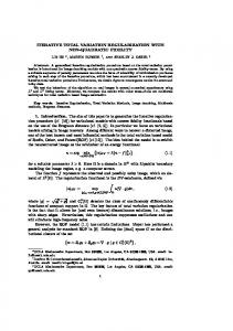
Figure 1. Depicting the three typical problems of current stateof-the-art flow estimate techniques: Untextured ares, small image details and occlusions. First column shows cropped input images; second (first and second row) the ground truth result; the third the estimated flow using a classical total variation-like regularity; the last column shows the result of our proposed method. (Datasets: Teddy, Mequon and Backyard)

of a variational motion estimation model is given by the minimization problem n o min R(u) + D(I0 , I1 , u) , u

(1)

with the unknown motion field u = (u1 , u2 )T : Ω → R2 and the input images I0 and I1 , all defined on the image domain Ω ⊂ R2 . The motion fields smoothness is ensured by the regularization term R(u), which typically penalizes first of higher order derivatives using e.g. quadratic [10] or robust [4] potential functions. The term D(u) is the data term which measures the similarity of the input images for a given motion field. Commonly used similarity measures are based on image intensities [29], derivatives of image intensities [5] or more sophisticated similarity measures [18]. Total variation-like regularization has been proposed by Shulman et al. in [17] in order to allow for dis-

continuities in the motion field1 , while still being a convex function. In subsequent work [1, 2, 5, 25, 29], the authors proposed to minimize slight variants of the following energy functional Z nZ o min |∇u1 | + |∇u2 | dx + λ |ρ(x)| dx (2) u

Ω

Ω

which consists of total variation (TV) regularization of the motion field and a robust L1 data term to penalize deviations in the image similarity term. The free parameter λ is used to define the tradeoff between regularization and data fitting. For minimization, one needs to linearize the image residual ρ(x) = I0 (x) − I1 (x + u(x)) at a given point u0 (x) = (u10 , u20 )T , which leads to the classical optical flow equation ρ(x) ≈ It (x) + (∇I1 (x))T (u(x) − u0 (x)), where It (x) = I0 (x)−I1 (x+u0 (x)) denotes the temporal derivative. In [5] Brox et al. postpone the linearization of the image residual to the numerical algorithm. After linearization, energy (2) yields a convex optimization problem which can be solved using for example the primal-dual quadratic splitting technique of [29]. Unfortunately, the linearization of the image residual has the disadvantage, that the model is only valid in a small proximity of u0 . In order to account for larger motion, the entire approach has to be integrated into a coarse-to-fine warping framework [8]. This, however, makes the overall approach again non-convex. Besides the problem of non-convexity, state-of-the art motion estimation algorithms mainly suffer from three major problems (cf . Figure 1): • Untextured regions: In poorly textured regions, no matching can be performed and hence strong regularization is needed to propagate the motion from textured regions into the untextured areas.

These approaches suffer from taking only a small neighborhood into account. Hence, an expanded proximal influence allows to compute adaptive support weights between the neighboring pixels to further strengthen their cohesion. Such pixel groupings have already been considered in the field of image restoration and stereo matching: When performing image restoration, the support weights are computed based on the fact that natural images exhibit a large amount of redundancy. This leads to the well known neighborhood filters [7, 20, 27] which belong to best performing methods. A variational interpretation of these ideas lead to non-local regularizers [6, 9] with similarly computed proximal relations. In the context of stereo matching, Yoon and Kweon [28] computed adaptive support weights to locally adapt the local matching window to the image structure which leads to a significant improvement of the method. Interestingly, for motion estimation, this powerful principle has been neglected so far. We are aware of only one work which goes into this direction. In [26] Xiao et al. proposed to incorporate the bilateral Gaussian filter into a variational motion estimation framework in order to improve the performance in occluded regions. In this paper we propose a unified variational framework to cope with the problems we have identified above. Our method is based on non-local total variation regularization which allows us to incorporate a low level segmentation process into the variational model. Furthermore, contrary to most existing approaches which rely on the linearized brightness constancy assumption (often referred to as optical flow equation), we propose to perform a second order Taylor expansion of the data term which allows us to use more sophisticated data terms such as the normalized cross correlation.

2. Non-Local Total Variation Regularization • Occlusions: As soon as motion is present in the images, regions are occluded or exposed by moving objects. Those occluded regions cannot be matched between the image frames. • Small Scale Structures: Small scale structures with a relative large movement are hard to preserve in the motion field since isotropic regularization does not adapt well to the local image structure. Most approaches trying to address these problems are based on image driven regularizers [11, 23, 25], advanced smoothness assumptions [21] or statistical learning [15, 19]2 . 1 Interestingly, the work of Shulman et al. has been published several years before total variation methods were popularized by Rudin Osher and Fatemi [16] for image denoising. 2 According to [12] we point out that it is not relevant to learn accurate statistical models, as long as simple MAP estimation is used to infer the most likely solution.

Considering the movement of a single object, it is likely that part of the object delineate a similar motion pattern. We utilize the coherence of neighboring pixels to enforce the same kinesic behavior and strengthen the regularization within these linked areas and reduce its influence across area boundaries. The idea of non-local total variation (NLTV) regularization incorporates this information directly into the regularization energy yielding Z Z R(u) = Ω

Ω

w(x, y) |u1 (x) − u1 (y)|ε +
|u2 (x) − u2 (y)|ε dy dx , (3)

where |q|ε denotes the Huber norm given by ( 2 |q| |q| ≤ ε . |q| = 2ε ε |q| − 2 else

(4)

(a)

to fulfill the well-known brightness constancy constraint. Any changes in the illumination within the scene violate this assumption which cause methods based on this constraint to fail. Classical approaches often introduce a pre-processing step to reduce influence of illumination changes using for example a structure-texture decomposition of the input images [24]. In terms of image matching it is well established that the normalized cross correlation is invariant to multiplicative illumination changes which could be useful in the field of motion estimation too. Consider the image matching energy Z D(I0 , I1 , u) = λ δ(x, u(x)) dx , (6)

(b)

Ω

where δ(x, u(x)) is the pointwise data term depicting the truncated normalized cross correlation (TNCC). Therefore we introduce the mean of a certain patch by Z µ0 (x) = I0 (y)BΣ (x − y) dy and (7) ZΩ µ1 (x) = Ie1 (y)BΣ (x − y) dy , (8) Ω

(c)

(d)

Figure 2. Proximal weight (b), color-similarity weight (c) and combined weight (d) for the marked region (a) in the Army dataset.

The parameter ε is a small constant which defines the threshold between quadratic and linear penalization of the variations. The advantage of the Huber norm over the pure total variation is avoiding the preference of piecewise constant motion fields [25]. The function w(x, y) is a weighting function which is used to define the mutual support between the pixels at positions x and y. Based on the idea of Yoon and Kweon [28] we compute the support-weights based on color-similarities and on spatial distances: w(x, y) = e−(

∆c (x,y) ∆ (x,y) + sβ α

)

(5)

Here ∆c (x, y) denotes the color similarity between I0 (x) and I0 (y) measured as Euclidean distance in the Lab color space and ∆s (x, y) is the Euclidean distance, i.e. the proximity between x and y. The parameters α and β are used to tune the influence of color similarity and spatial proximity. Figure 2 shows an exemplary patch of the Army dataset showing the spatial and color support weights. From this it becomes clear that the support weights essentially encode a low level segmentation into the regularization framework.

3. Second Order Approximation of the Data Term Standard optical flow estimation techniques using a formulation like (2) utilize a linearization of the image residual

R where BΣ denotes a box filter of width Σ and B(z) dz = 1 and Ie1 (y) = I1 (y + u0 ) the warped image. Likewise the standard deviation σ(x) is defined as sZ 2 (I(y) − µ(x)) BΣ (x − y) dy . (9) σ0,1 (x) = Ω

Hence the image matching energy can be defined as NCC(x, u(x)) =

1 · σ0 (x)σ1 (x)

Z (I0 (y) − µ0 (x))(Ie1 (y) − µ1 (x))BΣ (x − y) dy . (10) Ω

Note that the matching term is computed based on the warped image Ie1 (x) = I1 (x + u0 ) to account for the local distortion within the correlation window. This stands in contrast to [18] which assumes that the motion remains constant within the correlation window. Furthermore, to gain robustness against occlusions we disregard negative correlations and therefore call the NCC truncated (TNCC): n o δ(x, u(x)) = min 1, 1 − NCC(x, u(x)) (11) Using such a data fidelity measure, the classical approach of linearizing the image function is no longer tractable since the TNCC depicts a highly non-linear function. We therefore propose to perform a direct second-order Taylor expansion of the pointwise data term, yielding δ(x, u(x)) ≈ δ(x, u0 (x))+ T

(∇δ(x, u0 (x))) (u(x) − u0 (x)) +
T (u(x) − u0 (x)) ∇2 δ(x, u0 (x)) (u(x) − u0 (x)) , (12)

where ∇2 δ(x, u0 (x)) denotes a positive semi-definite approximation of the Hessian matrix   + (δxx (x, u0 (x))) 0 , (13) ∇2 δ = + 0 (δyy (x, u0 (x))) where we only allow for positive second order derivatives to ensure convexity of the second order approximation and have neglected mixed derivatives. Hence the data term is by construction convex which will enable us to apply efficient primal-dual optimization schemes. In a numerical implementation we use simple finite differences approximations to compute the spatial derivatives of δ(x, u(x).

usage of duality principles [14] provide faster convergence rates and are therefore preferable. In addition the primaldual algorithm enables easier implementations which can be rather easily parallelized utilizing modern graphics hardware and optionally speed up the calculations. However, since (15) is convex in u we actually can make use of duality principles to arrive at the following compact saddle point formulation n o min max h(Ah uh )i,j,k,l , (ph )i,j,k,l i+G(uh )−F ∗ (ph ) , uh

ph

(16) where the linear operator Ah assembles the neighborhood relations defined through the non-local operator

4. Minimization

(Ah uh )i,j,k,l = uhi,j − uhk,l

Putting together the regularization term (3) and the data term (6) we arrive at the following optimization problem nZ Z min w(x, y) |u1 (x) − u1 (y)|ε u Ω Ω
+ |u2 (x) − u2 (y)|ε dy dx Z T (14) +λ (∇δ(u0 (x))) (u(x) − u0 (x)) T

+ (u(x) − u0 (x)) o
∇2 δ(u0 (x)) (u(x) − u0 (x)) dx . In order to optimize (14) we define a vector space U h = R2N M on a Cartesian grid Ωh = {(ih, jh) : 1 ≤ i ≤ N, 1 ≤ j ≤ M } with the spacing h, a discretized motion vector uh = (uh1 , uh2 )T ∈ U h and a discrete weighting between the pixels (i, j) and (k, l) denoted as (wh )i,j,k,l . We then introduce the following discrete version of (14) nX X min (wh )i,j,k,l (uh )i,j − (uh )k,l i,j k,l∈Ni,j

+ λ

X

and (ph )i,j,k,l = ((ph1 ), (ph2 ))Ti,j,k,l is the dual variable defined on the vector space P h = R2N M |N | , where |N | is the size of the neighborhood. The function G(uh ) is given by G(uh ) = λ

X


T
∇h δ(uh0 ) i,j (uh )i,j − (uh0 )i,j

i,j


T + (uh )i,j − (uh0 )i,j

∇2,h δ(uh0 ) i,j (uh )i,j − (uh0 )i,j (18)

Ω

uh

(17)


T
∇h δ(uh0 ) i,j (uh )i,j − (uh0 )i,j

i,j


T + (uh )i,j − (uh0 )i,j

o ∇2,h δ(uh0 ) i,j (uh )i,j − (uh0 )i,j , (15) where Ni,j defines a set of pixels used by the non-local operator at the current pixel (i, j). The first order derivatives ∇h δ(uh0 ) and second order derivatives ∇2,h δ(uh0 ) are computed using standard central differences on the discrete lattice. Due to the L1 norm, optimization of this energy is not a trivial task. While the lagged diffusivity algorithm, introduced by Vogel and Oman [22], converges rather slow, the

and F ∗ (ph ) is obtained by computing the Legendre-Fenchel transformation with respect to the Huber function (4) and is given by ε 2 (19) F ∗ (ph ) = ph + IK , 2 where IK denotes the so-called indicator function for the convex set K given by I = 0 if ph ∈ K and ∞ otherwise. The convex set K is given by n K = ph = (ph1 , ph2 )T : |(ph1 )i,j,k,l | ≤ (wh )i,j,k,l , |(ph2 )i,j,k,l | ≤ (wh )i,j,k,l o ∀ i, j, k, l ∈ Ωh × Ωh .

(20)

To obtain a solution we apply the convergent primal-dual algorithm recently proposed in [13]. The iterates are given by 
−1 h n+1  = (I + τd ∂F ∗ ) (ph )n + τd A(uh )n (p )
−1 (uh )n+1 = (I + τp ∂G) (uh )n − τp AT (ph )n+1   h n+1 (u ) = 2(uh )n+1 − (uh )n , (21) where τp and τd are the primal and dual step sizes satisfying −1 τp τd ≤ kAh k2 . (I + τd ∂F ∗ ) denotes the resolvent func∗ h tion with respect to F (p ) which is given as the minimizer

of ( (ph )n+1 = arg min ph

h n+ 21 2

h

kp − (p ) 2τd

k

) + F ∗ (ph )

.

(22) The solution of this minimization problem is given by h n+1 pn+1 , (ph2 )n+1 )Ti,j,k,l , where i,j,k,l = ((p1 )   (ph1,2 )n+1 i,j,k,l =

n+ 1

2 (x) (ph1,2 )i,j,k,l

h wi,j,k,l



1 + ετd

,

(23)

this paper we use a scale factor of 0.8 to construct the image pyramid. Performing the iterative optimization (21) we perform 5 warps with 100 iterations per level. We implemented the proposed motion estimation approach in Matlab and additionally in C++ on the GPU utilizing the Nvidia CUDA framework. Such variational formulations match the parallelization capabilities of modern GPUs well and enable such complex computations like the big neighborhood relations in a reasonable time vastly outperforming the Matlab implementation.

h −wi,j,k,l

and [q]ba denotes the pointwise truncation of q to the inter−1 val [a, b]. The function (I + τp ∂G) denotes the resolvent h function with respect to G(u ) which is given as the minimizer of ( ) 1 kuh − (uh )n+ 2 k2 h n+1 h (u ) = arg min + G(u ) . 2τp uh (24) This is a simple pointwise quadratic optimization problem whose pointwise solutions yield (uhi,j )n+1 = ((uh1 )n+1 , (uh2 )n+1 )Ti,j , where  (uh1 )n+1 = (δxx (uh1,0 ))i,j (uh1,0 )i,j − i,j  1 1 (δx (uh1,0 ))i,j + ((uh1 )i,j )n+ 2 (25) τp 1 , (δxx (uh1,0 ))i,j + τ1p and  h h (uh2 )n+1 i,j = (δyy (u2,0 ))i,j (u2,0 )i,j − (δy (uh2,0 ))i,j + 1 (δyy (uh2,0 ))i,j +

 1 1 ((uh2 )i,j )n+ 2 τp

1 τp

(26)

.

4.1. Implementation In order to apply the discretized linear operator Ah from (16), assembling the non-local operators neighborhood relations, we restrict the diameter of the corresponding window N to dN = 2β +1. Due to the fact that the proximity portion of the weights (5) suppress the influence of the color similarities at a certain distance, no essential information is lost when clipping the window of linear operator A. This influence of the support weights on the window size can be shown in Figure 2(b) where the proximal support vanishes when approaching the window border. As mentioned in the introduction, local methods of motion estimation are not able to cope with large displacements and therefore we embed our approach into a coarseto-fine/warping approach. For all presented experiments in

5. Results To emphasize the potential of our approach we did some evaluations on the already introduced Middlebury benchmark database [3] and achieve top rankings for a lot of the evaluated metrics (cf . http://vision. middlebury.edu/flow). According the ‘average endpoint error’ (AEPE) and the ‘average angular error’ (AAE) we rank second and fourth at the time of publication (cf . Figure 4). As requested the results were submitted with a constant set of parameters. In fact all of our results throughout this paper were produced with the same parameter set as well. In order to obtain a reasonable parameter set for a variety of different input data we did an evaluation on how the results change when adapting the weighting function (5) with changing its parameters α and β. For this evaluation we utilize the training dataset of the Middlebury benchmark site and its given ground truth results. Therefore we can calculate the error metrics for changing parameters. Figure 3 shows the mean of the error metrics (AAE and AEPE) over the complete dataset for a varying α and β. Changing the parameter β adapts the spatial influence of the weight by changing the proximal influence. As β increases the considered window for applying non-local regularization grows. Regarding the error metrics, the AAE and AEPE drop significantly with an decrease of β up to a value of β ≈ 4. For values of 3 ≤ β ≤ 8 the error remain quite constant and for a β ≥ 8 the calculated errors increase again. Interpreting this evaluation enforces the idea on grouping regions together up to a certain extend. A large spatial influence, meaning grouping rather big regions together, pushes big areas towards similar motion. Considering a deformable or even a simple rotating object, a too big spatial influence of the regularization forces the motion to be similar and causes oversmoothed results and therefore an increase in the error metrics as presented in the plot in Figure 3(a). With respect to α the result is similar (cf . Figure 3(b)). The parameter α is responsible to enforce color similarities when calculating weights for the non-local regularization. In case of α, a low value means that only the resultant color groupints are considered for weight calculations whereas for increasing α proximal weights are taken into

Dataset: TV-L1 : NL-TV-L1 : TV-TNCC: NL-TV-TNCC:

Dimetrodon 0.27 0.24 0.20 0.16

Hydrangea 0.22 0.26 0.19 0.15

RubberWhale 0.18 0.21 0.12 0.08

Venus 0.39 0.35 0.33 0.29

Grove 2 0.20 0.24 0.20 0.14

Grove 3 0.71 0.69 0.70 0.54

Urban 2 0.48 0.45 0.46 0.35

Urban 3 0.74 0.57 0.57 0.43

Table 1. Separate evaluation of regularization and data term (only AEPE given). Each row represents a combination of either TV or non-local regularization in combination with classical pointwise L1 data term or the proposed TNCC method.

TV-L1 0.40

0.32

4.75

AAE AEPE

4.5

3.75

AEPE

AAE

0.28

4

0.26

3.5 2

4

6

8

10 β

12

14

16

18

(a) 4.5

0.4 AAE AEPE

AEPE

AAE

0.34 3.75 0.32 3.5

0.3

3.25

0.28 6

8

10

To conclude this evaluation we set α = 5, β = 5, λ = 2 and ε = 1.5 for all of our evaluations and obtain very stable results for all sort of datasets. For this parameter settings and the aforementioned implementation details (cf . Section 4.1) our CUDA implementation takes 15 seconds on the Urban sequence on a recent 64bit Linux system, equipped with an Nvidia GTX 280. For completeness, we also give an overview of the color-coded results on the Middlebury training and test set in Figure 5 and 6.

6. Conclusion and Future Work

0.36 4

4

NL-TV-TNCC 0.27

0.38

4.25

2

TV-TNCC 0.35

Table 2. Mean AEPE over all datasets in Table 1.

0.3 4.25

NL-TV-L1 0.38

12

α

(b)

Figure 3. Evaluation of varying (a) spatial influence β and (b) color similarity weights α; mean values of AAE and AEPE evaluating all sequences from the Middlebury training database;

account too. Again the calculated AAE and AEPE drop up to a certain extend when increasing α up to a value of ≈ 3. Then the metrics remain stable up to α ≈ 8 and increase slightly for larger values. The result shows that solely relying on segmentation does not reach as good accuracy as taking a mixture of color similarity and proximal weighting into account. In this paper we introduced two improvements over the classical TV-L1 motion estimation method. To give a separate evaluation for both parts, the regularization and the data term, we combined all possible combinations to judge the contribution of the single parts respectively. In Table 1 and 5 the non-local regularization and the TNCC data fitting is added one at a time to a TV-L1 method. The results shows that the best results can be obtained when combining both proposed parts presented in this paper.

In this paper we illustrated the benefit of a non-local total variation like regularization and a robust data term in combination with a versatile optimization method embedded into a variational formulation. The proposed method can cope with major problems that affect the widely used motion estimation techniques based on TV regularities and L1 data term like poorly textured areas, occlusions and small image structures. Although we can tackle many of diverse problems with our approach, handling big disparities still remains a unsolved issue using such local approaches. To enable the estimation of large object movements the method has to be implemented within coarse-to-fine approach with all its related drawbacks. Although we investigated work on optimizing the creation process of the image pyramids it may occur that small details are cleared on coarser levels due to oversmoothing. Therefore we will concentrate our further work on estimating large disparities. We have great promise on boosting the accuracy of motion estimation using the proposed method of this paper without the necessity on using typical coarse-to-fine approaches.

References [1] A.Bruhn, J.Weickert, and C.Schn¨orr. Lucas/Kanade meets Horn/Schunck: Combining local and global optic flow methods. Int’l J. Computer Vision, 61(3):211–231, 2005. 2 [2] G. Aubert, R. Deriche, and P. Kornprobst. Computing optical flow via variational techniques. SIAM J. Appl. Math., 60(1):156–182, 1999. 2

Figure 4. Screenshot of the Middlebury benchmark results (http://vision.middlebury.edu/flow). The proposed method is denoted as NL-TV-NCC.

(a) Dimetrodon (0.16/3.21)

(e) RubberWhale (0.08/2.55)

(b) Grove2 (0.14/1.94)

(f) Urban2 (0.35/2.92)

(c) Grove3 (0.54/6.05)

(g) Urban3 (0.43/3.36)

(d) Hydrangea (0.15/1.90)

(h) Venus (0.29/4.27)

Figure 5. Flow results on the training sequences of the Middlebury benchmark dataset. The respective AEPE and AAE are given in brackets (AEPE/AAE).

[3] S. Baker, D. Scharstein, J. P. Lewis, S. Roth, M. J. Black, and R. Szeliski. A database and evaluation methodology for optical flow. In ICCV, 2007. 1, 5 [4] M. J. Black and P. Anandan. Robust dynamic motion estimation over time. pages 296–302, June 1991. 1 [5] T. Brox, A. Bruhn, N. Papenberg, and J. Weickert. High accuracy optical flow estimation based on a theory for warping. In ECCV, pages 25–36, 2004. 1, 2 [6] T. Brox, O. Kleinschmidt, and D. Cremers. Efficient nonlocal means for denoising of textural patterns. IEEE Trans. on Image Processing, 17(7):1083–1092, July 2008. 2 [7] A. Buades, B. Coll, and J.-M. Morel. Nonlocal image and movie denoising. International Journal of Computer Vision,

76(2):123–139, 2007. 2 [8] D. J. Fleet and Y. Weiss. Optical flow estimation. In N. Paragios, Y. Chen, and O. Faugeras, editors, Handbook of Mathematical Models in Computer Vision, chapter 15, pages 239– 258. Springer, 2006. 2 [9] G. Gilboa and S. J. Osher. Nonlocal operators with applications to image processing. Technical report, UCLA CAM Report 07-23, July 2007. 2 [10] B. K. P. Horn and B. G. Schunck. Determining optical flow. Artificial Intelligence, 17:185–203, 1981. 1 [11] H.-H. Nagel and W. Enkelmann. An investigation of smoothness constraints for the estimation of displacement vector fields from image sequences. IEEE Trans. on Pattern Analy-

Figure 6. Flow results on the test sequences of the Middlebury benchmark dataset.

sis and Machine Intelligence, 8(5):565–593, 1986. 2 [12] M. Nikolova. Model distortions in bayesian map reconstruction. Inverse Problems and Imaging, (2):399–422, 2007. 2 [13] T. Pock, D. Cremers, H. Bischof, and A. Chambolle. An algorithm for minimizing the mumford-shah functional. In ICCV, 2009. 4 [14] R. T. Rockafellar. Convex analysis. Princeton Landmarks in Mathematics. Princeton University Press, Princeton, NJ, 1997. Reprint of the 1970 original, Princeton Paperbacks. 4 [15] S. Roth and M. J. Black. On the spatial statistics of optical flow. IJCV, 74(1):33–50, August 2007. 2 [16] L. Rudin, S. J. Osher, and E. Fatemi. Nonlinear total variation based noise removal algorithms. Physica D, 60:259– 268, 1992. 2 [17] D. Shulman and J.-Y. Herv´e. Regularization of discontinuous flow fields. In Proceedings Workshop on Visual Motion, pages 81–86, 1989. 1 [18] F. Steinbruecker, T. Pock, and D. Cremers. Advanced data terms for variational optic flow estimation. In Vision, Modeling, and Visualization Workshop, Braunschweig, Germany, 2009. 1, 3 [19] D. Q. Sun, S. Roth, J. P. Lewis, and M. J. Black. Learning optical flow. In ECCV, volume III, pages 83–97, 2008. 2 [20] C. Tomasi and R. Manduchi. Bilateral filtering for gray and color images. In ICCV, pages 839–846, 1998. 2 [21] W. Trobin, T. Pock, D. Cremers, and H. Bischof. An unbiased second-order prior for high-accuracy motion estimation. In Pattern Recognition, DAGM 2008, 2008. 2

[22] C. Vogel and M. Oman. Iteration methods for total variation denoising. SIAM J. Sci. Comp., 17:227–238, 1996. 4 [23] A. Wedel, D. Cremers, T. Pock, and H. Bischof. Structureand motion-adaptive regularization for high accuracy optic flow. In ICCV, Kyoto, Japan, 2009. 2 [24] A. Wedel, T. Pock, C. Zach, D. Cremers, and H. Bischof. An improved algorithm for TV-L1 optical flow. In Proceedings of the Dagstuhl Motion Workshop, September 2008. 3 [25] M. Werlberger, W. Trobin, T. Pock, A. Wedel, D. Cremers, and H. Bischof. Anisotropic Huber-L1 optical flow. In BMVC, London, UK, September 2009. 2, 3 [26] J. Xiao, H. Cheng, H. Sawhney, C. Rao, and M. Isnardi. Bilateral filtering-based optical flow estimation with occlusion detection. In ECCV, volume I, pages 211–224, 2006. 2 [27] L. P. Yaroslavsky. Digital Picture Processing — an Introduction. Springer, Berlin, 1985. 2 [28] K.-J. Yoon and I. S. Kweon. Adaptive support-weight approach for correspondence search. IEEE Trans. on Pattern Analysis and Machine Intelligence, 28(4):650–656, 2006. 2, 3 [29] C. Zach, T. Pock, and H. Bischof. A duality based approach for realtime TV-L1 optical flow. In Pattern Recognition, DAGM, pages 214–223, 2007. 1, 2