and Nj. A linear equation that specifies the desired relative position between vi and vj in the de- formed mesh can be formulated as xi xj = c1 jibj. 1 +c2 jibj. 2 +c3.
To appear in ACM Transactions on Graphics (Special Issue of SIGGRAPH 2006)
A Fast Multigrid Algorithm for Mesh Deformation Lin Shi
Yizhou Yu
Nathan Bell
Wei-Wen Feng
University of Illinois at Urbana-Champaign
Figure 1: The idle CAMEL becomes a boxer with the help of MOCAP data and our mesh deformation system.
Abstract
can be handle positions, key frames or silhouettes, and the editing system automatically solves a sparse system of equations to satisfy these constraints. Nevertheless, a serious problem that still hampers the deployment of this type of techniques is their scalability. When meshes become large and complex, the performance of the numerical solver becomes the bottleneck of the entire system. While solutions to cope with this problem exist – including small regions of interest (ROI) and precomputed matrix factorizations – they restrict the scope of editing operations. The multigrid method on the other hand has the potential to solve large-scale sparse systems efficiently without a significant setup time. While the user most often only needs to pick up a handle to manipulate a mesh, it is sometimes necessary to define and manipulate new handles that have not been preprocessed. Furthermore, in a general mesh editing environment, mesh deformation needs to be mixed with other mesh editing operations, such as remeshing and merging. This is evidenced by routine practice in game development where large-scale meshes are edited first before simplified to a size suitable for real-time rendering. Some of these editing operations result in an altered system of linear equations that need to be solved on the fly. When the mesh is large, a fast multigrid algorithm can solve the altered linear system in a less stressful way than the factorization stage in direct solvers. In this paper, we introduce a fast multigrid technique tailored for mesh deformation to support the aforementioned scenario. Although the multigrid method has become a popular choice for largescale mesh processing [Ray and Levy 2003; Aksoylu et al. 2005], there are still a number of challenges we need to overcome to achieve acceptable interactive performance. First, recent mesh deformation techniques often have two passes with the first pass solving for local frames and the second pass solving for vertex coordinates. How can we effectively reformulate these passes so that they become more compatible with multigrid solvers? Second, the multigrid method requires a hierarchical structure and must accommodate user-provided deformation constraints within this hierarchy. How can we properly handle these aspects? Third, when moving between grid levels the multigrid method applies a pair of prolongation and restriction operators. How should we design such operators to speed convergence? We have developed effective techniques to overcome these challenges. First, we revise the formulations for mesh deformation so that they can be adequately solved by local relaxations. In partic-
In this paper, we present a multigrid technique for efficiently deforming large surface and volume meshes. We show that a previous least-squares formulation for distortion minimization reduces to a Laplacian system on a general graph structure for which we derive an analytic expression. We then describe an efficient multigrid algorithm for solving the relevant equations. Here we develop novel prolongation and restriction operators used in the multigrid cycles. Combined with a simple but effective graph coarsening strategy, our algorithm can outperform other multigrid solvers and the factorization stage of direct solvers in both time and memory costs for large meshes. It is demonstrated that our solver can trade off accuracy for speed to achieve greater interactivity, which is attractive for manipulating large meshes. Our multigrid solver is particularly well suited for a mesh editing environment which does not permit extensive precomputation. Experimental evidence of these advantages is provided on a number of meshes with a wide range of size. With our mesh deformation solver, we also successfully demonstrate that visually appealing mesh animations can be generated from both motion capture data and a single base mesh even when they are inconsistent. CR Categories: I.3.5 [Computer Graphics]: Computational Geometry and Object Modeling—Boundary representations Keywords: Mesh Editing, Laplacian, Constraints, Graph Hierarchy, Prolongation/Restriction Operators
1
Introduction
Surface-based mesh editing has received much attention recently due to its capability to produce visually appealing results while at the same time making the underlying numerical computation transparent to the user. The user only needs to specify the goals, which
1
To appear in ACM Transactions on Graphics (Special Issue of SIGGRAPH 2006)
2
ular, we analytically obtain a closed-form formulation for the optimization of vertex coordinates, thereby avoiding expensive sparse matrix multiplications. Second, we quickly create a hierarchy using a simple graph coarsening technique that ignores the initial mesh structure. Boundary conditions are not explicitly considered during the construction of the hierarchy. Instead, they are incorporated algebraically in the equations and in the prolongation/restriction operators. Most importantly, we develop a novel technique that automatically obtains prolongation and restriction operators using a weighted graph perspective. These operators better maintain the consistency of equations among different levels, and thus significantly improve the convergence rate. As a result, our algorithm can outperform existing multigrid solvers and the factorization stage of direct solvers. We demonstrate the advantages and utility of these features in complex mesh editing examples.
Basic Formulations
Here we describe the basic formulations we adopt for mesh deformation. Note that these formulations can be applied to surface triangle meshes with or without a volume graph [Zhou et al. 2005]. In practice, we most often construct such a graph to have better volume preservation. Following [Lipman et al. 2005], an initial local frame is defined at each vertex of the graph. The orientation of the local frame can be arbitrary. Given a set of rotation, scaling and/or translation constraints, we still formulate mesh deformation as a two-pass process. During the first pass, we first compute harmonic guidance fields over the mesh as in [Zayer et al. 2005], and then obtain modified orientation and scale of the local frame at every unconstrained vertex by interpolating relevant constraints using the harmonic guidance fields. The modified orientation and scale are then fixed at all vertices during the second pass and the coordinates of every unconstrained vertex are solved as in [Lipman et al. 2005]. More details follow.
1.1 Related Work There have been many approaches for mesh modeling and editing. In the following, we will focus on geometry-based mesh deformation techniques only. Physically based deformation based on elasticity models is beyond the scope of this paper. FFD techniques [Sederberg and Parry 1986] need to embed a surface mesh inside a volume lattice. It is hard to precisely control the surface deformation results using FFD because it is achieved indirectly by manipulating the lattice points. Recent work [Botsch and Kobbelt 2005] has replaced the lattice with volume-based radial basis functions (RBFs) which further induce deformation on the target mesh surface. Impressive performance on large meshes has been achieved for deformations with predefined handles. Flexible mesh modeling and deformation can be achieved by employing a multiresolution decomposition of the original mesh [Zorin et al. 1997; Kobbelt et al. 1998; Guskov et al. 1999]. By choosing to work at an appropriate resolution, one can manipulate or edit the mesh at a desired scale to reduce the amount of manual effort. Recently, surface-based mesh editing techniques [Alexa 2003; Sorkine et al. 2004; Yu et al. 2004; Lipman et al. 2005; Zayer et al. 2005] demonstrate that it is possible to achieve similar results without exposing the multiresolution structure of the mesh. The user directly manipulates the mesh surface at its finest level and the scale of manipulation is controlled by a region of interest. High frequency mesh details can be well preserved by locally or globally supported deformation fields which only modify the low frequency part of the mesh geometry. At the core of a surface-based mesh editing system lies a mesh representation based on differential coordinates, such as Laplacian or gradient coordinates. Such systems typically manipulate the differential coordinates of the undeformed mesh first, followed by a reconstruction of the deformed mesh from the modified differential coordinates. Most techniques in this category have two passes with the first pass addressing rotation and scaling, and the second pass reconstructing vertex coordinates. While the second pass is commonly formulated as a least-squares minimization, various techniques have been proposed for the first pass, including geodesic distance based propagation [Yu et al. 2004], harmonic field based interpolation [Zayer et al. 2005], and least-squares minimization based on a rotation-invariant representation [Lipman et al. 2005]. In [Zhou et al. 2005], a volume graph is constructed at the interior of a closed mesh to prevent volume loss during excessive bending and twisting. Mesh deformation is also closely related to shape interpolation which involves more than one originally undeformed key shapes. An effective shape interpolation technique for simplicial complexes was introduced in [Alexa et al. 2000]. This technique has been generalized to surface-based deformation transfer in [Sumner and Popovi´c 2004] and nonlinear interpolation among multiple key shapes in [Sumner et al. 2005].
2.1 The First Pass During the first pass, the goal is to smoothly ”interpolate” both rotation and scaling constraints over the entire mesh surface. We perform interpolation for these two types of constraints separately because the orthogonality of local frames requires that rotation interpolation still produce valid rigid body rotations. The interpolation of scaling constraints is performed by computing a single scalar harmonic field, which is the solution of the Laplace equation, ∆ν � 0�
(1)
over the mesh surface with the scaling constraints as boundary conditions. The discretization of this Laplace equation gives rise to a sparse linear system. As we know, a harmonic field is the equilibrium state of a diffusion process. Ideally, one should generalize this observation from scaling constraints to rotation constraints each of which can be represented as a unit quaternion. We define an orientation diffusion process as follows, ∂q � ∆O q� (2) ∂t where ∆O represents a generalized Laplacian operator for orientations. Since a discrete Laplacian operator at a mesh vertex returns a linear combination of the values of a quantity within the 1-ring neighborhood of the vertex, such a Laplacian operator can be easily generalized to orientations because any linear combination of unit quaternions is well defined as long as the participating quaternions follow a predefined order and the weights form a partition of unity. Iteratively simulating such an orientation diffusion process as defined in (2) with appropriate boundary conditions leads to a smooth quaternion field over the mesh. Each iteration of the simulation is a local relaxation. The resulting quaternion field can then be applied to the local frame at every vertex to obtain the modified local frame. However, orientation diffusion using quaternions is still more expensive than scalar diffusion. In practice, we adopt one of the schemes presented in [Zayer et al. 2005] which computes a distinct bounded scalar harmonic field for each and every rotation constraint. Each of the bounded harmonic fields is computed using a unique set of boundary conditions which set one at the vertices sharing the same rotation constraint being considered while zero at the vertices with the rest of the rotation constraints. The value of the resulting harmonic field at an unconstrained vertex serves as the interpolation coefficient for the rotation constraint being considered. The final rotation at that vertex is interpolated from all rotation constraints using the computed coefficients. Such an interpolated rotation is a good approximation of the rotation obtained from orientation diffusion.
2
To appear in ACM Transactions on Graphics (Special Issue of SIGGRAPH 2006) 2.2 The Second Pass Our formulation for solving modified vertex coordinates in the deformed mesh is based on the method in [Lipman et al. 2005]. Suppose vertex v j belongs to vertex vi ’s 1-ring neighborhood. The coordinates of vi and v j are denoted as xi and x j . The modified local frame at v j has three axes, b1j , b2j and N j . A linear equation that specifies the desired relative position between vi and v j in the deformed mesh can be formulated as xi � x j � c1ji b1j � c2ji b2j � c3ji N j �
Figure 2: Orientation diffusion (left) and harmonic fields (center) produce more natural deformations than the method in [Lipman et al. 2005]. Two constrained handles are located at the two ends of the mesh structure.
(3)
where c1ji , c2ji and c3ji are scalar coefficients encoding the relative position of vi with respect to the local frame at v j in the original undeformed mesh. If we switch the roles of xi and x j in (3), we can obtain a second equation for the same vertices as follows, x j � xi � c1i j bi1 � c2i j bi2 � c3i j Ni �
(4) Figure 3: A SPRING is deformed using a spatial deformation technique (center) and our method (right). In the spatial case, points in close proximity (Euclidean metric) move together even when their geodesic distance is much larger. In contrast, our mesh-based approach contains this geodesic information implicitly.
Subtracting (4) from (3), we have xi � x j
� d ji
(5)
�
where
� � �� 1 �� 1 j c ji b1 � c2ji b2j � c3ji N j � c1i j bi1 � c2i j bi2 � c3i j Ni � 2 (6) Since there is such a linear equation for every pair of connected vertices, a least-squares solution can be sought for all the vertex coordinates in the deformed mesh. Using a matrix multiplication to obtain the normal equations of this least-squares minimization is actually a very costly step. Fortunately, in this particular case, it is straightforward to obtain the normal equations analytically. From a different perspective, (5) can be viewed as an equation that provides a prediction of vi ’s location using the coordinates and local frame at v j . Suppose vi ’s 1-ring neighbors are indexed by N �i�. Obviously, there are �N �i�� potentially conflicting predictions like this for vi . Suppose the edge between vi and v j is associated with a weight wi j and wi j � w ji . The (weighted) least-squares solution of vi ’s coordinates should be the (weighted) average of the �N �i�� predictions. Therefore, the system of normal equations must contain exactly one equation like the following for every vertex. d ji �
xi �
∑ j¾N �i� w ji x j ∑ j¾N �i� w ji
�
∑ j¾N �i� w ji d ji ∑ j¾N �i� w ji
�
on edges, it can be used for deforming any graph structures, not just triangle meshes. Therefore, it is more general than the discretized Poisson equation adopted in [Yu et al. 2004] which was tailored for triangle meshes. Our formulation is also different from the one used in Laplacian mesh editing [Sorkine et al. 2004] which solves a bi-harmonic system.
2.3 Discussion We have performed two simple tests to justify the choices we made here. Fig. 2 shows a comparison of three deformation results. We use the same linear system in (8) as the second pass in all three tests. The first pass adopts three different techniques including orientation diffusion, bounded harmonic fields [Zayer et al. 2005], and the linear system in [Lipman et al. 2005]. The results from the first two are extremely close and distribute both twisting and bending more uniformly across the surface than the third approach which tends to concentrate deformation halfway between the two handles. This is because the method in [Lipman et al. 2005] does not enforce the orthogonality of the modified local frames. In another simple test shown in Fig. 3, we compare a space deformation technique [Botsch and Kobbelt 2005] with the two-pass surface deformation adopted in this paper. The result from the first technique produces undesirable deformation on the SPRING model because it adopts Euclidean distance which is not always a good estimate of geodesic distance. Defining a local region of interest to avoid this problem is not always feasible for models such as the one shown here.
(7)
We will solve these derived normal equations in our multigrid solver. Actually, (7) has already been formulated as a type of local relaxation that a multigrid solver can immediately use. Interestingly, (7) can also be reformulated as
∑
j¾N �i�
w ji �x j � xi � � �
∑
j¾N �i�
w ji d ji �
(8)
3
which reveals that it is actually a discretized Poisson equation with the left hand side formulated as a discretized Laplacian operator for the deformed mesh. The right hand side informs how to adapt the original Laplacian that was obtained from the undeformed mesh. It does not simply apply the local transformation at vi to the original Laplacian. The coefficient matrix of the linear system in (8) is symmetric and positive definite. A few weighting schemes for the Laplacian operator have been discussed in [Zhou et al. 2005] and can be adopted here. We have found experimentally that even uniform weighting can give rise to successful solutions of our system without artifacts. Since this discretized Poisson equation is based
The Multigrid Method
The multigrid method was originally introduced to solve linear systems that arise from discretizations of elliptic PDEs. As we know, both linear and nonlinear equations can be solved by iterative relaxations. Unfortunately, these iterative solvers exhibit slow convergence in large-scale problems. The multigrid method [Wesseling 2004] can significantly improve the efficiency of these iterative solvers by accelerating the global propagation of information. It takes advantage of multiple discrete formulations of a numerical problem over a range of resolution levels. The coarser levels trade
3
To appear in ACM Transactions on Graphics (Special Issue of SIGGRAPH 2006) Algorithm 1: The multigrid method. Data: Given Ah , u˜ h , bh , ν1 , ν2 and γ ; Result: Return uh that satisfies Ah uh � bh .
vector is actually not very efficient. Demonstrated in Figure 4, the full multigrid algorithm (FMG) addresses this problem. FMG first obtains a restricted equation at each level of the hierarchy by recursively applying (10) to the original equation (instead of the defect equation) at the finest level. It then starts from the coarsest level and obtains an accurate solution of the restricted equation there. Once an accurate solution is obtained at a coarse level, it is interpolated onto the next finer level using the prolongation operator. This interpolated solution serves as the initial guess at that level, which then calls the multigrid method in Algorithm 1 to construct a defect equation specific to its own level and obtain an accurate solution to its own restricted equation. This process terminates once it reaches the finest level and obtains an accurate solution there. Note that the full multigrid algorithm obtains an accurate solution at each level, but does so very efficiently by invoking the recursive multigrid method instead of running iterative relaxations until convergence. In some cases the discretization of a problem suggests a natural geometric coarsening. For instance, the uniform 2D grid can be coarsened by doubling the grid spacing at each level of the hierarchy. Unfortunately, irregular domains with complex discretizations do not admit such simple rules. Algebraic multigrid (AMG) methods have been developed in response to this problem. In AMG, the geometry of the problem is ignored and only the associated linear system is used to determine the multigrid hierarchy. Multigrid techniques have been applied to graphics related problems in many occasions. One of the earliest applications of multigrid techniques to geometric modeling was developed in [Kobbelt et al. 1998] which applies cascadic multigrid to mesh fairing. Related cascadic multigrid techniques for computing conformal maps and fair Morse functions on unstructured meshes can be found in [Ray and Levy 2003; Ni et al. 2004]. Efficient multilevel solvers for unstructured meshes has been introduced in [Aksoylu et al. 2005] which relies on two new mesh hierarchies to achieve fast convergence. All these geometric multigrid or multilevel techniques exploit mesh simplification steps for the construction of mesh hierarchies. An effective geometric multigrid algorithm with weighted prolongation/restriction operators has recently be developed in [Grady and Tasdizen 2005] for solving 2D inhomogeneous Laplace equation on 2D regular grids. AMG techniques for surface reconstruction or feature-based mesh decomposition can be found in [Kimmel and Yavneh 2003; Clarenz et al. 2004]. Multigrid solvers for regular grids have also been mapped onto GPUs [Bolz et al. 2003; Goodnight et al. 2003].
Multigrid(Ah , u˜ h , bh , ν1 , ν2 , γ ) begin if Coarsest Level then return uh � Solve(Ah , bh ); end else
for i=1 to γ do u˜ h � Smooth(Ah , u˜ h , bh , ν1 ); ∆bh � bh � Ah u˜ h ; ∆b2h � Restriction(∆bh ); Compute A2h ; ∆u2h � Multigrid(A2h , 0, ∆b2h , ν1 , ν2 , γ ); ∆uh � Prolongation(∆u2h ); u˜ h � u˜ h � ∆uh ; u˜ h � Smooth(Ah , u˜ h , bh , ν2 ); end return uh � u˜ h ;
end end
spatial resolution for direct communication paths over larger distances. Multigrid techniques have several important components: i) a hierarchy of discrete formulations over a range of spatial resolutions, ii) a local iterative smoothing operator, such as the GaussSeidel or Jacobi relaxation, iii) a prolongation operator that interpolates solutions from coarse resolutions to finer ones, and iv) a restriction operator that subsamples residual errors at finer resolutions onto coarser ones. To be more concrete, let us consider a sparse linear system of equations, Ah uh � bh , where uh represents the vector of unknowns defined on the finest 2D rectangular grid and h represents the grid spacing there. A pyramid of grids can be defined by reducing the resolution of the finer grid by half every time. Suppose we have obtained an initial guess of the solution at the finest level, u˜ h (which could simply be 0). This initial solution is smoothed by one or more iterations of the local smoothing operator. Then we need to solve the defect equation, Ah ∆uh � ∆bh , where the residual errors are ∆bh � bh � Ah u˜ h , and ∆uh represents the correction to the initial guess. Suppose we have defined a pair of linear operators: a restriction operator R and a prolongation operator P. Instead of solving the defect equation on the finest level, we first subsample the current residual errors onto the next coarser level using the restriction operator, ∆b2h � R∆bh , and then recursively solve the following restricted equation on the coarser level, A2h ∆u2h � ∆b2h �
4
Multigrid techniques require a hierarchy of progressively coarser grids. In our context, the grid at level l of the hierarchy is an unstructured graph, Gl � �V l � E l �, with a set of vertices, V l , and edges, E l . Note that our original input is a surface triangle mesh, potentially enhanced with a volume graph, and a set of constraints. We construct the finest grid in the hierarchy by only including the unconstrained vertices from the input as well as the edges connecting two unconstrained vertices. As a result, coarsened grids at higher levels do not directly involve constrained vertices either. Nevertheless, constraints are still precisely represented and satisfied in the equations. For example, once a subset of the original vertices are constrained to fixed positions in (8), the coordinates of the constrained vertices are not unknowns any more. They become part of the boundary condition, and should be moved to the right hand side of the equation. Thus, (8) can be further reformulated as follows if position constraints are taken into account,
(9)
where A2h is an appropriate approximation of Ah on the coarser level, and is typically defined as follows, A2h � RAh P�
Graph Coarsening
(10)
Once this recursive process has reached the coarsest level, a direct solver is used to obtain an accurate solution there. These steps are summarized in Algorithm 1. Further details on multigrid solvers can be found in many excellent books and tutorials, including [Wesseling 2004; Trottenberg et al. 2000]. The above procedure only illustrates the steps to solve the defect equation once an initial guess of the solution has been obtained. How can we obtain a good initial guess? Simply using the zero
∑
j¾N �i�ÒC�i�
4
w ji �xi � x j � d ji �� αi xi � βi �
(11)
To appear in ACM Transactions on Graphics (Special Issue of SIGGRAPH 2006) where C�i� indexes the constrained vertices in vi ’s original 1-ring neighborhood, xi ’s are the unknowns, αi � ∑ j¾C�i� w ji , and βi � ∑ j¾C�i� w ji �x j � d ji �. As we can see, position constraints have been accumulated into the constants, αi and βi , in (11) and will be enforced when we solve the reformulated equation. Constraints during the first pass can be incorporated in a similar way. If constraints from the two passes share the same subset of original vertices, only one hierarchy needs to be constructed; otherwise, a distinct hierarchy is constructed for each pass. Once we have constructed the finest grid, which is actually a graph with all the free vertices, we do not maintain the original mesh structure during coarsening. In practice, this does not produce inferior mesh deformation results. Our graph coarsening is based l , is on maximal δ -independent vertex set. A subset of vertices, Vind l l l l l l l l δ -independent if for any vi � v j � Vind , ei j � � E or �v � v � � δ . i j Our graph coarsening simply chooses a maximal δ -independent vertex set to be the vertex set for the graph at the next coarser level. Suppose the expected percentage of retained vertices after each level of coarsening is r. The distance threshold, δ l , at each level is set to the average edge length at that level multiplied by r 1�3 . Such thresholds improve the isotropy of the coarsening steps. The extraction of a maximal δ -independent set is implemented using a sweep algorithm. Once a δ -independent vertex set has been found, they are elevated to the next coarser level and connectivity among them is set up. There should be an edge between vli �1 and vlj�1
iteration fine
coarse restriction defect restriction
Figure 4: This figure illustrates the sequence of restriction and prolongation operators in a three-level, full multigrid cycle. Beginning at level 0 with a zero initial solution, the restriction operator is applied three times to produce a coarse approximation at level 3. After this coarse-level system is solved, the results are interpolated to level 2 with the prolongation operator. A defect equation is established at level 2, and then restricted back to level 3. This processes is repeated at finer and finer levels until level 0 is reached. After returning to level 0, V-cycles are applied (as necessary) to further reduce the residual. Prolongation and restriction operators for the original equations are applied to the dashed steps while operators for the defect equations are applied to the rest of the steps.
in this coarser graph if vlj is within the 2-ring neighborhood of vli . Here vli �1 and vlj�1 are the corresponding vertices of vli and vlj in the coarser graph, respectively. Unlike most previous multigrid techniques [Kobbelt et al. 1998; Ray and Levy 2003; Aksoylu et al. 2005] for mesh processing which construct a hierarchy using mesh simplification steps (such as edge contraction) as well as elevating all constrained vertices to the coarsest level, we completely avoid these steps. Consequently, we avoid the overhead for maintaining valid meshes and our coarsened graphs have fewer vertices. In comparison to the fast MIS hierarchy proposed in [Aksoylu et al. 2005], our hierarchy adopts an additional distance threshold and a simplified edge construction scheme for the coarsened graph. As a result, our graph-based hierarchy can achieve aggressive coarsening with a fast decay rate to facilitate fast convergence of the multigrid algorithm. Meanwhile, constructing the hierarchy itself can be made very efficient due to its simplicity.
5
prolongation defect prolongation
solve the sparse linear system in this paper more efficiently than SuperLU. However, since we only apply SuperLU at the coarsest level, it only marginally affects the overall performance. The coarsest level in a hierarchy typically has between 2000 and 2500 vertices which correspond to three times as many unknowns. Although SuperLU does not scale very well, it can solve this many unknowns very quickly.
5.2 Smoothing Operator As mentioned, we directly adopt (7) as the smoothing operator at each level. This implies that we follow a sequential order to update the coordinates of all vertices in the same level. When we use (7) to update the coordinates of vi , some coordinates on the right hand side of (7) might already have been updated.
5.3 Prolongation/Restriction Operators
Our Multigrid Algorithm
Since the full multigrid algorithm needs to restrict both the original equation and the defect equation to all intermediate levels of the hierarchy, we derive two distinct pairs of prolongation and restriction operators tailored for each of the equations to improve performance. As shown in Fig. 4, operators for the original equation are applied when there is no initial solution available; and operators for the defect equation are applied otherwise. Let us start with the original equation. As we have seen, at the finest level, (8) becomes (11) once constraints are taken into account. It turns out that the restricted versions of (11) at coarser levels of the hierarchy will take the same general form of (11), but with different weights and constants. This will become clearer later in this section. Let the coordinates of a vertex, vli , at level l of the hierarchy be denoted as xli . If this vertex is elevated to the next coarser level, we simply increment its superscript. Then (11) can be rewritten in the new notation as follows,
We adopt the full multigrid algorithm discussed in Section 1.1 to solve the equations we adopt in Section 2 for the two passes during mesh deformation. During the first pass, we adopt the Laplace equation in (1) to compute harmonic fields over the mesh surface to interpolate both rotation and scaling constraints. During the second pass, we adopt the discrete Poisson equation in (8) to compute new vertex coordinates. Since the Laplace equation is a special case of the Poisson equation and the same discrete Laplacian operator in (8) can be used for discretizing (1), in the following, we will focus our discussion on the more general equation in (8).
5.1 Solver for the Coarsest Level At the coarsest level of our graph hierarchy, we obtain an accurate solution using a direct solver for sparse linear systems. Currently, we use SuperLU [Demmel et al. 1999] which performs a sparse LU factorization followed by back substitution. Note that a direct solver based on the Cholesky factorization [Botsch et al. 2005] can
∑
j¾N l �i�
5
wlji �xli � xlj � dlji �� αil xli
� βil
�
(12)
To appear in ACM Transactions on Graphics (Special Issue of SIGGRAPH 2006) At the finest level (l � 1), N 1 �i� � N �i��C�i�, αi1 and βi1 are respectively the same as αi and βi in (11). We derive a distinct prolongation operator for (12) at each vertex. If a vertex is elevated to level l � 1 during graph coarsening, its prolongation operator is simply the identity operator. Otherwise, suppose vertex vli is retained at level l. The 1-ring neighbors of vli can be further divided into two non-overlapping subsets which are indexed by Rl �i� and K l �i�, respectively. Rl �i� indexes the subset of neighbors that are elevated to level l � 1 while Kl �i� indexes those that are retained at level l. Note that Rl �i� is not empty according to the graph coarsening discussed in Section 4. Thus, (12) can be rearranged as follows,
∑
j¾Rl �i�
wlji �xli � xlj � dlji ��
∑
j¾K l �i�
wlji �xli � xlj � dlji �� αil xli
� βil
6 1 2
�
∑ j¾Rl �i� wlji �xlj�1 � dlji �� βil ∑ j¾Rl �i� wlji � αil
3
∑
Figure 5: In this example, the black vertices will be raised to level l � 1 while the white vertices are retained at the current level l. Since Rl �1� � �0� 6� 8�, the prolongation operator (14) for vl1 will involve the terms vl0�1 � v6l �1 and vl8�1 . The restriction operator (15) relates vl0�1 to the other raised vertices within its two-ring. In this case, the following � j� i� k� paths contribute to the sum, ��0� 1� 0�� �0� 2� 0�� �0� 3� 0�� �0� 4� 0�� �0� 5� 0�� and ��0� 1� 6�� �0� 1� 8�� �0� 2� 8�� �0� 5� 6��.
(14)
�
wli j �xlj�1 xil �1 dli j �
� � � � ∑k�Rl i wlki �xkl 1 � dlki � � βil l � l 1 � � dli j � ∑ wi j x j ∑ l wlki � αil l
of vertices would be in each other’s 1-ring neighborhood at level l � 1. Now let us proceed to the defect equation. To derive the defect equation of (12), we need to replace every xli with xli � ∆xli where xli is fixed and ∆xli becomes the unknown. Thus, the defect equation of (12) at vli is as follows.
∑
j¾N l �i�
i�K
� j�
��
k�R �i�
α lj xlj�1
�
�
�
β jl �
wlji �∆xli � ∆xlj �� αil ∆xli
� ζil
�
(16)
where ζil � βil � αil xli � ∑ j¾N l �i� wlji �xli � xlj � dlji �. Note that the defect equation is similar to the original equation in (12) except that there are no dlji ’s on the left hand side and the constant on the right hand side is different. We derive a separate pair of prolongation and restriction operators tailored for the defect equation, especially for vertices retained at level l. For a retained vertex vli , we expect the residual solution, ∆xlj � j � K l �i��, in its neighborhood to be small once a good initial solution has been obtained. Instead of pruning entire edges, we would like to keep the initial solution but set the residual coordinates of those neighbors indexed by Kl �i� to be zero. Thus, the prolongation operator at vli for the defect equation is formulated as
�
�
4
�
Suppose vlj is one of vli ’s elevated neighbors, therefore, j � Rl �i�. The original equation at vlj involves xli . If we substitute the right hand side of (14) into that equation, we can successfully eliminate xli . Similarly, we can eliminate xli from all original equations. At an even larger scale, we can use prolongation operators similar to (14) to eliminate all vertices that have been retained at level l from all equations corresponding to those vertices that have been elevated to level l � 1. The resulting equations only involve the vertices at level l � 1 of the graph hierarchy, and they become the so-called restricted original equations at level l � 1. More concretely, by substituting those prolongation operators at vlj ’s retained 1-ring neighbors into vlj ’s original equation at level l, we obtain the equation for vlj�1 in the coarser level,
i�Rl � j�
5 0
(13) A prolongation operator at vli should approximate its coordinates only through a function of those neighbors that have been elevated to level l � 1. To achieve this goal with minimal “damage”, we simply remove the edges between vli and those neighbors indexed by K l �i�. Such pruning can be done by setting the weights of these edges to zero. This gives rise to the following prolongation operator at vli for the original equation, xli
7
8
(15)
where the inner sum iterates over the elevated neighbors of each vli as illustrated in Figure 5. Note that δ -independent coarsening allows for elevated 1-ring neighbors of an elevated vertex vlj . Interestingly, these new equations at level l � 1 can still be arranged to follow the general form given in (12). However, the weights and constants have been updated. The formulations of the updated weights and constants can be found in the Appendix. Importantly, variable substitutions do not make the restricted equations denser. The equation for every vertex at level l � 1 still involves only the 1-ring neighbors of that vertex. This is because both the prolongation operator and variable substitutions only involve 1-ring neighborhoods. Therefore, two vertices appearing in the same resulting equation would be in each other’s 2-ring neighborhood at level l. According to our graph coarsening, such pairs
∆xli
�
∑ j¾Rl �i� wlji ∆xlj�1 � ζil ∑ j¾N l �i� wlji � αil
�
(17)
A corresponding restriction operator similar to (15) can also be obtained. As shown above, at every level we have a distinct pair of prolongation and restriction operators at every vertex. They are derived using a weighted graph model and algebraic manipulations of the equations. During such derivation, they are not restricted to be such linear operators as the P and R matrices in (10). Intuitively, instead of producing a smooth interpolation from coarser level vertices, our prolongation operators actually use original equations, such as (5), to generate more accurate estimations for a retained vertex from its elevated 1-ring neighbors. Therefore, they can make the restricted
6
To appear in ACM Transactions on Graphics (Special Issue of SIGGRAPH 2006) equations at different levels more consistent with each other. As a result, solutions at a coarser level only need to have minimal revision at a finer level after being interpolated using the prolongation operators. The weights in the restricted equations at each level are computed directly on the graph hierarchy instead of using sparse matrix multiplications. This is because searching for neighbors utilizing graph connectivity can be performed more efficiently on a graph data structure.
6
Experimental Results
Figure 6: This figure illustrates how MOCAP data can be used to establish mesh deformation constraints. In the first pass, rotation constraints are applied to all volume graph vertices within the green regions, thereby maintaining bone rigidity. Positions for all graph vertices are then solved in the second pass, using vertices within the orange regions as constraints.
In our implementation of the multigrid solver presented in the previous sections, we always take zero as the initial guess, adopt the full multigrid algorithm with V-cycles, and apply two pre-smoothing and two post-smoothing steps. Our graph coarsening strategy maintains a healthy ratio of the number of vertices between adjacent levels, which is around 5, and the sparsity structures of the linear systems are similar at different levels. For example, the average number of nonzero entries per row is respectively 12.4, 10.8, 9.8, 10.7 and 11.0 at the five levels of the hierarchy for the LUCY model. When the desired relative residual is 1e-5 or lower, performance can be further improved by 30% if every V-cycle is followed by two iterations of preconditioned conjugate gradient. We have tested our implementation on meshes with increasing complexity. Table 1 summarizes the performance and scalability of different solvers applied to the equations described in Section 2.2. All the meshes, except the last one, reported in Table 1 are embedded in a volume graph. Therefore, the number of free vertices include both mesh vertices and additional volume graph vertices. The original surface meshes have respectively 7800, 14050, 21887, 49864, 132736, 262909, and 3609455 vertices. Here we measure performance using the total time a solver needs to decrease the relative residual down to a given precision. This is a better performance metric than the number of cycles or iterations because the computational cost of each cycle or iteration differs among different solvers. In every test, our multigrid solver exhibits the best performance and memory efficiency. Direct factorization methods are much less scalable than multigrid algorithms in both computational and memory costs. Table 1 reveals a super-linear relationship in both factorization time and memory cost (the size of the resultant factors) with increasing mesh complexity. Even TAUCS and CHOLMOD, both highly efficient sparse Cholesky codes, exceed available memory in the largest test. In contrast, multilevel algorithms exhibit linear scaling in both time and memory costs, making them a desired option for multi-million vertex meshes. Such comparisons indicate that multilevel solvers are a better choice for mesh editing operations that result in a new coefficient matrix which otherwise needs to be factorized using a direct solver. In applications where the matrix remains constant, factorization is a one-time cost and only back-substitutions are necessary to solve new systems. For example, when one manipulates relatively small regions of interest on a mesh, back-substitutions are fast and direct solvers are clearly the favorable choice. However, are direct solvers always advantageous here? Unfortunately not because the cost of back-substitution is proportional to the size of the factors which tend to be much denser than the original sparse matrix. For a sufficiently large mesh, solving via multigrid can be faster than even a single back-substitution. According to Tables 1 and 2, backsubstitution of three coordinates in TAUCS and UMFPACK for the CAMEL model already exceeds the time required by our multigrid solver to reach an intermediate approximate solution (relative residual 1e-3). Meanwhile, we wish to minimize the cost of constructing the multigrid hierarchy. As demonstrated in Table 1, our simple coarsening strategy can be implemented efficiently. Moreover, numerical accuracy and visual quality are not always consistent, i.e. at
the same residual, the visual acceptability of the output of different solvers will vary. As shown in Table 2, our algorithm effectively distributes errors and rapidly produces approximate solutions ( � 1e-3 relative residual) which may be sufficient for many applications. In fact, all of the visual results reported in this paper and the accompanying video were generated at this level of numerical accuracy. We have made an effort to include factorization methods that are both representative of those in common use (UMFPACK) and those with the best performance (CHOLMOD,TAUCS). In the latter case, we do not claim that our choices are optimal. Indeed, for a particular linear system, other solvers may surpass our selections in factorization time, memory cost, or both. Nevertheless, more comprehensive comparisons [Gould et al. 2005] suggest that CHOLMOD and TAUCS are among the best freely available sparse Cholesky codes. Likewise, Trilinos ML, developed by Sandia National Laboratories, is a competitive representative for algebraic multilevel (AMG) methods. It is a fully optimized code with a very effective multilevel preconditioner. Lastly, we note that the number of free vertices cannot be our only metric as the particular mesh structure may affect solver performance. This point is evidenced by the relatively high figures for all three factorization methods on the CAMEL model in Table 1. The density of the underlying graph must also be considered. For example, most volume graph vertices have valence � 14, while a surface mesh has few, if any, such vertices.
7
Applications
Mesh deformation has a number of applications. We briefly discuss two of them here. First, intuitive mesh deformation is a powerful modeling tool. We have implemented a simple user interface for this purpose. During an interactive session, the user only needs to manipulate one handle at a time and the rotation field is obtained using our multigrid solver on the fly every time the handle is changed. To demonstrate that our fast multigrid algorithm can be integrated into a general mesh editing environment, we have implemented a few simple mesh editing tools, such as cutting, merging, local remeshing, surface curve sketching and insertion, and tested interleaving deformation with these operations. As an example, we created a composite model (Figure 8) from four individual meshes each of which is deformed multiple times. Between successive deformation operations, local remeshing was sometimes performed to avoid triangles with extreme aspect ratios. The performance of our multigrid solver made it possible to quickly construct the hierarchy and obtain a solution every time we have performed remeshing or merging. In previous work [Yu et al. 2004; Zhou et al. 2005], large
7
To appear in ACM Transactions on Graphics (Special Issue of SIGGRAPH 2006)
#Free Vertices UMFPACK CHOLMOD TAUCS Trilinos ML Our Multigrid #Levels
/
Factor Substitute Memory Factor Substitute Memory Factor Substitute Memory Setup Solve Memory Setup Solve #V-cycles Memory
SPRING
DINO
CAMEL
FELINE
FEMALE
LUCY
DRAGON
24,188 1.63 sec 0.16 sec 52 MB 0.43 sec 0.03 sec 26 MB 0.60 sec 0.09 sec 25 MB 0.15 sec 0.57 sec 15 MB 0.06 sec 0.19 sec 3/3 10 MB
43,494 2.72 sec 0.26 sec 70 MB 0.83 sec 0.05 sec 35 MB 1.04 sec 0.16 sec 41 MB 0.34 sec 2.19 sec 21 MB 0.16 sec 0.39 sec 4/4 16 MB
99,588 20.59 sec 1.04 sec 398 MB 5.48 sec 0.15 sec 139 MB 4.70 sec 0.57 sec 139 MB 0.57 sec 5.37 sec 52 MB 0.13 sec 0.89 sec 4/4 31 MB
181,292 37.29 sec 1.95 sec 710 MB 12.20 sec 0.30 sec 292 MB 10.46 sec 1.197 sec 277 MB 1.06 sec 9.15 sec 87 MB 0.24 sec 1.99 sec 5/6 56 MB
415,619 113.11 sec 5.00 sec 1,838 MB 31.9 sec 0.78 sec 695 MB 25.90 sec 2.63 sec 643 MB 2.63 sec 24.00 sec 200 MB 0.58 sec 4.19 sec 5/6 119 MB
822,204 n/a n/a �2 GB 69.32 sec 1.36 sec 1,311 MB 57.65 sec 5.35 sec 1,190 MB 4.87 sec 47.22 sec 388 MB 0.94 sec 8.47 sec 6/7 232 MB
3,447,861 n/a n/a �2 GB n/a n/a �2 GB n/a n/a �2 GB 12.60 sec 148.80 sec 1,080 MB 2.64 sec 39.70 sec 9/8 740 MB
Table 1: UMFPACK [Davis 2005] produces LU factorizations for general sparse matrices and is faster than SuperLU. CHOLMOD [Davis 2006] and TAUCS [Toledo et al. 2003] factor sparse Cholesky matrices and are among the fastest direct solvers for this problem. Trilinos ML [Heroux and Willenbring 2003] denotes the multilevel preconditioner ML used via the Trilinos AztecOO interface. Factorization and back-substitution times are reported for the direct solvers while timing for hierarchy construction and iteration to 1e-5 relative residual are recorded for the multilevel solvers. Peak memory consumption is recorded for Trilinos ML and our solver. For UMFPACK, CHOLMOD, and TAUCS, the reported memory cost is for the factors alone. While the system is solved for each of the x,y, and z coordinates, only one factorization and three back-substitutions are required of the direct solvers. Likewise, the multilevel hierarchy is created once and reused. Data has been excluded in tests where memory use exceeded hardware limits. Timing data was collected on a pair of comparably equipped high-end uniprocessors ( Pentium IV 3.8GHz) with 2GB physical memory. In every test, our solver exhibits the best performance and memory efficiency.
PCG Trilinos Our Multigrid
Residual � 1e-3 Residual � 1e-3 Residual � 1e-3
SPRING
DINO
CAMEL
FELINE
FEMALE
LUCY
DRAGON
0.94 sec 0.36 sec 0.13 sec
2.20 sec 0.90 sec 0.23 sec
10.31 sec 3.36 sec 0.41 sec
19.52 sec 5.94 sec 0.66 sec
88.75 sec 14.22 sec 1.45 sec
167.50 sec 27.63 sec 2.41 sec
n/a 85.86 sec 9.25 sec
Table 2: Timing data for three iterative solvers to reach 1e-3 relative residual. PCG denotes preconditioned conjugate gradient with incomplete Cholesky decomposition. PCG did not converge to this precision within a reasonable amount of time on the largest mesh. Our multigrid solver can reach such an intermediate level of precision almost one order of magnitude faster than Trilinos. It is also competitive with the backsubstitution times of direct solvers on large meshes (Table 1). The ability to quickly generate good approximate solutions is especially important when interactivity is demanded.
differs significantly from the pose of the base mesh. An initial deformation that transforms the base mesh from its original pose to the initial pose of the MOCAP data should be performed.
meshes were first simplified before they were deformed. Such a scheme would not be appropriate for extremely large deformations. For instance, the DRAGON model in Figure 8 has been stretched more than twice to form the spiral shape around the LUCY model. Without applying mesh subdivision to increase the number of vertices, it would not have been possible to perform such a large-scale deformation.
8
Conclusions
We have developed an efficient multigrid solver suited for fast mesh deformation. Our solver maintains a significant advantage over other multigrid techniques in both hierarchy construction and solution time. It can also trade off accuracy for speed to achieve greater interactivity. These properties are desired in situations where the existence of other operations preclude the use of extensive precomputation as such results will be frequently invalidated. We have applied our solver to static mesh editing as well as mesh animation. Because of the unstructured nature of the graphs we use, a GPU implementation of the smoothing operator did not prove any faster than on the CPU. Nevertheless, multigrid methods are parallelizable. With the advent of multicore CPUs, our solver can be made multiple times faster. Although our multigrid solver can achieve a relative residual of 1e-7 on all examples given in this paper, we do not currently have a convergence proof. However, our solver has a great potential for further optimization. In fact, its performance has been much improved by interleaving V-cycles and preconditioned conjugate gra-
Second, with a powerful mesh deformation technique, it has become practical to create interesting mesh animations from only one single base mesh. We have conducted experiments to use our solver to animate a mesh with a given MOCAP animation (Figures 1 & 7). We begin by constructing a volume graph for the base mesh in its original pose. We then select volume graph vertices within a cylindrical region along each bone of the skeleton used for the MOCAP data. Using the data from the animation, all vertices within each of these regions follow a single rotation constraint during the first pass. Likewise, volume graph vertices contained within a spherical region centered at each joint provide position constraints during the second pass. These regions are illustrated in Figure 6. Although the rotation constraints are changing from frame to frame, they are always applied to the same subset of vertices throughout an entire animation. Therefore, the scalar harmonic fields for interpolating the rotation constraints need to be computed only once in a preprocessing step. Most often, the initial pose of the MOCAP data
8
To appear in ACM Transactions on Graphics (Special Issue of SIGGRAPH 2006)
Figure 7: This figure shows the initial ARMADILLO mesh followed by a few frames from the ballet sequence. The entire volume graph has 525K free vertices and the running time is 2.88 seconds/frame. Combining the 20 rotation constraints at each vertex requires a non-negligible portion of the per frame time. These results were generated by our solver at an accuracy of � 1e-3 relative residual.
G OODNIGHT, N., W OOLLEY, C., L EWIN , G., L UEBKE , D., AND H UMPHREYS , G. 2003. A multigrid solver for boundary value problems using programmable graphics hardware. In Graphics Hardware, 102–111.
dient. Our solver can be potentially extended to other mesh-related problems, including surface parameterization, fairing and remeshing. One limitation is that the topological Laplacian with symmetric weights adopted in this paper prevents a straightforward extension to problems where the Laplacian has nonsymmetric weights. Nonetheless, our weighted graph based methodology will still be useful in deriving effective prolongation and restriction operators for other linear systems defined on unstructured meshes.
G OULD , N. I. M., H U , Y., AND S COTT, J. A. 2005. A numerical evaluation of sparse direct solvers for the solution of large sparse, symmetric linear systems of equations. Tech. Rep. RAL-TR2005-005, RAL Technical Reports.
Acknowledgments: This work was partially supported by National Science Foundation (CCR-0132970) and UIUC Research Board. We would like to thank Luke Olson and the reviewers for their helpful comments. The boxing sequence in Fig. 1 was obtained from the CMU motion capture database.
G RADY, L., AND TASDIZEN , T. 2005. A geometric multigrid approach to solving the 2d inhomogeneous Laplace equation with internal Dirichlet boundary conditions. In International Conference on Image Processing. ¨ G USKOV, I., S WELDENS , W., AND S CHR ODER , P. 1999. Multiresolution signal processing for meshes. In Proc. SIGGRAPH’99, 325–334.
References ¨ A KSOYLU , B., K HODAKOVSKY, A., AND S CHR ODER , P. 2005. Multilevel solvers for unstructured surface meshes. SIAM Journal on Scientific Computing 26, 4, 1146–1165.
H EROUX , M. A., AND W ILLENBRING , J. M. 2003. Trilinos users guide. Tech. Rep. SAND2003-2952, Sandia National Laboratories.
A LEXA , M., C OHEN-O R , D., AND L EVIN , D. 2000. As-rigid-aspossible shape interpolation. In SIGGRAPH 2000 Conference Proceedings, 157–164.
K IMMEL , R., AND YAVNEH , I. 2003. An algebraic multigrid approach for image analysis. SIAM J. Sci. Comput. 24, 4, 1218– 1231.
A LEXA , M. 2003. Differential coordinates for local mesh morphing and deformation. The Visual Computer 19, 2, 105–114.
KOBBELT, L., C AMPAGNA , S., VORSATZ, J., AND S EIDEL, H.-P. 1998. Interactive multi-resolution modeling on arbitrary meshes. In Proc. SIGGRAPH’98, 105–114.
¨ , P. 2003. B OLZ, J., FARMER , I., G RINSPUN , E., AND S CHR ODER Sparse matrix solvers on the gpu: Conjugate gradients and multigrid. ACM Transactions on Graphics 22, 3, 917–924.
L IPMAN , Y., S ORKINE , O., L EVIN , D., AND C OHEN -O R , D. 2005. Linear rotation-invariant coordinates for meshes. ACM Transactions on Graphics 24, 3.
B OTSCH , M., AND KOBBELT, L. 2005. Real-time shape editing using radial basis functions. Computer Graphics Forum (Eurographics 2005) 24, 3, 611–621.
N I , X., G ARLAND , M., AND H ART, J. 2004. Fair morse functions for extracting the topological structure of a surface mesh. ACM Transactions on Graphics 23, 3.
B OTSCH , M., B OMMES , D., AND KOBBELT, L. 2005. Efficient linear system solvers for mesh processing. In Proc. of IMA conference on Mathematics of Surfaces, 62–83.
R AY, N., AND L EVY, B. 2003. Hierarchical least squares conformal map. In Proceedings of Pacific Graphics, 263–270.
C LARENZ, U., G RIEBEL, M., RUMPF, M., S CHWEITZER , M., AND T ELEA , A. 2004. Feature sensitive multiscale editing on surfaces. The Visual Computer 20, 329–343.
S EDERBERG , T., AND PARRY, S. 1986. Free-form deformation of solid geometric models. Computer Graphics(SIGGRAPH’86) 20, 4, 151–160.
DAVIS , T. A. 2005. Umfpack version 4.4 user guide. Tech. Rep. TR-04-003, University of Florida.
S ORKINE , O., C OHEN -O R , D., L IPMAN , Y., A LEXA , M., ¨ R OSSL , C., AND S EIDEL, H.-P. 2004. Laplacian surface editing. In Symposium of Geometry Processing.
DAVIS , T. A. 2006. User guide for cholmod. Tech. rep., University of Florida. D EMMEL , J., E ISENSTAT, S., G ILBERT, J., L I , X., AND L IU , J. 1999. A supernodal approach to sparse partial pivoting. SIAM Journal on Matrix Analysis and Applications 20, 3, 720–755.
S UMNER , R., AND P OPOVI C´ , J. 2004. Deformation transfer for triangle meshes. ACM Transactions on Graphics 23, 3, 397–403.
9
To appear in ACM Transactions on Graphics (Special Issue of SIGGRAPH 2006)
Figure 8: Four meshes, with several hundred thousand vertices each, are edited and then merged to form a large statue. Each of the remeshing and merging operations used during this session gives rise to a new linear system. Under these circumstances, the setup cost of direct factorization methods become prohibitively expensive.
A Relationships between Weights and Constants at Adjacent Levels
S UMNER , R., Z WICKER , M., G OTSMAN , C., AND P OPOVI C´ , J. 2005. Mesh-based inverse kinematics. ACM Transactions on Graphics 24, 3.
The restricted original equation of vlj�1 at level l � 1 is formulated as
T OLEDO , S., ROTKIN , V., AND C HEN , D. 2003. Taucs:a library of sparse linear solvers. version 2.2. Tech. rep., Tel-Aviv University.
k¾
∑
N l �1 � j �
T ROTTENBERG , U., O OSTERLEE , C., AND S CHULLER, A. 2000. Multigrid. Academic Press.
wlk�j 1 �xlj�1 � xlk�1 � dlk�j 1 �� α lj�1 xlj�1 � β lj �1 �
(18)
Suppose k � N l �1 � j� and vlk�1 is a 1-ring neighbor of vlj�1 at level
l � 1. We also assume that �K l � j� K l �k�� � m, which means that there are m indirect paths between vlj and vlk at level l (Fig. 5 defines such paths). Then, we can obtain the following relationships between weights and constants at the two levels:
W ESSELING , P. 2004. An Introduction to Multigrid Methods. R.T. Edwards, Inc. Y U , Y., Z HOU, K., X U , D., S HI , X., BAO, H., G UO , B., AND S HUM , H.-Y. 2004. Mesh editing with poisson-based gradient field manipulation. ACM Transactions on Graphics (special issue for SIGGRAPH 2004) 23, 3, 641–648.
wkl �j 1
¨ , C., K ARNI , Z., AND S EIDEL , H.-P. 2005. Z AYER , R., R OSSL Harmonic guidance for surface deformation. Computer Graphics Forum (Eurographics 2005) 24, 3. Z HOU , K., H UANG , J., S NYDER , J., L IU, X., BAO , H., G UO , B., AND S HUM , H.-Y. 2005. Large mesh deformation using the volumetric graph laplacian. ACM Transactions on Graphics 24, 3.
dkl �j 1
�
α lj�1
�
β jl �1
¨ , P., AND S WELDENS , W. 1997. InterZ ORIN , D., S CHR ODER active mutiresolution mesh editing. In SIGGRAPH 97 Proceedings, 259–268.
�
where Zil
�
Ψ�k� j�wlk j �
∑
i�K l � j��K l �k�
� �Ψ�k� j�wlk j dlk j � 1
1 wkl �j
α lj �
β jl �
� ∑s¾R
l �i�
∑
i�K l � j�
∑
i�K l � j�
wlki wli j � Zil
∑
i�K l � j��K l �k�
wli j αil � Zil
(19) wlki wli j �dlki � dli j � Zil
(20)
(21)
�
wli j βil � αil dli j Zil
� �
(22)
wlsi � αil , and Ψ�k� j� is one when vlk happens
to be a 1-ring neighbor of vlj and zero otherwise.
10
� �