smooth residual restrict. +. In c re a sin g. Tim e. Layout in memory smooth smooth smooth interpolate smooth smooth. Back. Back. Back. Back. Front. Front. Front.
Graphics Hardware 2003 M. Doggett, W. Heidrich, W. Mark, A. Schilling (Editors)
A Multigrid Solver for Boundary Value Problems Using Programmable Graphics Hardware Nolan Goodnight1 , Cliff Woolley1 , Gregory Lewin2 , David Luebke1 , and Greg Humphreys1 1 Department
of Computer Science, 2 Department of Mechanical & Aerospace Engineering, University of Virginia
Abstract We present a case study in the application of graphics hardware to general-purpose numeric computing. Specifically, we describe a system, built on programmable graphics hardware, able to solve a variety of partial differential equations with complex boundary conditions. Many areas of graphics, simulation, and computational science require efficient techniques for solving such equations. Our system implements the multigrid method, a fast and popular approach to solving large boundary value problems. We demonstrate the viability of this technique by using it to accelerate three applications: simulation of heat transfer, modeling of fluid mechanics, and tone mapping of high dynamic range images. We analyze the performance of our solver and discuss several issues, including techniques for improving the computational efficiency of iterative grid-based computations for the GPU. Categories and Subject Descriptors (according to ACM CCS): G.1.8 [Numerical Analysis]: Partial Differential Equations—Multigrid and multilevel methods G.1.8 [Numerical Analysis]: Partial Differential Equations— Elliptic equations I.3.1 [Computer Graphics]: Hardware Architecture—Graphics Processors
2. Background
1. Introduction
Here we briefly review the multigrid method for solving boundary value problems (BVPs), as well as the relevant features of modern graphics architectures.
The graphics processing unit (GPU) on today’s commodity video cards has evolved into an extremely powerful and flexible processor. GPUs provide tremendous memory bandwidth and computational horsepower, with fully programmable vertex and fragment processing units that support short vector operations up to full IEEE single precision16 . In addition, high level languages have emerged to support the new programmability of the vertex and fragment pipelines14, 19 . Purcell et al.20 show that the modern GPU can be thought of as a general stream processor, and can therefore perform any computation that can be mapped to the stream-computing model.
2.1. Boundary value problems and the multigrid algorithm Many physical problems require solving boundary value problems (BVPs) of the form: Lφ = f
where L is some operator acting on an unknown scalar field φ with a non-homogeneous source term f . Such problems arise frequently in scientific and engineering disciplines ranging from heat transfer and fluid mechanics to plasma physics and quantum mechanics. Computer graphics applications include visual simulation and tone mapping for compression of high dynamic range images. We will use simple heat transfer as an example to illustrate the algorithm. Finding the steady-state temperature distribution T in a solid of thermal conductivity k with thermal source S requires
We present a case study on mapping general numeric computation to modern graphics hardware. In particular, we have used programmable graphics hardware to implement a solver for boundary value problems based on the multigrid method2 . This approach enables acceleration of a whole set of real-world scientific and engineering problems and makes few assumptions about the governing equations or the structure of the solution domain. c The Eurographics Association 2003.
(1)
102
Goodnight, Woolley, Lewin, Luebke, Humphreys / A Multigrid Solver for Boundary Value Problems Using Programmable Graphics Hardware
solving a Poisson equation k∇2 T = −S, a BVP in which L is the Laplacian operator ∇2 .
fragment processors have enormous throughput—roughly an order of magnitude greater data throughput than vertex programs3 —makes the fragment engine well suited to certain numerical algorithms.
In practice most BVPs cannot be solved analytically. Instead, the domain is typically discretized onto a grid to produce a set of linear equations. Several means exist for solving such sets of equations, including direct elimination, Gauss-Seidel iteration, conjugate-gradient techniques, and strongly implicit procedures18 . Multigrid methods are a class of techniques that have found wide acceptance since they are quite fast for large BVPs and relatively straightforward to implement. A multitude of techniques can be classified as multigrid methods; a full description of these is beyond the scope of this paper. We refer the reader to Press et al.18 for a brief introduction and to a survey such as Briggs 2 for a more comprehensive treatment. We summarize the broad steps of the algorithm (called kernels) below in order to describe how we map them to the GPU.
Until recently, both pipelines were optimized to perform only graphics-specific computations. However, current GPUs provide programmability for these pipelines, and have also replaced the 8-10 bits previously available with support for up to full IEEE single-precision floating point throughout the pipeline. Purcell et al.20 argue that current programmable GPUs can be modeled as parallel stream processors, the two pipelines highly optimized to run a user-specified program or shader on a stream of vertices or fragments, respectively. The NV30 supports a fully orthogonal instruction set optimized for 4-component vector processing. This instruction set is shared by the vertex and fragment processors, with certain limitations—for example, the vertex processor cannot perform texture lookups and the fragment processor does not support branching. The individual processors have strict resource limitations; for example, an NV30 fragment shader can have up to 1024 instructions.
The smoothing kernel approximates the solution to Equation 1 after it has been discretized onto a particular grid. The exact smoothing algorithm will depend on the operator L, which is the Laplacian ∇2 in our example. The smoothing kernel iteratively applies a discrete approximation of L.
We have implemented our multigrid solver as a collection of vertex and fragment shaders for the NV30 chip using Cg14 . We rely on two other features of modern graphics architectures: multi-texturing and render-to-texture. Multitexturing allows binding of multiple simultaneous textures and multiple lookups from each texture. Render-to-texture enables binding the rendering output from one shader as a texture for input to another shader. This avoids copying of fragment data from framebuffer to texture memory, which can be a performance bottleneck for large textures.
The progress of the smoothing iterations is measured by calculating the residual. In the general case, the residual is defined as Lφi − f , where Lφi is the approximate solution at iteration i. In our heat transfer example, the residual at iteration i is simply ∇2 Ti + S, where we have set the thermal conductivity k = 1. Reduction of the residual results in reduction of the error in the solution, and the solution may be considered sufficiently converged once the residual falls below a (user-specified) threshold.
As graphics hardware has become more programmable, high-level languages have emerged to support the programmer. Proudfoot et al.19 describe a real-time shading system targeting programmable hardware. Their system compiles shaders expressed in a high-level language to GPU code and supports multiple backend rendering platforms. Their language is not well suited for our purposes, however, since it is heavily graphics-oriented and designed to compile complex shaders into multiple passes, using the technique of Peercy et al.17 to virtualize the GPU’s limited resources. More recent efforts include Cg14 and the OpenGL 2.0 Shading Language, both lower-level languages better suited to general-purpose computation. We chose Cg as our primary development platform, targeting the NV30 fragment pipeline.
However, convergence on a full-resolution grid is generally too slow, due to long-wavelength errors that are slow to propagate out of the fine grid. Multigrid circumvents this problem by recursively using coarser and coarser grids to approximate corrections to the solution. The restriction kernel therefore takes the residual from a fine grid to a coarser grid, where the smoothing kernel is again applied for several iterations. Afterwards the coarse grid may be restricted to a still coarser grid, or the correction may be pushed back to a finer grid using the interpolation kernel. Multigrid methods typically follow a fixed pattern of smoothing, restriction, and interpolation (examples of such patterns are V-cycles and Wcycles2 ; we use V-cycles for all results in this paper), then test for convergence and repeat if necessary.
3. Previous Work
2.2. Current graphics architectures
The recent addition of programmability to graphics chipsets has led to myriad efforts to exploit that programmability for computation outside the realm of 3D rasterization. Harris provides an excellent compendium of existing research7 ; we mention only the most related work here. Purcell et al.20 demonstrate the flexibility of modern graphics hardware by casting ray tracing as a series of fragment programs.
A modern graphics accelerator such as the NVIDIA NV3016 consists of tightly coupled vertex and fragment pipelines. The former performs transformations, lighting effects, and other per-vertex operations; the latter handles screen-space operations such as texturing. The fragment processor has direct access to texture memory. This and the fact that
103
c The Eurographics Association 2003.
Goodnight, Woolley, Lewin, Luebke, Humphreys / A Multigrid Solver for Boundary Value Problems Using Programmable Graphics Hardware
4. Implementation
Larsen and McAllister12 perform dense matrix-matrix multiplies on the GPU. Hoff et al.9 have demonstrated a series of graphically-accelerated geometric computations, such as fast Voronoi diagrams and proximity queries. Thompson et al.23 apply graphics hardware to general-purpose vector processing. Their programming framework compiles vector computations to streams of vertex operations using the 4vector registers on the vertex processor; they demonstrate implementations of matrix multiplication and 3-SAT. They use the vertex processor exclusively, while most other researchers (including us) primarily use the faster but simpler fragment processor. This lets us feed results of one computation into the input of another, overcoming a major drawback faced by Thompson et al.: the need to read results from the GPU back to the CPU. Note that the latest hardware drivers allow the results of a fragment program to be fed directly into the vertex processor, enabling hybrid vertex/fragment programming approaches.
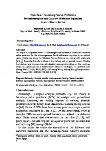
We keep all grid data—the current solution, residuals, source terms, etc.—in fast on-card video memory, storing the data for each progressively coarser grid as a series of images. This allows us to use the fragment pipeline, optimized to perform image processing and texture mapping operations on billions of fragments per second, for our computations. We also eliminate the need to transfer large amounts of data from main memory to and from the graphics card (a common performance bottleneck). To keep the computation entirely on the card, we implement all operations—smoothing, residual calculation, restriction, and interpolation—using fragment shaders that read from a set of input images (textures) and write to an output image. 4.1. Mapping the multigrid algorithm to hardware The multigrid algorithm recursively solves a boundary value problem at several grid resolutions. In our implementation all computationally intensive steps—successive kernel applications, implemented as fragment shaders—are handled by the GPU. Results from one kernel become the input to the next kernel (Figure 1). In other words, we have implemented the multigrid algorithm as a series of stream computations performed in the fragment pipeline, using the CPU to keep track of the recursion depth and rendering state.
Closer in spirit to our work are approaches to GPUaccelerated physical simulation. For example, several NVIDIA demos perform simple physical simulations modeling cloth, water, and particle system physics using vertex and fragment shaders16 . Building on these ideas, Harris et al.8 employ graphics hardware for visual simulation using an extension of cellular automata known as coupled-map lattice. They simulate several fluid processes such as convection, diffusion, and boiling. Rumpf and Strzodka21 explore PDEs for image processing operations such as nonlinear diffusion and express solutions using Jacobi iteration and conjugategradient iteration as rendering passes.
Following this stream processing abstraction, the purpose of each multigrid shader is to operate on data from multi-
smooth
Front
Increasing Time
3.1. Recent related work Two recent publications are particularly relevant. Krüger and Westermann discuss implementation of linear algebraic operators on the GPU11 , while Bolz et al. describe a multigrid solver on graphics hardware, which they demonstrate on visual simulation of fluid flow1 . Although their system is fundamentally similar to ours, the systems also differ in several interesting ways. These differences emerge primarily from the choice of driving problem and the strategies followed for optimization. For example, we target a complex domainspecific engineering code that requires efficient support for periodic boundaries and a way to transform the domain by varying the operator across grid cells (see Section 5.3). As another example, Bolz et al. use a quadrant-stacked data layout to maximize utilization of the four-register GPU vector processors, and report that the bottleneck in the remaining system is the cost of context-switching between OpenGL pbuffers. Our primary goal during optimization has been to eliminate this cost; our data layout makes less optimal use of the GPU memory bandwidth but eliminates contextswitching (see Section 6). c The Eurographics Association 2003.
smooth
Back
residual
Grid i (fine) Front
Back
+ smooth smooth
restrict
Front
smooth smooth
Back
interpolate
Back
Grid i+1 (coarse) Layout in memory
Figure 1: A conceptual illustration of two grids in the multigrid algorithm, each using the front and back surfaces of the solution buffer as alternating source and target. At grid Gi , the smoothing pass is performed by rendering between the surfaces labeled front and back. We then restrict the residual to the front buffer for grid Gi+1 and perform the same smoothing operations on this lower-resolution grid. The approximate solution at Gi+1 is then interpolated back to the higher resolution grid Gi , and the smoothing continues. By using two buffers at each grid level, we can bind one buffer as input and use the other as a rendering target. All arrows between buffers represent render passes.
104
Goodnight, Woolley, Lewin, Luebke, Humphreys / A Multigrid Solver for Boundary Value Problems Using Programmable Graphics Hardware
operator map contains the discretized operator, described in the next section. The red-black map is an optimization used to accelerate fragment odd-even tests for the smooth and interpolate kernels and is described in Section 6. For convenience, these are stored on the front and back surfaces of a second four-channel pixel buffers, letting all buffers share a single OpenGL rendering context.
ple input streams to produce a single output stream. For example, in the smoothing kernel we discretize and store the operator L from Equation 1 as a five-point stencil at every grid cell (storing a separate stencil at every cell enables non-Cartesian grids, such as cylindrical coordinates). Thus the smoothing kernel combines two data streams: one containing the discretized operator Lh and the other containing the current solution Uh . We use texture-mapped polygons to generate these streams as fragments streaming through the GPU fragment engine. Using the OpenGL API, the general procedure for each kernel is as follows:
4.1.2. Smoothing In the multigrid algorithm, smoothing refers to the process of iteratively refining the solution to the boundary value equation 1 at each grid level. The actual implementation will depend on the operator represented by L; in the case of the Poisson equation, L is the Laplacian operator ∇2 . The smoothing kernel applies this operator to a given grid cell, reading from the cell’s immediate neighborhood to compute a new value for that cell. The inputs are simply the current solution U and a five-point discrete approximation of the Laplacian:
• Bind as texture maps the buffers that contain the necessary data. These textures form the input for the kernel. • Set the target buffer for rendering. This buffer forms the output of the kernel. • Activate a fragment shader, programming the fragment pipeline to perform the kernel computation on every fragment. • Render a single quadrilateral with multi-texturing enabled, sized to cover as many pixels as the resolution of the current grid.
∇2Ui j ≈ Ui−1, j +Ui+1, j +Ui, j−1 +Ui, j+1 − 4Ui, j
(2)
where i and j are row and column indices into the grid. The smooth shader applies the operator to each fragment (i.e., grid cell) being rasterized. It also factors in the nonhomogeneous term f , which for heat transfer problems is a spatially varying function of external heat source. Finally, we apply the necessary boundary conditions, as discussed later in Section 4.2. After performing these operations on every fragment, the output represents a closer approximation to the steady-state solution.
Using this procedure, we are able to perform all steps of the multigrid algorithm by simply binding the fragment program, the rendering target, and the appropriate combination of textures as input to the fragment pipeline. Next we describe the principal buffers and the four key multigrid kernels in detail, using as an example our heat-transfer problem modeled by the Poisson equation. 4.1.1. Input buffers The main buffers in the system are the solution buffer, the operator map, and the red-black map. Together these three buffers form the input textures for all of the multigrid kernel shaders. The operator and red-black maps are read-only textures, but the solution buffer also serves as the rendering target for all shaders. As discussed in Section 6, using a single buffer for both input and output avoids context switches, which is crucial for performance with current NVIDIA drivers.
In Jacobi iteration the operator is applied to every grid cell of the source surface, with the output being rendered to the target surface. However, we apply the smoothing using red-black iteration2 , a common method that often converges faster in practice. In red-black iteration the operator is applied to only half of the grid cells at a time, so that one complete smooth operation actually requires two passes.
The solution buffer is a four-channel floating-point OpenGL pixel buffer (a pbuffer) containing two surfaces, exactly akin to the front and back surfaces used for doublebuffered rendering. Each kernel shader reads from one surface of the solution buffer (the source surface) and writes to another (the target surface). After each kernel is run on a given grid level, the source and target surfaces for that level are toggled for the next rendering pass. Each pixel in the solution buffer represents a grid cell, with three floating-point channels containing the current solution, the current residual, and the source term for that cell. We use a fourth channel for debugging purposes.
At each grid cell, the residual value is calculated by applying the operator L to the current solution. For the Poisson equation (where L = ∇2 ), we compute residuals using a single rendering pass of the residual shader and store the result in the target surface in preparation for the restriction pass. The other data from the source surface (current solution and source term) is copied unmodified to the target surface.
4.1.3. Calculating the residual
We can exploit the occlusion query feature of recent graphics chips to determine when steady-state has been reached using the residual calculation. The occlusion query tests whether any fragments from a given rendering operation were written to the frame buffer15 . Every nth iteration— for some user-defined n—we activate a fragment shader that compares the residual at each grid cell to some threshold
The operator and red-black maps are also four-channel floating-point textures in our current implementation. The
105
c The Eurographics Association 2003.
Goodnight, Woolley, Lewin, Luebke, Humphreys / A Multigrid Solver for Boundary Value Problems Using Programmable Graphics Hardware
value ε and kills the fragment (terminating the corresponding SIMD fragment processor’s execution) if the absolute residual is less than ε. If an occlusion query for this operation returns true, we have found the solution to Equation 1 within the tolerance ε. By varying ε we can govern the accuracy, and thus the running time, of the simulation.
real-world situations. We treat boundary values as a simple extension to the state-space of the simulation, enabling the fragment processor to perform the same computation on every fragment and thereby avoiding the need to include boundary-related conditionals in the fragment shader. For example, our multigrid solver allows general boundary conditions, such as Dirichlet (prescribed value), Neumann (prescribed derivative), and mixed (coupled value and derivative). These boundary conditions can be expressed as:
Note that this use of the occlusion query amounts to testing convergence with the L∞ norm: iterate until no cell’s residual exceeds ε. This convergence test is often appropriate for scientific and engineering applications, such as the flapping-wing example in Section 5.3, but may be unnecessarily strict in other cases. For example, visual simulation often uses an L2 norm or even an L1 norm to avoid penalizing local concentrations of error when the overall error across all cells is small. Using these looser convergence tests leads to faster, more consistent run times, at the cost of less predictable error. However, to implement the L2 or L1 norm in a single pass is not possible on current fragment hardware; either the residual must be read out to the CPU (ruinously expensive) or some sort of recursive summation kernel (akin to building a mipmap) must be applied, increasing the cost of the convergence test. One potential architectural solution, helpful in this and other contexts, would be a globally accessible fragment accumulator register—a sort of extended occlusion query that could sum a value across all fragments.
αkUk + βk
(3)
where αk , βk , and γk are constants evaluated at the kth boundary position and Uk is the kth boundary value. The second term on the left hand side is the directional derivative with respect to the normal nk at a given boundary. Equation 3 can be implemented by storing each of the constants in texture memory. For the derivative term we simply replace the fivepoint operator stencil (the discretized operator from Equation 1) with a “boundary condition” stencil. We apply all boundary conditions as part of the smoothing pass; the user can specify a single texture that contains all boundary condition information. Often problems are modeled with periodic boundaries, meaning that cells on one boundary of the domain are considered adjacent to cells on the opposite boundary. For example, allowing periodicity at the vertical and horizontal boundaries of a quadrilateral results in a topologically toroidal domain. Note that periodicity affects the smooth, restrict, and residual kernels, since they all read from a neighborhood of several fragments. A naive implementation of periodic boundary conditions is straightforward: for each fragment being read, simply check within the shader whether that fragment is on a boundary, and if so, use different “neighbor” rules to determine where to sample in the textures when applying the operator. In practice, however, this kind of conditional code should be avoided because the SIMD fragment engine does not natively support branch instructions, so the hardware in fact executes all branches of the code on all fragments, using condition codes to suppress the unwanted results. The naive code is therefore significantly slower than code for the non-periodic boundaries, especially when the kernel must perform some boundaryrelated computation that is wasted on the vast majority of fragments that are not near a boundary.
4.1.4. Restricting the residual If grid Gi represents the ith domain resolution, then Gi+1 is the next-coarser grid level. We restrict the residual from Gi to Gi+1 by setting the rendering output resolution to match the dimensions of grid Gi+1 , then activating a fragment shader that re-samples residual values from Gi using bilinear interpolation and restricts the samples onto the coarser grid (so-called “full weighting”). In other words, the restriction shader takes as input two data streams: a fragment for every grid cell in the Gi+1 domain and a group of fragments in Gi for every cell in Gi+1 . The output becomes the nonhomogeneous term f from equation 1 for the problem to be solved on the coarse grid Gi+1 stored in the appropriate channel of the target surface. As before, the other channels are passed directly through. 4.1.5. Interpolating the correction Finding the approximate solution at grid Gi+1 provides a correction we can interpolate to grid Gi . In this case we set the output rendering resolution to match the dimensions of Gi ; the active fragment shader bilinearly interpolates solution values from one input stream (Gi+1 ) and adds these to another input stream (Gi ).
To efficiently realize periodic boundary conditions, we support two versions of each multigrid kernel: a general shader that works for any fragment (grid cell) in the domain and a fastpath shader that works only for fragments interior to the domain (i.e., those that do not require boundary conditions). When applying the kernel to a domain we split it into two passes: the fastpath shader is rasterized using a rectangle covering the interior fragments of the destination grid, and then the general shader is rasterized as a series of
4.2. Boundary Conditions The ability to specify arbitrarily complex boundary conditions is fundamental to solving boundary-value problems for c The Eurographics Association 2003.
∂Uk = γk ∂nk
106
Goodnight, Woolley, Lewin, Luebke, Humphreys / A Multigrid Solver for Boundary Value Problems Using Programmable Graphics Hardware
cedural shader. We then pick the number of grids and the recursion depth and run iterations of the multigrid algorithm until we determine, using the occlusion query feature, that the system has converged.
Seconds per V-Cycle
2
1
Slow
We used this straightforward application as a testbed, checking the validity and performance of our solver against a custom CPU implementation of the same algorithm developed to support the fluid flow application in Section 5.3. In our tests, the GPU solver agreed with the CPU solver to within floating-point precision.
Fast Path
Fast
0 65x65
129x129
257x257
513x513
1025x1025
Grid Size
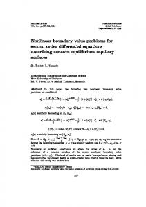
Figure 2: Effects of fastpath optimization. The fully general shader (“Slow”) includes code supporting supporting periodic boundaries, unneeded on most grid cells. The “Fast” shader does not support periodic boundaries. The “Fastpath” optimization uses a two-pass approach to increase speed while supporting periodic boundaries. The slower shader is only used on fragments rasterized on the boundaries, while the interior region of the domain is rasterized using the faster shader.
5.2. Tone mapping for high dynamic range images Images spanning a large range of intensity values are becoming increasingly common and important in computer graphics. These high dynamic range (HDR) images typically arise either from special photography techniques4 or physically based lighting simulations; they are challenging to display due to the relatively low dynamic range of output devices. Several tone-mapping algorithms have been developed to compress the dynamic range of an HDR image. We have used our multigrid solver to implement the Gradient Domain Compression algorithm of Fattal et al.5 This technique applies a non-uniform scaling Φ(x, y) to the gradient of a log-luminance image H(x, y). Specifically, they compute G(x, y) = ∇H(x, y)Φ(x, y). Because Φ is designed to attenuate large gradients more than small gradients, the function G has similar detail to H in areas without large discontinuities, which is exactly the sort of detail-preserving compression desired.
(possibly thick) lines along the boundary fragments of the grid. Since the number of interior fragments is quadratically greater than the number of perimeter fragments, the savings from applying the less expensive fastpath shader on these fragments more than compensates for the cost of binding two shaders and transforming multiple primitives. Figure 2 summarizes the savings achieved by using a fastpath shader. Note that the concept of a fastpath shader was also presented by James and Harris10 and is analogous to splitting the computation in CPU implementations to avoid branch instructions in the inner loop.
Unfortunately, turning G(x, y) back into an image is nontrivial, since G is not necessarily integrable. Instead, they solve the Poisson equation ∇2 I = divG to find the image I whose gradient is closest to G in the least-squares sense. Fattal also uses a multigrid solver to solve this differential equation, although they use Gauss-Seidel iteration while our solver uses red-black iteration.
To simplify the maintenance of periodic boundaries and the construction of the kernels, we employ the common trick of replicating the cells on the periodic boundaries. For example, if a grid has a periodic vertical boundary, the first and last columns of the grid will contain the same data and actually represent the same region of the domain.
5.3. Fluid flow around a flapping wing Fluid mechanics simulations have proven popular choices for acceleration using the GPU; for example, both Harris10, 6 and Bolz1 demonstrate “stable fluids” solvers based on the method of Stam22 . Such solvers are particularly popular in computer graphics because they produce robust and visually convincing (if not entirely physically accurate) fluid flow. Our work on GPU fluid simulation grew out of a desire to accelerate an engineering code that simulates flow around a flapping airfoil using a model by Lewin and Haj-Hariri13 . This code was the motivating problem for our work and remains the most complex model we have used our solver to accelerate.
5. Applications We have applied our system to problems in heat transfer, fluid mechanics, and high dynamic range tone mapping. Here we briefly describe the three applications and their use of the multigrid solver. 5.1. Heat transfer Steady-state temperature distribution across a uniform surface discretized on a Cartesian grid can be solved directly by the multigrid Poisson solver we have presented. We load the initial heat sources into the solution buffer’s finest grid and encode the boundary conditions (such as Dirichlet, Neumann, or periodic) in the operator map, using a simple pro-
The model uses the vorticity-stream function formulation to solve for the vorticity field of a two-dimensional airfoil
107
c The Eurographics Association 2003.
Goodnight, Woolley, Lewin, Luebke, Humphreys / A Multigrid Solver for Boundary Value Problems Using Programmable Graphics Hardware
due to the Joukowski transformation can be accomplished by transforming the discrete approximation to the Laplacian (Equation 2), which requires storing and applying a spatially varying stencil for each grid cell in the smoothing and residual shaders. Rather than hard-coding the coordinate transformations, we use a user-specified shader to compute the operator for the Joukowski transformation at each cell at the beginning of the simulation. This approach allows for very general user-specified domain transformations.
Seconds per V-Cycle
3
2 GPU
CPU
1
0 65x65
129x129
257x257
513x513
1025x1025
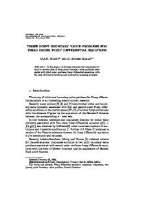
Figure 3 compares performance of the GPU and CPU multigrid solvers on a variety of grid sizes with the parameters used in the flapping wing simulation. The results are summarized in Figure 3, but note that not too much stress should be placed on these results, since the CPU implementation—while far from naive–was not optimized with the same care as the GPU implementation.
Grid Size
Figure 3: CPU vs. GPU comparison. “Seconds per VCycle” is the time to run through a single V-Cycle iteration of the multigrid solver on the fluid mechanics problem. Each V-Cycle used the maximum number of grid levels and performed 8 smooths at each grid level. On large grids, GPU performance begins to significantly exceed CPU performance. These results were obtained using a NVIDIA GeForceFX 5800 Ultra and an AMD Athlon XP 1800 with 512MB RAM.
6. Optimizing the Solver Our initial implementation of the solver operated correctly but was disappointingly slow. We accordingly undertook a series of optimizations targeting some of the obvious performance bottlenecks. We describe this process here as an interesting case study on the issues involved in optimizing general-purpose computation for the GPU.
undergoing arbitrary heaving (vertical), lagging (horizontal), and pitching motions. In the non-inertial reference frame of the airfoil, the vorticity transport equation is modified for the motion of the airfoil and becomes: ∂ζ ∂ζ 1 ∂ζ = −u − v + ∇2 ζ − 2θ¨ (4) ∂t ∂x ∂y Re
A number of potential bottlenecks can limit the performance of a system built chiefly on the fragment processor. We focused first on perhaps the most obvious: the number of instructions in the various shaders and the number of registers used by those instructions. By pre-computing values such as texture coordinate offsets in vertex shaders and by vectorizing the remaining computations where possible (given our data layout, see below), we were able to reduce the instruction count of the four primary shaders by a factor of 3-4 while roughly halving the registers used (Table 1). Note that this includes the “fastpath” optimization described in Section 4.2, which avoids the extra work associated with boundary cells.
∂v − ∂u where ζ ≡ ∂x ∂y is the vorticity, Re is the Reynolds number, and θ¨ is the rotational acceleration of the airfoil. Because the flow is considered incompressible, the velocity components in Equation 4 are found from the stream function ψ:
u=
∂ψ ∂ψ ,v = − ∂y ∂x
(5)
where the stream function is related to the vorticity by ∇2 ψ = −ζ
(6)
At each time step, equations 4 and 6 are solved for the new values of unknowns ζ and ψ, after which equation 5 is solved to obtain the new velocity field. The process is repeated for a predetermined number of time steps.
shader smooth residual restrict interpolate
Bolz et al.1 focus on the Poisson problem for the pressure term; similarly, we focus on the Poisson problem for the stream function in Equation 6. This equation accounts for the bulk of the computation and dovetails nicely with the multigrid Poisson solver presented above. To meet the needs of our fluid model requires extending that solver to handle transformed coordinates. The rectilinear domain is first wrapped into a circular disc and then warped into an airfoil using a Joukowski transformation. These extensions impact the basic solver in two important ways. First, since the cylindrical domain wraps onto itself, two sides of the grid must form a periodic boundary. Second, the distortion c The Eurographics Association 2003.
original fp
fastpath fp
fastpath vp
79-6-1 45-7-0 66-6-1 93-6-1
20-4-1 16-4-0 21-3-0 25-3-0
12-2 11-1 11-1 13-2
Table 1: Instruction and register counts for original and fastpath shaders. For each shader, we give the fragment program complexity (instructions–float registers–half registers) of the original (original fp) and fastpath (fastpath fp) shaders. For the optimized fastpath shaders, we precompute some values such as texture offsets in a vertex program. fastpath vp reports the vertex program complexity (instructions– temp registers).
108
Seconds To Steady State
Goodnight, Woolley, Lewin, Luebke, Humphreys / A Multigrid Solver for Boundary Value Problems Using Programmable Graphics Hardware
10
Very naive
Optimized shaders
Two buffers
One buffer
gle pbuffer, which currently has an absolutely size limit of 2048×2048. Eliminating the final rendering context switch with this arrangement accelerated the final system by an additional 8-10%. Figure 4 shows the relative performance of our various implementations.
5
A simple state machine tracks which surface provides the source and target for each grid level as different kernels are applied. One subtlety arises: following this approach directly can lead to a technically illegal sequence of rendering calls. Alternating buffers across a series of restrict, smooth, and interpolate kernels may result in writing (rendering to) and reading (binding as an active texture) the same surface in the same or successive render passes. Render-to-texture disallows reading and writing from the same surface and requires a glFinish() call between such successive passes15 , but this call proved too heavyweight, ruining performance. One solution is to insert a “copy” kernel which simply renders a grid from one surface to another when necessary to avoid this situation, but this incurs extra cost. In practice, we found that the rules can be broken and a surface used for simultaneous input and output if care is taken to ensure that all fragments output from one pass are written before they are read as input to another pass. By binding new shaders with new rendering state (called uniform parameters in Cg), we
0 129x129
257x257
513x513
1025x1025
Grid Size
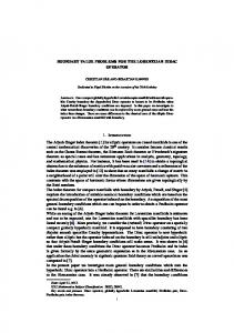
Figure 4: The effect of context switches on performance. Our initial shaders (“Very naive”) were carefully optimized to reduce instruction count and better utilize the vectorized fragment processor (“Optimized shaders”), but all grid levels were stored as separate buffers, so performance was entirely limited by OpenGL context switches. Compacting the grid levels into two pbuffers by stacking grid levels and using front and back surfaces (“Two buffers”) greatly increased performance; further compacting all grid levels into one two-surface pbuffer (“One buffer”) brought a slight additional improvement. Note that at a resolution of 1025×1025, the “Two buffers” implementation ran out of memory, though the others did not.
Surprisingly, the heavily optimized shaders made almost no difference in performance. We had encountered the same bottleneck reported by Bolz et al.1 , namely, the overhead associated with context switches among multiple OpenGL pbuffers on the NV30 platform. Our initial implementation used two separate pbuffers for each grid level; the smooth and residual shaders (which operate on a single grid level at a time) alternated rendering between source and target pbuffers of the same size, while the restrict and interpolate shaders (which move from one grid level to another) would render between pbuffers of different size. The resulting system switched rendering context with every application of every kernel—a naive approach that greatly limited performance. We therefore rearranged the layout of our grids to use only two pbuffers in total. One pbuffer contained two surfaces representing source and target grids for level 0, while the other contained all remaining grid levels–both source and target–in a single surface (see Figure 5). The resulting system eliminated most pbuffer overhead, speeding up the system by a factor of about 3×. However, restrict and interpolate operations entering or leaving grid level 0 still incurred a switch of rendering context. Our final arrangement eliminates this remaining context switch, creating a single pbuffer with each grid level duplicated on front and back surfaces (Figure 5). The layout of grids within a surface is arbitrary; our only requirement was to ensure that we could still fit our largest-sized problem (1025×1025) into a sin-
Figure 5: This figure illustrates the memory layout of our grids in the “Two buffers” implementation (top) and “One buffer” implementation (bottom). Note that in the “Two buffers” case we render back and forth among three surfaces: the front and back surfaces of one pbuffer and a single surface of a second buffer. In the “One buffer” case, we packed all of the grids into two surfaces of a single pbuffer to eliminate context switches.
109
c The Eurographics Association 2003.
Goodnight, Woolley, Lewin, Luebke, Humphreys / A Multigrid Solver for Boundary Value Problems Using Programmable Graphics Hardware
ensure that the pipeline gets flushed between each rendering pass. Alternatively, we could have inserted “no-op” instructions into the fragment pipeline by rasterizing dummy fragments whose results are discarded, but this is a dangerously architecture-dependent strategy.
useful application of stream computing using graphics hardware. We increase performance by keeping all data—current solution, residuals, source terms, operators, and boundary information—on the graphics card stored as textures, and by performing calculations entirely in the fragment pipeline, using fragment shaders to implement the multigrid kernels: smoothing, residual, restriction, and interpolation. In general, one could use our framework to solve a variety of boundary value problems; as a concrete example, we solve the Poisson equation in the context of heat transfer, fluid mechanics, and tone mapping applications. Our solver outperforms a comparable CPU implementation and explores the computational power that can be harnessed by efficient use of graphics hardware.
After adjusting the grid layout to minimize rendering context switches, we implemented several other optimizations. For example, the smooth kernel requires the red-black status of each fragment. Rather than continuously computing this status for each fragment, we store a red-black mask as a texture map for about a 30% speedup. We also verified the occlusion query optimization described in Section 4.1.3, which indeed provides substantial speedup (around 5× on large grids) over testing for convergence on the CPU. Figures 6 and 7 illustrate these savings.
7.1. Analysis of memory bandwidth
Bolz et al. describe a major optimization which we did not employ: domain decomposition for maximum utilization of the vectorized fragment hardware. They “stack” the four quadrants of the grid so that each fragment read or written represents four grid cells. Instead we held to the early design choice to use the simpler mapping described in Section 4.1.1, which stores the current solution, residual, and source term for a single grid cell at each fragment. This was largely to simplify implementation and testing of the complicated boundary conditions we wanted to provide. The optimizations we describe appear to be complementary to the domain decomposition used by Bolz et al., and although we have not done so, it should be possible to apply their approach to our system for significant further speedup.
Analysis of our final system has shown it to be limited by memory bandwidth. For example, on the NV30 we can switch the entire system to use 16-bit half-precision floatingpoint. The resulting system, while not useful for solving realworld problems, runs almost exactly twice as fast as the 32bit full-precision system—a clear indication that memory bandwidth could be the limiting factor. To verify this, we ran additional experiments such as timing many smooth kernels at a single grid level, then comparing the same number of passes with a memory-bound trivial shader that simply outputs a constant value. A comparison of the total bytes accessed per second in each showed that they performed comparably, each accessing approximately 8 GB/sec. Given the nature of the multigrid algorithm, the fact that it is memory-bound is unsurprising. Whether implemented on the CPU or the GPU, the actual computation is relatively minor; when carefully optimized, each kernel performs only a few adds and multiplies at each grid cell. The many memory accesses understandably dominate.
7. Discussion
4
Seconds To Steady State
Seconds To Steady State
We have implemented a general multigrid solver on the NV30 architecture, demonstrating a specific and broadly
Red-black mask
3
Compute red-black
2
1
0 129x129
257x257
513x513
10
NV_OCCLUSION_QUERY glReadPixels()
5
0
1025x1025
Grid Size
129x129
257x257
513x513
1025x1025
Grid Size
Figure 6: Effectiveness of the red-black map. Despite the fact that our solver is limited by memory bandwidth, using the stored red-black map to quickly determine odd-even status for the smooth and interpolate kernels (“One buffer”) remains more efficient than explicitly computing this information in the fragment shader (“Compute red-black”). c The Eurographics Association 2003.
15
Figure 7: Using the occlusion query to test for convergence. Explicitly calling glReadPixels() and examining the residuals on the CPU proves prohibitively expensive on large grids, but using the occlusion query feature allows us to test for convergence while keeping all data on the GPU.
110
Goodnight, Woolley, Lewin, Luebke, Humphreys / A Multigrid Solver for Boundary Value Problems Using Programmable Graphics Hardware
References
Early versions of our system suffered from large amounts of graphics driver overhead and unnecessary computation in each shader. Our work to date has focused on removing these bottlenecks, removing context switches and carefully tuning each shader. Having done that, our system is now limited by memory bandwidth, as we would intuitively expect. Given that, the most important remaining optimizations will be those that address memory usage. 7.2. Limitations While the advent of 32-bit floating point throughout the modern GPU pipeline is a huge leap forward, many realworld science and engineering simulations require even greater precision. We would like to characterize whether workarounds could be developed for higher precision, using techniques similar to those used for “quad-precision” computation in traditional numeric computing (arbitraryprecision techniques also exist, but these seem poorly suited for efficient GPU implementation). Another limitation is the size of video memory, limited to 256 MB on today’s boards; however, this still represents enough memory to model many problems of interesting size. Currently, driver limitations on the size of the floating-point buffers prevent us from approaching the theoretical capacity of the boards: in practice we have been unable to allocate a floating-point texture larger than 64 MB, somewhat limiting the utility of these techniques. 7.3. Avenues for future work We hope to extend the current multigrid implementation to accelerate a wide range of simulations that require fast and efficient solutions to boundary value problems. Our preliminary work raises the possibility that scientists may soon be able to accelerate their simulation substantially by investing in a commodity graphics card. We are particularly interested in parallelizing the multigrid computation, augmenting existing computational clusters with inexpensive graphics cards to provide speedups on some problems. Finally, we wish to explore general computational frameworks for the use of GPU as a sort of streaming coprocessor for computation-intensive tasks. Acknowledgements We would like to thank David Kirk and Pat Brown, Matt Papkipos, Nick Triantos and the entire driver team at NVIDIA for providing early cards and excellent driver support; James Percy at ATI and Matt Pharr at NVIDIA for demystifying the fragment pipeline; Mark Harris, Aaron Lefohn, and Ian Buck for productive discussions on general-purpose GPU computation; and the anonymous reviewers for their thorough and constructive comments. This work was supported by NSF Award #0092793.
111
1.
Jeff Bolz, Ian Farmer, Eitan Grinspun, and Peter Schröder. Sparse matrix solvers on the GPU: Conjugate gradients and multigrid. ACM Transactions on Graphics, 22(3), July 2003.
2.
W.L. Briggs, V.E. Henson, and S.F. McCormick. A Multigrid Tutorial. Society for Industrial and Applied Mathematics, 2000.
3.
Nathan Carr, Jesse Hall, and John Hart. The Ray Engine. In Proceedings of SIGGRAPH/Eurographics Workshop on Graphics Hardware, September 2002.
4.
Paul Debevec and Jitendra Malik. Recovering high dynamic range radiance maps from photographs. In Proceedings of SIGGRAPH 1997, pages 369–378, August 1997.
5.
Raanan Fattal, Dani Lischinski, and Michael Werman. Gradient domain high dynamic range compression. ACM Transactions on Graphics, 21(3):249–256, July 2002.
6.
Mark Harris. Flo: A real-time fluid flow simulator written in Cg, 2003. http: //www.cs.unc.edu/~harrism/gdc2003.
7.
Mark Harris. GPGPU: General-purpose computation using graphics hardware, 2003. http://www.cs.unc.edu/~harrism/gpgpu.
8.
Mark J. Harris, Greg Coombe, Thorsten Scheuermann, and Anselmo Lastra. Physically-based visual simulation on graphics hardware. In Proceedings of SIGGRAPH/Eurographics Workshop on Graphics Hardware, pages 109–118, August 2002.
9.
Kenneth E. Hoff III, John Keyser, Ming C. Lin, Dinesh Manocha, and Tim Culver. Fast computation of generalized Voronoi diagrams using graphics hardware. In Proceedings of SIGGRAPH 1999, pages 277–286, August 1999.
10.
Greg James and Mark Harris. Simulation and animation using hardwareaccelerated procedural textures. In Proceedings of the 2003 Game Developers Conference. CMP Media, March 2003.
11.
Jens Krüger and Rüdiger Westermann. Linear algebra operators for GPU implementation of numerical algorithms. ACM Transactions on Graphics, 22(3), July 2003.
12.
E. Scott Larsen and David K. McAllister. Fast matrix multiplies using graphics hardware. In Proceedings of IEEE Supercomputing 2001, November 2001.
13.
Gregory C. Lewin and Hossein Haj-Hariri. Modeling thrust generation of a twodimensional heaving airfoil in a viscous flow. Journal of Fluid Mechanics, 2000.
14.
William R. Mark, Steve Glanville, and Kurt Akeley. Cg: A system for programming graphics hardware in a C-like language. ACM Transactions on Graphics, August 2003.
15.
NVIDIA. OpenGL Extension Specifications, 2002. http://developer. nvidia.com/view.asp?IO=nvidia_opengl_specs.
16.
NVIDIA. GeForceFX, 2003. PAGE=fx_desktop.
17.
Mark Peercy, Marc Olano, John Airey, and Jeffrey Ungar. Interactive multi-pass programmable shading. In Proceedings of SIGGRAPH 2000, pages 425–432, August 2000.
18.
William H. Press, Saul A. Teukolsky, William T. Vetterling, and Brian P. Flannery. Numerical Recipes in C: The Art of Scientific Computing. Cambridge University Press, second edition, 1992.
19.
Kekoa Proudfoot, William Mark, Svetoslav Tzvetkov, and Pat Hanrahan. A real time procedural shading system for programmable graphics hardware. In Proceedings of SIGGRAPH 2001, pages 159–170, August 2001.
20.
Tim Purcell, Ian Buck, William Mark, and Pat Hanrahan. Ray tracing on programmable graphics hardware. ACM Transactions on Graphics, 21(3):703–712, July 2002.
21.
Martin Rumpf and Robert Strzodka. Nonlinear diffusion in graphics hardware. In Proceedings of Eurographics/IEEE TCVG Symposium on Visualization, pages 75–84, May 2001.
22.
Jos Stam. Stable fluids. In Proceedings of SIGGRAPH 1999, pages 121–128, August 1999.
23.
Chris J. Thompson, Sahngyun Hahn, and Mark Oskin. Using modern graphics architectures for general-purpose computing: A framework and analysis. In Proceedings of IEEE/ACM International Symposium on Microarchitecture, pages 306–317, November 2002.
http://www.nvidia.com/view.asp?
c The Eurographics Association 2003.
Goodnight, Woolley, Lewin, Luebke, Humphreys / A Multigrid Solver for Boundary Value Problems Using Programmable Graphics Hardware
1
0.5
0
-0.5
-1
X
Colorplate 1: Flow around a flapping wing. We accelerate a vorticity-stream function fluid mechanics model using our multigrid solver for the Poisson problem in the stream function solution.
Colorplate 2: A high dynamic range image compressed with our gradient-domain tone mapping application. The top row shows some constituent images used to produce the HDR image; the bottom row shows compressions using multigrid CPU (left) and GPU (right) Poisson solvers.
c The Eurographics Association 2003.
135