Motion Planning for a Modular Self-Reconfiguring Robotic System CEM ÜNSAL*, HAN KILIÇÇÖTE, MARK E. PATTON, and PRADEEP K. KHOSLA Institute for Complex Engineered Systems, Carnegie Mellon University, Pittsburgh, PA, 15213-3890, USA (*
[email protected])
Abstract. In this paper, we address the issue of motion planning for a bipartite class of modular self-reconfiguring robotic system (I-Cubes) that is a collection of active elements providing reconfiguration (3-DOF manipulators called links) and passive elements acting as connectors (cubes). The links, capable of attaching/detaching themselves from/to cubes, can position and orient the cubes. Current solutions for motion planning and reconfiguration of I-Cubes include multilayered planners that divide a given problem into tractable sub-problems to be evaluated using heuristic methods. The system implementation, its representation in simulation, search algorithms resulting from this representation, and simulation examples are presented. Keywords: self-reconfiguration, metamorphic robots, path planning 1. Introduction Statically stable gaits for mobile robots include wheels, threads, and similar mechanisms. These methods, although providing fast locomotion on level ground, generally do not provide capabilities such as climbing stairs, or moving over obstacles. A robot that can move with relative ease on flat terrain and an ability to climb over large obstacles is yet to be designed. Recent progress in component and sensing technologies move research thrusts on small mobile robots toward smaller scales, and multi-sensor/multi-actuation capabilities further. Applications for groups of small mobile robots working in unstructured environments are slowly emerging. A sufficient number of robotic modules combined as a single entity would be capable of self-reconfiguring themselves into defined shapes. A large group that can change its shape according to the locomotion, manipulation or sensing task at hand will then be capable of transforming into a snake-like robot to travel inside a air duct or tunnel, a legged robot to move on unstructured terrain, a climbing robot that can climb walls or move over large obstacles, a flexible manipulator for space applications, or an extending structure to form a bridge. Designing a modular system with identical elements has several advantages over large robotic systems. The homogeneity can provide faster production at a lower cost. A modular selfreconfiguring system would be capable of removing malfunctioning elements from the group and reconfigure its elements. Previous research on modular robotic systems includes manipulators that can be designed according to task specification [1,2], and cellular systems as self-
1
organizing manipulators [3]. These and similar ideas on modularity have been extended to modular structures that can self-reconfigure. Existing 2-D selfreconfiguring systems include Inchworm [4], and self-organizing robots [5] moving in vertical planes, Fractum [6], and metamorphing hexagonal modules [7] moving in horizontal plane. Recent 3-D systems are Polypod and Polybot that combine different gaits [8, 9], robotic molecule [10] and self-reconfigurable structure [11] that are both capable of changing shape using neighboring elements as pivot points. In the following sections, we discuss the 3-D reconfiguration for a bipartite class of modular self-reconfiguring robotic system. Our aim is to combine different gaits and task-oriented modules with self-reconfiguration capabilities. 2. I-Cubes: A 3-D Modular Self-Reconfigurable System For self-reconfiguration, a modular system must have several essential properties, such as geometric, physical, and mechanical compatibility among individual modules. Furthermore, several design issues need to be considered for the system to be autonomous. I-Cubes are a bipartite modular system, i.e., a collection of independently controlled mechatronic manipulators (links) and passive connection elements (cubes). Links are capable of connecting to and disconnecting from the faces of the cubes; they can therefore move from one cube to another, or move a cube (Figures 1 & 2). We envision that all links and cubes are capable of permitting power and information flow to attached modules. The system has the following properties: •Modules can be independently controlled. •All modules have the same characteristics, and are compatible. •The 3-D structure fits a cubic lattice to guarantee interlocking of neighboring
modules, i.e., distance between cubes in idle position is constant. •Links have sufficient degrees of freedom to complete motions in 3-D.
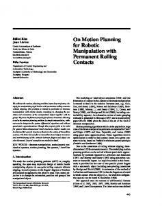
Since the actuation for self-reconfiguration is provided by the links, cubes can be used to provide computation, sensing and power resources. If the modules are designed to exchange power and information, the cubes may be equipped with batteries, microprocessors and sensors to be the decision-making elements while the links become the ‘muscles’ of the system. It is also possible to remove some of the attachment points on the cubes to replace them with wheeled or threaded systems for faster locomotion. Specifically, we envision small robots that can reposition themselves to form a group that is capable of self-reconfiguring in order to move over obstacles that a single robot cannot overtake. Similar scenarios that combine different gaits with shape reconfiguration include stair climbing and traversing pipes. As seen in Figure 1, the size definitions for the links and the cubes are dependent. If the length of a cube edge is L, then the links should have four sections with indicated lengths. The three rotational degrees of freedom for the links are provided by the joint J2 at the middle, and the joints located at end segments (J1 and J3). J1 and J3 are both capable of providing continuous 360-degree rotations, while J2 can only rotate 270 degrees. The design parameters given above and the attachment capabilities enable links to (a) move from one cube face to another, (b) move one cube while attached to another, and (c) move from one cube to another (Figure 2). A
2
cube consists of six faceplates with attachment points for link connectors. Cubes do not contribute to the self-reconfiguring motions with the exception of the motion to lock the link connector in place. A cube attached to a link can be (i) rotated, (ii) translated in vertical or horizontal plane, or (iii) act as a pivot point for a moving link. The role of the cube depends on the position and motion of the active link as well as the connections formed by all modules.
J2 J1
J3
L
L/2
L
detach
attach 2 1
rotate
4
A
3
B
rotate
rotate 1
(a)
(b)
L 2 attach 1 rotate
Fig. 1. Geometric constraints and joint definitions for the links
detach
3
4 rotate
(c) Fig. 2. Examples of link motions
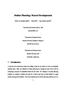
3. Implementation and Experiments For the prototypes shown below, the module bodies are created using a fused deposition modeling (FDM) machine. The link and cube bodies, generated in ProEngineer©, are assembled with off the shelf components. A link equipped with all mechanical and electrical components weights approximately 370gr. The length L is 8cm. A cross-shaped attachment mechanism designed to connect the links and the cubes is actuated using an SMA wire (Nitinol) and spring mechanism. One faceplate for a cube weights approximately 20 gr. The depth of a faceplate is 1cm. Therefore, a volume of 6×6×6 cm3 is available for computational, sensing elements and power source. The actuators on the links and the cubes are controlled by microprocessors connected to a graphic user interface (GUI). Two 6V 650mAh rechargeable batteries are used to power all servos on the links, the attachment mechanisms, and the microprocessors. The details of the mechatronic design are given in [12]. The prototypes are used to test the feasibility of the system. Tests show that a link can transfer from a horizontal plane to vertical plane, and vice versa, using three available degrees of freedom. Similarly, a link can move from one cube face to another as well as from one cube to another (Figure 3a-b) The links are also capable of moving and exchanging cubes. As seen in Figure 3c-d, one link (left) moves the cube into position and orients it for another link to attach to and move the cube to its next destination.
(a) (b) (c) (d) Fig. 3. (a-b) A link transferring from one cube to another; (c-d) two links exchanging a cube.
3
4. Three-dimensional Reconfiguration By combining several link actions (attachment/detachment and joint rotations), it is possible to find solutions for a group of cubes and links moving and/or selfreconfiguring from one position/shape to another. Figures 4 and 5 show two groups of four cubes and four links (4C4L). Figure 4 illustrates a scenario where a 4C4L group is moving to higher ground. During reconfiguration, the connections between modules kept such that the group forms a single connected graph at any time. We assume that a link can only carry a cube and another link attached to this cube. This manual solution takes into account the orientation of the cubes, and keeps the same cube faces on the ground. In Figure 5, the group on the ground is moving to the right. The sequence of actions depicted here is one of many possible solutions. Another example that combines a self-reconfiguration and faster locomotion is shown in Figure 6. The leftmost robot in the first image has a camera, but cannot see what is on/behind the obstacle. These wheeled robots can move into position to form a group and self-reconfigure to lift the camera-equipped robot. Required number of faces with attachment points is two for the camera-equipped robot. It is also possible for a larger group to self-reconfigure into a tower to lift a surveillance robot to see beyond relatively larger obstacles [13]. This scenario illustrates an important characteristic of the system. A heterogeneous group of small robots combines individual robot capabilities with self-reconfiguration to complete a task that is not possible for individual robots.
Fig. 4. 4L4C group climbing a stair: manual solution.
(a)
(b) (c) Fig. 5. 4L4C group moving to right
(a)
(b) (c) (d) Fig. 6. Two carrier robots lifting another
(d)
(e)
(e)
4.1 System Representation for Planning In this section, we introduce a grid representation for groups of m cubes and n links. For a given m-cube n-link combination, there are multiple states that the group can take depending on the relative positions and shape of the modules. The number of possible states grows exponentially with the number of cubes and/or links. A group of m cubes and n links can be represented with a three-dimensional cell grid of size d×d×d where d = (2m-1) + 4 (Fig. 7). Each cell may be occupied only by a single cube or link. Each cube can occupy only one cell, while the links occupy two or three
4
cells depending on their shapes (See Fig. 7). We discretize the link positions at 90degree joint angles. 3 x 3 grid (m = 2)
Global origin g
-2 –1
0
1
2
3
4
x
7 x 7 grid (2m+3)
Cube pos. = [0 2 2]
-2 -1 y=2
1 Link pos. A = [0 2 3] C = [1 2 3] B = [0 2 3]
Cube pos. = [2 2 0]
0
2 3
Link pos. A = [2 2 1] C = [1 2 1] B = [1 2 2]
4 z (a) (b) Fig. 7. (a) Grid definition, and (b) 2 of 4 possible shapes: link ‘looking’up or down at the same position
The cells in the 3-D grid are represented by their local coordinates where the origin is defined as the cell closer to a global origin. Global positions of the links and cubes can be evaluated by combining the local coordinate system and the global position of the grid. We define the following based on the link and cell definitions: (i) A state S is a quadruple {C, L, f, d} where C and L are sets of vectors indicating cube positions and link positions and shapes, f is a binary relation between C and L indicating the connections, and d defines the size of the grid. (ii) A node N is a couple {S, g} where S is a state and g is its global position. A given problem with initial and final configurations can be represented as a pair {No, Nf} and have multiple solutions based on the sequence of link actions. For a given state S, there are 24 actions for each link. These actions define a sequence of link detachments and rotations. We assume that all links automatically attach to a cube at the end of an action if there is such a cube. All possible actions aij (i=1,… ,24, j=1,… ,n) are relations from one state to another, and are associated with translations tij indicating possible change in global coordinates of the node N associated with the state S. For example, the action in Figure 2b is “detach others at A, fix B, B +” where all the links except the active link connected to the moving cube are detached, the end B is assumed to be fixed, and the joint at end B is rotated clockwise. These actions aij are actually a group of actuation commands for attachment mechanisms on the cubes, and for servos on the links. For a link to be able to move, the desired location and the path of the link (and the cube that may be attached) must be clear: the cells associated with new location, and path of the link (and cube), and some of the cells next to the initial and final cube positions should not be occupied by links, cubes or obstacles. An action aij acting on a state will create a new state if a link or cube changes position. The associated translation tij may have non-zero elements if there is a cube relocation that changes the definition of the cube closer to the origin. A state transition diagram is a graphical representation of all the states for an nCmL combination with the pairs (aij, tij) defined between states. Figure 8a shows part of the transition diagram for 1L2C case, where each edge indicates one or more actiontranslation pairs. Total number of possible states for a 1L2C group is 36 if the link is
5
not allowed to detach from the cubes. If link can detach from the cubes, the number is 1404. For an attached 2L2C group, total number of states is 4518. x
x a1,11
a1,19
S1
S4
a1,12 z
[0 [0 g = [2 0 2] + [2 [ 2
0 − 2] 0 0] 0 − 2] 0 0]
a1,20 z
g = [2 0 2]
(a) (b) Fig. 8. (a) Transitions from state #1 and (b) action/translation definitions from state #1 to state #4
4.2 Complexity The number of possible states increases exponentially with the number of cubes and links. Note that for a given position of cubes, there may be several states represented by the same connection matrix f, but have different link positions and shapes. Each connection between states on the transition diagram represents one or more actions and their associated state-to-state translation in 3-D. For example, as seen in Figure 8b, there are four possible actions from state #1 to state #4, each associated with a different translation value. While solving a problem for a large group of cubes and link, one has to generate the search graph of nodes Ni evaluating all possible states located at all possible positions. This new graph of nodes is significantly larger that the state transition diagram. Finding a solution with minimal number of actions corresponds to a shortest path problem on this graph of nodes. This problem can be solved using known methods such as A* search where the cost of actions is associated with 90-degree link motions and the cost estimate for reaching the goal can be chosen as the total or average distance of all cubes and/or links to their goal positions. The computation of this search graph is computationally exhaustive due to exponential growth in graph size based on the number of cubes and links. Finding an upper bound on the number of link actions for a given cube motion proves to be difficult. However, following the discussion of [14], we can state that the number of cube motions for any given problem with a single cube relocation cannot be greater than the perimeter, i.e., neighboring cells of the group of cubes. This perimeter for groups of cubes in 3-D is found to be 10n+8. Therefore, the total number of cube motions for a single cube relocation is at most O(n). For each cube move, the total number of links that detach/attach or rotate is m (i.e., the number of links) at maximum. This is assuming all the links need to moved; the actual number is usually much less than m. For each link, the maximum number of ‘jumps’ from one cube to another is limited to n-1. While attached to a single cube, a link can reach any position with a maximum face transition of five (Again, the actual number is less than this). Therefore, a loose upper bound on the number of link motions for a single cube relocation is O(m.n2). The total number of cube motions depends on the initial and final configurations. For the problems solved by the planner, we see that the number of link motions is much less than the possible orders of magnitudes given above for relatively small groups. Note that the discussion here does not consider interleaved link actions, which is the case most of the time.
6
5. Algorithms Finding a sequence of actions for a given problem involving m cubes and n links where m, n > 2, is fairly difficult due to the nature of the problem as indicated above. Evaluating all possible states/nodes for large group of modules is not possible. However, we might be able find solutions by carefully evaluating states/nodes. For example, the states and nodes necessary to solve a problem can be generated only when necessary as indicated in Section 6. It is also possible to divide the problem into sub-problems that can be solved by using heuristics methods. If we are to generate a sequence of actions for a given Problem {No, Nf}, this solution can be divided into subsequences so that the difference between the states corresponding to the beginning and end of each subsequence is a single cube relocation. If there is a solution from No to Nf, then it can be divided into subsequences that are solutions to less complex and ‘local’ problems. Each of these sub-problems can be solved using standard heuristic methods. For a given single cube motion, simple heuristics can find a solution for the necessary link motions using the evaluation functions mentioned above. To generate the sub-problems, i.e., to find the individual cube motions to be considered, we can use the methods described in [13] or take the approach given in Section 5.1. 5.1 Two-Level Planner The planner for cube and link motions attacks the problem in two steps. At the lower level, the sub-problems involving limited cube motions are solved, finding a sequence of link actions leading to the solution. At the higher level, individual cube motions are evaluated based on the goal position and shape. The results presented here are generated by two similar approaches. The first approach (we call SolverIC) evaluates the desired position for each cube based on occupied goal positions and cube distances to unoccupied positions. These positions are sorted and updated based on the feasibility of the required motions (e.g., cubes must clear all obstacles and other cubes, and keep a maximum distance of 4 using Manhattan metric as well as maximum distance of 2 in each direction to the closest neighbor), possible conflicts between two desired positions, and the requirements for a cube to be in a specific position as pivot. After the negotiation phase, the cubes that are permitted move to their new positions and the cycle is repeated. One or more cubes can move at a time; maximum number of cubes allowed to move is a user-defined variable. The second approach (SolverFS) uses a slightly different approach in evaluating the desired cube motions. All possible cube motions are again filtered using the motion requirements, and resulting nodes are sorted using an evaluation function that defines the distance to the goal node. The cube motion that is evaluated to be the best action is carried out if the pivot cube requirements are met. This algorithm identifies a single cube to be moved at a given step. Both algorithms provided very fast solutions for the problems we have tested. The second approach usually returns better solutions for cases similar to one given in Figure 5, because it evaluates resulting nodes with respect to their distance to goal position. However, the first approach (SolverIC) can handle larger groups of cubes evaluating simultaneous cube motions. Figure 9 shows initial and final conditions for a 27-cube problem and the snapshots of a solution for the given problem. Total number of steps is 22. Note that their success rate is based on the number and diversity of the allowed cube motions.
7
(t = 0)
(t = 1) (t = 6) (t = 14) (t = 22) Fig. 9. 27 cubes dissolving: snapshots of a solution with simultaneous cube motions
5.2 Pruning the Search Space The motion planner, while evaluating states (and nodes) resulting from specific actions uses several rules to prune some of these nodes from the search space. Although the new states are added to the transition diagram, if the action is found to be not permissible for the present node (i.e., present state at the given global position), the resulting node is not added to the search list. Possible reasons for a new node to be rejected are: • • • • •
Link/cube motion does not clear obstacles Cube is swept on the ground or slid over obstacles There are constraints on the total number of supported cubes Cubes move beyond the user-defined ranges The overturning moment resulting for link/cube motion causes instability
All of these rules except the last are easy to check. For the stability analysis, the calculations are slightly more complex, and the order of complexity of the algorithms defined below are O(n2). The current stability analysis is limited to overturning, and does not consider sliding stability. The surface on which the robot rests is assumed to be flat, level, and a hard stable surface capable of supporting the robot without deflection or distortion. The analysis does take into account the cubes placed on obstacles at different elevations, but does not account for sloped surfaces. The analysis is independent of the plane of analysis; it can be performed for any type of force, similar to gravity, static in nature, irrespective of its direction. The stability analysis is simplified by the geometry of the robot. All cube faces are either perpendicular or parallel to the faces of adjacent cubes to which they are linked. The link geometry in terms of arm length is fixed, and movements can only result in motions that end in cubes being translated a fixed distance (on a plane perpendicular to one of the default axes) or rotated by 90 degrees at its center. The location of center of gravity on the plane normal to the direction of gravity is compared to the footprint of the robot, which will be stationary during a projected move. If the location of the center of gravity of the entire robot including the moving portion falls within the base of the stationary portion during the course of the movement, the move is found to be safe and will not cause the robot to overturn. If the location of the center of gravity moves to outside the base area, the motion will cause the robot to turn over. The effective base area of the robot is the area of the stationary portion of the robot that is defined by the boundary formed by the outermost points. These points are simply the corners of the cubes that lie on the ground, or obstacles, and are stationary for the particular move for which this analysis is done. The base area calculation involves finding the ‘convex hull’ of the base points that form the outer boundary of the cubes that do not move. As a first step, the base cubes are identified. From the
8
base cubes, a collection of the points forming the convex hull is sorted out. Note that the changes in the convex hull at each time step are due to at most one cube relocation. The results of the algorithm are compared to several cases (such as the one in Figure 10d) evaluated in Working Model 3D. 6. Simulation Results The planners described above are used to generate the solutions given in this section. Figure 5 shows a 4C4L group that moves to the right. The difference between initial and final positions is 4 units. The total number of 90-degree link actions to move the group to its desired position is 22. This solution is generated using a high-level SolverFS. Only the final positions of the cubes are defined. For sub-problems, only the cube positions are considered even if final link positions are given. The planner created four sub-problems to be solved by the low-level solver. The maximum number of states and nodes evaluated for the sub-problems are 453 and 108 respectively. Average Manhattan distance over all cubes is used to evaluate the node distance to goal. The snapshots in Figure 5 belong to this solution. We have also tried to solve this problem using a single A* solver with node-to-node transition cost of 1 and a factor of 2 multiplied with the average cube distance to the goal positions (using Manhattan metric). The total number of actions is again 22, with 2169 nodes and 1542 states generated. Only 581 nodes are evaluated to reach the solution. It is interesting to note that these and the solution given by 3-level solver defined in [13] are found to be the same. Figure 10 shows snapshots of a solution to stair climbing problem of Figure 4 obtained using a high-level SolverFS. Only the final positions of the cubes are defined in the problem. Total number of link motions to reach the goal is 56. Four subproblems (initial states shown in Fig. 10a, b, c, and e) are generated. Most difficult sub-problem is the third. Total number of nodes generated for this section is 8501 of which 3244 are evaluated. There were 7555 states associated with this sub-problem. The snapshots show the beginning node of each sub-problem and the final position. A solution for this problem could not be found using the algorithm described in [13] due to the lack of additional rules for higher level solvers. Similarly, this new approach is capable of finding exact solutions to other problems given in [13] as well as the scenario described in Figure 6. The total number of actions in the computer-generated solution for this case is 10.
(a) (b) (c) (d) (e) (f) Fig. 10. A solution using FS-A* pair: (a) Initial, (f) final, and (b,c,e) beginning nodes for sub-problems
7. Concluding Remarks We have introduced our results of a divide-and-conquer approach to motion planning for a class of modular self-reconfiguring robotic system. Our attempts to find fast solutions take advantage of defining tractable sub-problems for a given pair of initial
9
and final conditions. Separating the problem into smaller, less complex cases has its advantages; however, issues such as backtracking, algorithmic complexity for lowlevel planning are yet to be answered. Note that the algorithms described here are capable of finding solutions for initial and final conditions with no overlapping link or cube positions. In many cases, it is advantageous to combine two or more sub-problems involving single cube motion. In addition, we have found that the high-level planner sometimes returns sub-problems that lead to unnecessary link motions when combined. It is possible to design decision mechanisms to combine sub-problems, reconsider cube motions, or refine the sequence of link motions evaluated by low-level planner. However, the design of these mechanisms is not straightforward. Furthermore, the planner still suffers from the lack of backtracking capabilities for cube motions. We are currently working on incorporating semantic representation of the group into lowlevel search for speeding up the search process. Our plans also include extending our motion planners using other pruning methods and finding alternatives to heuristic search carried out at the lower level. References [1] Chen I.-M., J. W. Burdick. (1993) Enumerating Non-Isomorphic Assembly Configurations of a Modular Reconfigurable Robotic System, IEEE Intl. Conf. on Intel. Rob. & Syst., 1985-92. [2] Paredis, C.J.J., H. B. Brown, and P. K. Khosla. (1997) A Rapidly Deployable Manipulator System. Robotics and Autonomous Systems, 21, 289-304. [3] Fukuda, T., and Y. Kawauchi. (1990) Cellular Robotic System as One of the Realization of Self-Organizing Intelligent Universal Manipulator, IEEE Conf. on Rob. & Auto., 662-667. [4] Kotay, K., and D. Rus. (2000) Inchworm Robot: A Multi-functional System, Autonomous Robots, 8, 53-69. [5] Hosokawa, K., et al. (1998) Mechanisms for self-organizing robots which reconfigure in a vertical plane. Distributed Autonomous Robotic Systems, 3. Springer-Verlag, NY. 111-118. [6] Yoshida, E., et al. (1998) Experiments of Self-Repairing Modular Machine. Dist. Autonomous Robotic Systems 3. Springer-Verlag, NY. 119-128. [7] Pamecha, A., et al. (1996). Design and Implementation of Metamorphic Robots, Proc. ASME Design Engineering Technical Conf. & Computers in Engineering. Conf. [8] Yim, M. (1994). New Locomotion Gaits, Proc. IEEE Intl. Conf. on Rob. & Auto. [9] Yim, M., D. Duff and K. Roufas. (2000) PolyBot: a Modular Reconfigurable Robot, Proc. IEEE Intl. Conf. On Robotics & Automation, 514-520. [10] Kotay, K., et al. (1998) The Self-reconfiguring Molecule: Design and Control Algorithms. Algorithmic Foundations of Robotics. A.K. Peters. [11] Murata, S., et al. (1998) A 3-D Self-Reconfigurable Structure, IEEE Intl. Conf. on Robotics & Automation, 432-439. [12] Ünsal, C., and P. Khosla (2000) Mechatronic Design of a Modular Self-Reconfiguring Robotic System, Proc. IEEE Intl. Conf. on Robotics & Automation, 1742-1747. [13] Ünsal, C., et al. (2000). A Modular Self-reconfigurable Bipartite Robotic System: Implementation and Motion Planning, Tech. Rep., ICES, CMU, Pittsburgh, PA. [14] Chirikjian G.S., and A. Pamecha. (1995) Bounds for Self-reconfiguration of Metamorphic Robots. JHU Technical Report, RMS-9-95-1.
10