Mapping the Spatio-Temporal Evolution of Irrigation in the Coastal Plain of Georgia, USA Marcus D. Williams, Christie M.S. Hawley, Marguerite Madden, and J. Marshall Shepherd
Abstract
This study maps the spatial and temporal evolution of acres irrigated in the Coastal Plain of Georgia over a 38 year period. The goal of this analysis is to create a time-series of irrigated areas in the Coastal Plain of Georgia at a sub-county level. From 1976 through 2013, Landsat images were obtained and sampled at four year intervals to manually detect Center-Pivot irrigation (CPI) systems in the analysis region. During the 38 year analysis period there was a 4,500 percent increase in CPI systems detected that corresponded to an approximate 2,000 percent increase in total acreage. The bulk of the total acreage irrigated is contained in southwest Georgia, as seven counties in the region contained 38 percent of the total acreage irrigated in 2013. There was substantial growth throughout the entire Coastal Plain Region, but southwest Georgia was identified as the most heavily irrigated region of the state.
Introduction
Agriculture has always been critical for sustaining human life on Earth. Improving technology and agricultural practices made it possible for world food production to double over a 31 year period between 1960 and 2000 (Tilman, 1999), which is part of a larger increased agricultural production in the 20th Century known as the Green Revolution (Evenson and Gollin, 2003). In the year 2000, approximately 15 million square kilometers of the global land cover was dominated by cropland (Ramankutty et al., 2008). With the current world population of 7.3 billion, which is expected to reach 11.2 billion by the year 2100 (UN Department of Economics and Social Affairs) and the growing demand for biofuel production (Evans, 2009) the need for agricultural landscapes could potentially increase in the future. One catalyst from the rapid improvement of agricultural production was the large expansion of irrigation (Tillman et al., 2001). Irrigation can be defined as land areas that receive full or partial application of water by artificial means to offset periods of precipitation shortfalls during the growing period (Ozdogan et al., 2010). In 2000, it was estimated that 2.8 million km2 were irrigated, with this number forecasted to increase 5.29 million km2 by 2050 (Tilman, 2001). Irrigation, much like urbanization, acts to alter the natural landscape properties such as partitioning latent and sensible heating at the surface of the Earth which can impact surface temperature and surface moisture transport. Understanding the extent and usage of irrigation is imperative in answering questions about future water resources, as it is estimated that irrigation uses over 70 percent of the world’s consumption of freshwater (Boucher, 2004; Velpuri et al., 2009). Irrigation accounts for Marcus D. Williams and Christie M.S. Hawley are with the USDA Forest Service, Southern Research Station, Center for Forest Disturbance; 320 E. Green Street, Athens, GA 30602 (
[email protected]). Marguerite Madden and J. Marshall Shepherd are with the University of Georgia, Department of Geography, 210 Field St. No. 204, Athens, GA 30602.
PHOTOGRAMMETRIC ENGINEERING & REMOTE SENSING
approximately 60 percent of consumptive use of freshwater in the United States where estimates show that over 222,577 km2 of cropland are irrigated (Braneon, 2014; Minchenkov, 2009). For Georgia, it is estimated that approximately 5.5 billion gallons of water per day were withdrawn from surface and ground waters in 2004 (Barnes and Keyes, 2010). Agricultural water use during 2005 totaled 752 million gallons per day for irrigation, with the highest rate of irrigation occurring in the Coastal Plain region of Georgia. The primary crops irrigated in Georgia are maize, cotton and peanuts as they accounted for approximately 68 percent of the total irrigated acreage in 2002 (Braneon and Georgakakos, 2014). Agricultural water use in Georgia is also tied into the ongoing dispute between Georgia, Florida, and Alabama over water use in the Apalachicola-Chattahoochee-Flint (ACF) River Basins known as the “Tri-State” waters wars. Georgia is the upstream water user and the heavy agricultural water usage in southwest Georgia impacts the amount of fresh water that reaches Apalachicola Bay in Florida which supports a multi-million dollar shellfish industry. Research has shown that irrigated croplands can impact land-atmosphere interactions and fresh water supply. Various modeling and observational studies have demonstrated that irrigation influences climate at the local, regional, and global level by enhancing evapotranspiration, altering precipitation patterns, as well as impacting minimum temperature, maximum temperature, and diurnal temperature range (Barnston and Schickedanz, 1984; Greets, 2002; Adegoke et al., 2003; Boucher, 2004; Kueppers, 2007; Lobell and Bonfils, 2008; DeAngelis et al., 2010; Sen Roy et al., 2011; Cook et al., 2014 Shukla et al., 2014, Williams et al., 2015) These activities present a need for accurate and detailed geospatial information on irrigated croplands (Pervez and Brown, 2010). In the United States, most mapping efforts are focused primarily on the California and the Great Plain regions. To expand and contribute to existing knowledge on the spatial and temporal changes in irrigation in Georgia, this analysis maps center pivot irrigation systems (CPI systems) through visual interpretation of Landsat satellite imagery. This shape-based method of mapping irrigation is commonly done for local scale mapping efforts. CPI systems are easy to identify in Landsat imagery because of their distinct arc-like appearance. Landsat was preferred for this analysis because of its greater spatial coverage and the availability of imagery for more time periods. In Georgia, CPI systems are used to irrigate multiple crops, and an accurate estimate of the number of CPI systems in the state could lead to better estimation of water use (Boken et al., 2004) and help identify potential climatic impacts. The analysis herein is conducted on a regional scale, with a methodology normally used for local scale studies. The goal was to produce detailed spatial extent of areas equipped for irrigation over a 38-year Photogrammetric Engineering & Remote Sensing Vol. 83, No. 1, January 2017, pp. 57–67. 0099-1112/17/57–67 © 2017 American Society for Photogrammetry and Remote Sensing doi: 10.14358/PERS.83.1.57
Janu a r y 2017
57
time frame in the Georgia Coastal Plain. The following sections include a discussion on previous mapping efforts at the global, regional, and local levels followed by information on the study area, data and methods used in our analysis, followed by the results, conclusions, and a summary section.
Background/Previous Literature
Irrigation is mapped at three distinct scales; local, regional, and global. As defined by Ozdogan et al. (2010), local scales refers to one or more irrigation basins and they are typically on the order of several square kilometers in size. Regional scale studies are defined as studies that include large river basins to continental areas that extend from tens to thousands of square kilometers in area, while global scale refers to studies that attempt to map irrigation worldwide. Most mapped irrigation studies take place at the local scale, as methods developed for one location may not be appropriate for other locations (Ozdogan et al., 2010). The methodology for local scale studies includes visual interpretation of satellite imagery or digital image classification. Manual identification of irrigated areas is often conducted for visual interpretation studies while automated classification techniques are often used for digital image classification studies. One technique to automatically detect irrigated versus non-irrigated vegetation is through digital image processing to calculate the Normalized Difference Vegetation Index (NDVI). The NDVI is a normalized ratio of the near-infrared bands and red bands (Ustin, 2004) and the greater amount of healthy vegetation present in the sensor, the greater the NDVI value (Jensen, 2005). Pervez and Brown (2010) noted that automated techniques such as using NDVI to identify irrigated areas in humid locations can be problematic as there is little spectral difference between irrigated and non-irrigated landscape. NDVI is calculated in this study to assist in the manual detection of irrigated areas, but was not used as a stand-alone automated classification technique. Prior irrigation mapping studies (Doll and Siebert 1999; Ozdogan and Gutman, 2008; Siebert et al. 2005) conducted at the global and regional scales were performed with very coarse resolution (pixel sizes of 500 m to10 km). Many of the studies produced maps that represented irrigated areas as a percentage of the pixel unit area, which does not provide information on the sub-pixel location of irrigated areas. While this process is sufficient for national and global applications, this level of detail is not adequate for regional analysis. Boken et al. (2004) stated that sub-county, high-resolution irrigation mapping would lend better understanding to agricultural water use. Pervez and Brown (2010) attempted to make improvements on the prior irrigation maps by assimilating U.S. Department of Agriculture (USDA) National Agricultural Statistic Service (NASS) data with Moderate Resolution Imaging Spectroradiometer (MODIS) imagery. Their analysis produced maps of irrigated lands at the 250 m cell size across the conterminous US for 2002. They were unable to conduct a quantitative accuracy assessment for the Eastern US stating that humidity made it difficult for the NDVI to distinguish between irrigated and non-irrigated agricultural areas. A joint effort conducted by the Georgia Environmental Protection Division EPD and the University of Georgia (UGA) mapped irrigated areas in the analysis region for 2007 to 2008 using National Agriculture Imagery Program (NAIP) imagery to serve as a baseline for water resource management purposes (Braneon, 2014). Our mapping analysis serves to update and provide historical context to the mapping efforts of the Georgia EPD. The research herein has a goal to quantify the temporal and spatial evolution of areas irrigated in the Southeastern US Coastal Plain study region of southwestern Georgia, mainly by using satellite imagery obtained from the long-term US
58
Ja nua r y 2 017
Landsat Program. Accurate, detailed, geospatial information on irrigated croplands is essential for answering many Earth science systems, climate change, and water supply questions (Ozdogan et al., 2010). Irrigated areas are estimated through the use of time-series remote sensing data to map center pivot irrigation systems. The analysis is conducted from ten dates of imagery acquired as early as 1976 and as current as 2013 in order to assess long-term trends in irrigation construction within the analysis region.
Study Area, Data, and Methods Study Area
Georgia, located in the Southeastern United States, has a climate that is classified as fully humid with hot temperatures and warm summers (Kottek et al., 2006). Georgia has a yearly average temperature of 17.4°C (63.4°F) and on average receives 1, 267 mm (49.89 in) of precipitation annually (SERCC, 2015). Georgia receives an adequate amount of rainfall to support agricultural crops such as maize. The sporadic nature of rainfall during the growing season (defined as March through October for this study) requires farmers to rely on irrigation to supplement rainfall. Using the Irrigated Fields with Sources in the Georgia Water Planning Region (WPR) dataset (Hook, 2010), initial analysis showed that 99 percent of the identified center pivot irrigation acreage occurs below the Georgia Fall Line that is approximately 60 percent of the total land area of Georgia. With this information, the study area was narrowed to the Georgia Coastal Plain (Figure 1).
Figure 1. Physiographic Regions of Georgia. Covering a total area of 92, 333 km2, the Georgia Coastal Plain landscape is characterized by relatively gently rolling to level topography with elevations ranging from approximately 228 meters to sea level. At higher elevations, there is little level terrain except for the occasional marshy flood plain or narrow steam terrace. Soils are generally productive, well-drained, and moderately permeable. However, in areas of nearly level terrain, i.e., closer to the coast of Georgia, the soils become restrictive for agriculture and pasture (Hodler and Schretter, 1986). The primary agricultural crops grown in the region are cotton, maize, and peanuts.
PHOTOGRAMMETRIC ENGINEERING & REMOTE SENSING
Table 1. Table Providing Information on the Landsat Missions Used in Analysis Landsat 1
Landsat 2
Landsat 5
Landsat 8
Year(s) used
1976
1980
1984-2008
2013
Sensor
Multispectral Scanner (MSS)
Multispectral Scanner (MSS)
Thematic Mapper (TM)
Operational Land Imager (OLI)
Spatial resolution
60 meters
60 meters
30 meters
30 meters
Bands Used
Band Green Red NIR NIR
Wavelength (micrometers) 0.5 – 0.6 0.6 – 0.7 0.7 – 0.8 0.8 – 1.1
Band Green Red NIR NIR
Wavelength (micrometers) 0.5 – 0.6 0.6 – 0.7 0.7 – 0.8 0.8 – 1.1
Figure 2. 654 band composite of 2013 Landsat satellite image. Circular features are center pivot irrigation systems.
Data and Methods
This study used a visual interpretation-based approach to identify areas equipped for irrigation from a time-series of Landsat satellite imagery. It should be noted that areas equipped for irrigation were mapped instead of acres irrigated. This distinction is necessary as there is no concrete way to determine if active irrigation coincided with the passing of the Landsat satellite every 16 days and recording of the images. The cloud-free images used in the analysis were captured at various points during the growing season (March through October) over a 38 year period; a particular pivot could be in between the planting or harvest stage when the image was collected. Although band combinations and spectral enhancements can be applied to the images to highlight areas that were recently wetted, without historical ground truth data documenting actual irrigation, efforts to verify that
PHOTOGRAMMETRIC ENGINEERING & REMOTE SENSING
Band Blue Green Red VNIR SWIR SWIR
Wavelength (micrometers) 0.45 – 0.52 0.52 – 0.60 0.63 – 0.69 0.76 – 0.90 1.55 – 1.75 2.08 – 2.35
Band Blue Green Red NIR SWIR SWIR
Wavelength (micrometers) 0.45 – 0.51 0.53 – 0.59 0.64 – 0.67 0.85 – 0.88 1.57 – 1.65 2.11 – 2.29
a center pivot was operational at the time of image acquisition were not possible. Therefore, the distinction that is made in this study is areas equipped for irrigation are documented and reported as total acreage. The visual interpretation used a shape-based approach to identify center pivot irrigation (CPI) systems in the Landsat imagery. Center pivot irrigation systems are easily identified in Landsat imagery due to their arc-like appearance (Figure 2). This approach is easily transferable to other locations as Rundquist et al. (1989) used similar methods to create a 15 year time series of CPI systems in Nebraska from Landsat imagery. Optical sensors of the Landsat satellite program began collecting images of the Earth’s surface starting in 1972 with the launch of Landsat 1. In the study area, quality images were available starting with the year 1976, Landsat scenes were selected at four-year intervals until 2008. There was a five-year interval between 2008 and the final year of 2013 due to scan line correction issues with the Landsat-7 satellite. In total, data from ten dates covering the four Landsat satellite missions were selected. Those were Landsat-1 (1976), Landsat 2- (1980), Landsat-5 (1984 to 2008; sampled every four years), and Landsat-8 (2013). Table 1 provides information on the sensors and bands for all of the Landsat missions used in our analysis. The criteria for image selection were that the images must be at least 90 percent cloud free with no visible cloud obstruction in areas with CPI systems. The indexed path and row numbers of selected scenes were consistent for the four satellite missions. The primary Landsat scenes analyzed were paths 17 to 19 and rows 37 to 39. The approximate size of each Landsat scene is also consistent among the four satellites with each scene size being 185 km × 185 km. Additional information about the Landsat satellite program can be found at the US Geological Survey website (USGS, 2015). The identification of the CPI systems in the Landsat images consisted of several steps: 1. Load a Landsat scene into ArcGIS®; 2. Load additional shapefiles into ArcGIS that contain spatial reference data about Georgia and the Georgia Coastal Plain (including geographic coordinate system used and Universal Transverse Mercator (UTM) zones ); 3. Find the best combination of bands or other spectral enhancements to highlight the CPI systems; and 4. Manually digitize the CPI systems through a process called heads-up digitizing. Two vector shapefiles for the state of Georgia including counties, and physiographic provinces were obtained from the Esri database of US map data. ArcGIS 10.1 Desktop was used to compile all images into a single geodatabase, perform basic image processing, visual interpretation, and heads-up digitizing of CPIs. The image and vector data were georeferenced to the geographic coordinate system (GCS) (also referred to as Latitude
Janu a r y 2017
59
and Longitude) tied to the North American Datum 1983 as the spatial reference. This is done so all data layers are referenced to a common ground coordinate system. To aid in the detection of the CPI systems, Landsat bands were selected to display additional information about the physical and biological conditions captured by the imagery. The oldest images of Landsat-1 and-2 were limited in spectral resolution as there are only four available bands from the Multispectral Sensor (MSS) sensor collecting image data at 80 m spatial resolution. For these satellites, the near-infrared, red, and green bands were composited in RGB display space to create what is known as a false color image. The NIR helped identify vegetation and soil conditions as the NIR electromagnetic (EM) energy is strongly absorbed by water and reflected by vegetation. Healthy vegetation appears red in this composite (i.e., healthy vegetation is highly reflective in the NIR portion of the EM spectrum and this band is displayed as red) and bare soil appears white (because the NIR, green, and red bands typically reflect near equal amounts of EM energy) or brown if more moisture is present and longer wavelengths are absorbed more by water. The NIR, green, and red false color composite is similar to a very near-infrared (VNIR), red, and green composite for the 7-band Thematic Mapper (TM) sensor and 8-band Operational Land Imager (OLI) sensor (both having a 30 m spatial resolution for multispectral bands). For the TM and OLI sensors, moist bare soils have a green appearance because of stronger reflectance in the relatively shorter wavelengths by moist soils. The TM and OLI sensors also have a wider range of possible band combinations since they collect data in more bands than the MSS sensor (Table 1). One such combination was the blue, VNIR, and SWIR composite for the TM and OLI sensors. Moist vegetation has a bright green appearance in this composite and moist soil appears dark purple in this composite. The purple appearance is due to the equal information (i.e., reflectance) captured by blue and SWIR bands (thereby displaying as equal levels of red and blue). There was a trial and error process to determine which combination of bands produced the best visual results for identifying CPIs, and sometimes it was necessary to toggle between displaying several different band combinations in order to enhance the visual display of vegetation and levels of soil moisture. In addition, multiple bands of satellite images can be manipulated to calculate
several different vegetation indices. One such index calculated in this study was the Tasseled Cap Transformation (Crist 1985; Huang et al., 2002). Calculating the tasseled cap indices gave a measure of the brightness, greenness, or wetness of a pixel in the Landsat image. This process involved a linear combination of the six bands used in the analysis with coefficients for the transformation given by Huang et al. (2002). The brightness, greenness, and wetness indices were then composited in different combinations to display spectrally enhanced images. This process produced the greatest contrast between the CPI systems and background vegetation, but was also the most labor intensive in terms of processing time. A RGB composite of the brightness, wetness, and greenness indices resulted in bare soil appearing red, wet soils appearing blue, and CPI systems with a white appearance due to about equal reflectance of bright and exposed bare ground, wet soils and healthy vegetation. Figure 3 provides a comparison of Landsat images of Miller County, Georgia illustrating some of the different display composites used to identify CPIs. To capture the CPI systems in the composited Landsat scenes, circular irrigated areas were manually digitized using a procedure known as heads-up digitization. This procedure involves visual (i.e., manual) interpretation of CPIs and using a mouse-controlled cursor to draw a vector polygon surrounding features in the raster images as displayed on a computer monitor. This method was used to create a digital boundary of CPI systems identified in the Landsat imagery. Interpretation and digitization for all images of all years was conducted by the same analyst. Although this significantly increased the length of manual labor, this was a necessary step to keep the human bias consistent through all years and allow analysis of changes over time and the calculation of ground area of the digitized CPI systems. This created a CPI shapefile for each year analyzed that can be easily disseminated to other end users, or a database of CPI systems that can be modified and updated as others see fit.
Results
This section presents data depicting the spatio-temporal evolution of areas equipped for irrigation in the Coastal Plain as well as the total increase in CPI systems during the 38 year analysis period of 1976 to 2013. The ability to detect CPI systems at the sub-county level allows for insight as to which
Figure 3. Natural, False, 147, and BWG tasseled cap composites of Miller County, Georgia.
60
Ja nua r y 2 017
PHOTOGRAMMETRIC ENGINEERING & REMOTE SENSING
counties have the highest total acreage irrigated and what percentage of the total land area is irrigated for each county. If a pivot spanned several counties, the digitized polygon was split and then assigned to the county that it fell in and the area was calculated for that portion. There was considerable growth in the areas equipped for irrigation and the number of CPI systems detected. In 1976, there were 247 CPI systems detected totaling 17,162 hectares (ha). Those numbers increased to 11,439 CPI systems detected totaling 378,885 ha (Figure 4) in 2013. This accounts for an approximate 4,500 percent increase in CPI systems detected and an approximate 2,000 percent increase in total acres irrigated over the 38 year analysis period. The data suggest that there were smaller pivots being added as the years progressed. The largest percent changes in CPI systems detected and total acreage were from 1980 to 1984 where there was a 151 percent and 145 percent increase, respectively (Figure 5). The percent changes for those particular years also coincide with a sensor change for the Landsat satellite program (i.e., the 80 m pixel Multispectral Sensor was replaced by the 30 m Thematic Mapper sensor), which could introduce increases in detection rates and acres irrigated because smaller CPIs were visible in these images. An increasing trend of acres irrigated was identified in all years analyzed, although the rate of increase was not as great as the time period between 1980 and 1984. The percent change in CPI systems and total acreage was positive for all years analyzed, with the rate of change drastically slowed after 1984. The time period between 1992 and 1996, produced the lowest percent change of any other time period. During this time there was an 11 percent change in CPI systems detected and an 8 percent change in total acreage. Initially, there was congruency between the percent change between the CPI systems and total acreage. After 1988, the difference between the two metrics increased. The largest difference occurred between 2004 and 2008, when there was a 58 percent increase in CPI systems compared to a 27 percent
in total acreage. This suggests that there was a preference to install smaller CPI systems as previously mentioned. Initially, southwest Georgia was identified as a region of dense irrigation. There were a few other sporadic areas of irrigation throughout the analysis region, but from the onset, southwest Georgia was the core of heavy irrigation in the state. In particular, the counties of Seminole, Decatur, Miller, Baker, and Mitchell contained the most irrigation. Even as the number of CPI systems and total acreage progressed northeastward, the southwest Georgia region remained the most densely irrigated. Torak and Painter (2011) evaluated water use statistics for annual reporting and telemetric sites in the Middle and Lower Chattahoochee and Flint River Basins and found that the average water use per CPI system in 2007 was approximately 193,450 m3. Maps were generated for each year analyzed, but for brevity the years 1976, 1996, and 2013 are presented (Figures 6, 7, and 8). These three time periods represent the initial date in the time series (1976); a time around the midpoint of the 38 year analysis period (1996), and the last date of the time period (2013). Starting with the 1976 time period (Figure 6), as previously mentioned southwest Georgia contained the most CPI systems and total acreage irrigated. The total number of CPIs identified for the time period was 247, which resulted in 17,567 hectares irrigated. The counties of Seminole and Decatur were the most densely irrigated at this time. The average sizes of CPI systems are 71 hectares with the largest CPI systems covering 150 hectares. At the midpoint in 1996 (Figure 7), the number of CPI systems detected increased to 3,189. The largest CPI system covered 231 hectares, with a mean size of 53 hectares. During the 1996 period, densely irrigated areas expanded north and northeast of Seminole and Decatur counties. The counties of Miller, Baker, and Mitchell joined Seminole and Decatur as the counties with the highest irrigation density. The final time period, 2013 (Figure 8), had a total of 11,439 CPI systems that totaled 378,885 hectares. Visually, there is a substantial increase in
Figure 4. Total center-pivot systems and acreage irrigated.
Figure 5. Percent change in center-pivot irrigation systems and total acreage.
PHOTOGRAMMETRIC ENGINEERING & REMOTE SENSING
Janu a r y 2017
61
Figure 6. Map of 1976 CPI systems overlaid on a Landsat false color composite.
Figure 7. Map of 1996 CPI systems overlaid on a Landsat composite of tasseled cap indices.
62
Ja nua r y 2 017
PHOTOGRAMMETRIC ENGINEERING & REMOTE SENSING
the Central and Coastal regions of the Coastal Plain of Georgia comprise about 95 percent of crop production and irrigated acreage in the state (Guerra et al, 2005). During the growing season, irrigation accounts for approximately 90 percent of water used in the Flint River Basin. Of the counties that were analyzed in the Coastal Plain, approximately seventeen had 8,000 hectares or greater irrigated (Figure 9) in the final year of analysis. Using 1984 as a starting point to consider data captured from Landsat satellite sensors of the same spatial resolution (30 m) between periods of analysis, many of these counties doubled the total acres irrigated during the 30 year period. Only two of those counties, Burke County and Jefferson County, are located outside of Southwest Georgia. Eleven of those seventeen counties currently have, with some counties extending back to 1984, approximately 10 percent of their total land area equipped for irrigation (irrigated) (Figure 10). Seven of those eleven counties have approximately 15 percent or more of their total land area equipped for irrigation. Decatur County (Lower Flint) has the highest number of total Figure 8. Map of 2013 CPI systems overlaid on Landsat false color composite. acres equipped with 30,127 ha. Seminole County has the highest total percentage of Table 2. Table Showing the Percent Coincident in Comparison land area irrigated with approximately 35 to the Baseline of Irrigated Areas percent of the total land area. Decatur and Seminole Counties along with five other bordering counties (Baker, Calhoun, EarCounties 2008 % Coincident 2013 % Coincident ly, Miller, and Mitchell) combined for 146,006 ha. Combined, Baker 71.1 74.5 those seven counties account for approximately 38 percent of Colquitt 41.9 47.3 the 2013 total acreage of CPI. Decatur 73.0 80.2 For validation of the Landsat-derived CPI and irrigation acreage, a comparison was made to the baseline for irrigated Early 55.8 60.8 area data set developed by UGA-Tifton. This data set was a Miller 63.8 67.1 multi-agency effort and included high-resolution NAIP imagMitchell 69.0 73.9 ery, high-resolution Google Earth™ imagery, and field surveys Seminole 64.0 68.3 using GPS data. Seven counties from our data set with the All Counties 64.6 69.5 highest total irrigated acreage are chosen for comparison purposes. The seven counties are Baker, Colquitt, Decatur, Early, total acreage in the eastern part of the Coastal Plain (Atlantic/ Miller, Mitchell, and Seminole. This choice was made to Lower), but the western part of the Coastal Plain (Gulf/Upper/ avoid only highlighting the differences between Landsat imLower) remains the most heavily and densely irrigated. The agery and higher resolution NAIP imagery. Their data set was eastward expansion of acres irrigated was seen in each subvalid for the 2009 calendar year. Since that is not an analysis sequent year during the analysis period. From the initial date year included in this study, the 2008 and 2013 years were analyzed to the last year analyzed, the geographic region that compared. The comparison is represented as percent correct is the most densely irrigated is southwest Georgia. The region and assumes the baseline irrigated areas data set to be truth is a part of the Apalachicola Flint Chattahoochee (ACF) River (Table 2). As expected, their data set produced higher total Basin as irrigation represents the largest use of consumptive irrigated acreage for the seven counties. The percent correct water in the Flint River Basin. The largest CPI system found ranges from about 40 percent (Colquitt, 2008) to 80 percent covered 232 hectares and the mean size also decreased to 33 (Decatur, 2013). The main reason for the differences between hectares. The decrease in the mean size of CPI systems corthe two estimates is the level of resources that they had at roborates the initial speculation of smaller sized CPI systems their disposal. It was a three agency effort between EPD, the in subsequent years. Soil and Water Conservation Commission (SWCC), and UGA To assess the counties that are the most densely irrigated, Tifton. They were able to visit some sites and survey the area the percent of total land area and the total acreage irrigated using GPS data in addition to using NAIP imagery. Their methare analyzed. It is expected that counties with a larger land odology also included using high resolution Google Earth area have the capacity to irrigate more. This does not necesimagery; although they did not specify what year the Google sarily mean that large counties are the most densely irrigated. Earth imagery was obtained. Another difference is they also Figures 8 and 9 highlight the counties with the highest totals mapped portable Center pivots. These are pivots that are able in both areas. These figures also show that Southwest Georgia to be moved from location to location. These portable CP is the most intensely irrigated area of the state. Southwest systems are smaller in size and could be under the detection Georgia lies within the Flint River Basin, which along with threshold using Landsat imagery. It was still desirable for the
PHOTOGRAMMETRIC ENGINEERING & REMOTE SENSING
Janu a r y 2017
63
Figure 9. County breakdown of total acres irrigated. purpose of this analysis to use Landsat data over higher resolution NAIP imagery. Landsat imagery enabled our analysis to take advantage of multiple bands and map a larger area for multiple dates to create a time series and meet the objective to document trends in irrigated acreage.
Discussion
All studies have some limitations due to data challenges, time constraints, or other confounding factors. This study shares some of those same challenges, with one of the greatest limitations being introduced by the data provided by the Landsat satellite program. The changes in sensors and resolution between Landsat missions could introduce spurious trends. This is not a challenge that is unique to this particular study. Also there was the nature of how the satellite images were analyzed visually to manually delineate CPIs. It would have been beneficial to create an automated detection method, but several attempts to automate the process were not successful. Manual digitization resulted in labor intensive detection of CPI systems, which was further compounded by the overall size study area. All digitization of CPI systems in the study were done by one individual in order to keep consistency from one year of analysis to another. Visual interpretation studies are often suited for local studies, but were used for regional analysis in our case. The Landsat satellite program was
64
Ja nua r y 2 017
designed to detect changes in land-cover and land-use, but the sensors used and resolution available changed through time. These changes could introduce spurious increases in CPI systems detected, but this issue was not unique to our study and is common in all studies that span the same time period as our analysis. There were other remotely-sensed products available, such as aerial photography, but it was determined that Landsat was the optimal mix of temporal and spatial coverage for our analysis. One alternative form of aerial photographs produced by the United States Department of Agriculture is images created under the National Agriculture Imagery Program (NAIP). NAIP acquires aerial imagery during the agricultural growing seasons in the continental USA. The first images were collected in 2003 and are available in five year intervals if funding is available (USDA, 2015). The difference is spatial coverage between NAIP imagery and Landsat can be seen in Figure 11. Each Landsat scene is approximately 185 km × 185 km compared to the approximate 10 km by 10 km size of the NAIP imagery. NAIP imagery yields more detail, but the advantage of using Landsat images is the ability to cover a larger area for a much longer period of time. There would also be a large increase in the preprocessing necessary to create spatial references for numerous older aerial photographs. Landsat also has a higher temporal resolution compared to other forms of aerial photographs available. The ability to detect CPI systems smaller than 12 acres (5 hectares) was a
PHOTOGRAMMETRIC ENGINEERING & REMOTE SENSING
Figure 10. County breakdown of percent of total land area irrigated. limiting factor of the spatial resolution of the Landsat sensor. There were also attempts to automate the detection process through Houghton transformation and other circle detection techniques, but none produces adequate results. Overall there was a positive trend in the number of CPI systems detected and the total acreage. Our analysis indicated that within the overall positive trend, there were year-to-year decreases in the rate of change. The slowdown in the rate of change could be tied to various policies implemented in the state. One of the first policy changes was the introduction of the agricultural sector of the state was the Conservation Reserve Program (CRP) beginning in the 1980s. This program was part of the 1985 Farm Bill and was in effect from 1985 to 1992. The objective of the CRP program was to convert marginal cropland to a less intensive use, primarily trees, as 645,931 acres have been planted since 1986 (Center for Invasive Species and Ecosystem Health, the University of Georgia, 2005). This program was incentivized, paying farmers an average of $42.30 USD per acre (Center for Invasive Species and Ecosystem Health, the University of Georgia, 2005). Most of the land converted in the CRP program in Georgia was released in 1996, meaning that the landowner was free to use the land as they saw fit. The implementation of this policy also coincided with a drastic slowdown in the acres irrigated. As previously mentioned, from 1984 to 1996 there was a decrease in the percent change of CPI systems and total acreage. Farmers may
PHOTOGRAMMETRIC ENGINEERING & REMOTE SENSING
have seen this land conversion as a more profitable long-term solution over marginal agricultural land cover. Coinciding with the timing of the CPR program were amendments in 1988 to Georgia’s Groundwater Use Act of 1972 and Water Quality Control Act that required a permit to be obtained for agricultural water users who used more than 100,000 gallons per day on a monthly basis. The permits were provided and recorded by the Georgia Environmental Protection Division (EPD). The highest irrigation rates typically occur within the Flint and Chattahoochee River Basins. This area is part of an ongoing dispute between the states of Alabama, Florida, and Georgia known as the tri-state water wars. The tri-state water wars are based on water rights in the AlabamaCoosa-Tallapoosa (ACT) and Apalachicola-Chattahoochee-Flint (ACF) River Basins. Although this dispute was not initially tied to agricultural water use, some of the litigation spurred policy changes that may have acted to curtail the initial rapid increase that was seen in irrigated acreage in Georgia. It is also important to note that the Flint River Basin has some of the highest agricultural water withdrawals in Georgia. Much of the water is from the Floridian aquifer (Spurgeon and Mullen, 2005). A few changes included legislation that required CPI systems to be 80 percent efficient by 01 January 2020 and the Georgia EPD’s intentions to produce a 20 percent reduction in agricultural water withdrawals in the Flint River Basin and
Janu a r y 2017
65
the state’s ability to restrict agricultural water withdrawals during periods of drought (Masters et al., 2009). As there are still ongoing efforts to accurately monitor the amount of water used in the agricultural sector throughout the state, this also created a desire for Georgia to quantify the amount of water used in the agricultural sector and create guidelines for farmers on how much water to withdraw to during periods of drought. To answer those questions, it is vital to know how irrigation varies spatially and how irrigation has varied over time. This work provides some critical information to answer both of those questions as our results present acres irrigated in a historical context and provides that information spatially over a 38 year time period, as opposed to a tabular format.
Conclusions/Summary
This analysis conducted a simple visual interpretation technique of Landsat satellite images to assess the spatio-temporal evolution of areas irrigated in the Georgia Coastal Plain. Acres irrigated were estimated through identifying center-pivot irrigation systems throughout the analysis region. Other research has suggested that this region has experienced upward increases in areas irrigated, but there are few studies that display the long term spatial extent of this increase. As expected, there were significant increases in the total acres irrigated and the number of CPI systems detected in the Georgia Coastal Plain over our 38 year analysis period. There was an approximate 4,500 percent increase in CPI systems detected and an approximate 2,000 percent increase in total acres irrigated during the length of our analysis. The largest increases took place between 1980 and 1984 and there Figure 11. Map of NAIP imagery compared to on Landsat scene. were steady year-to-year increases as well; although there was a dramatic slowdown References in the rate of increase from 1984 to 1996. This slowdown in Adegoke, J., R. Pielke, J. Eastman, R. Mahmood, and K. Hubbard, 2003. Impact of irrigation on midsummer surface fluxes the rate of increase was primarily due to legislation introand temperature under dry synoptic conditions: A regional duced around the late 1980s as incentive laden legislation to atmospheric model study of the U.S. high plains, Monthly convert marginal agricultural land cover to a forested land Weather Review, 131:556–564. cover and legislation that required permits for agricultural Barnes, F., and A. Keyes, 2010. Georgia’s Water Conservation water withdrawals and placed restrictions on withdrawals Implementation Plan, GA: Georgia Department of Natural during periods of drought. The results showed that Southwest Resources Environmental Protection Division, pp. 1–204. Georgia is the most densely irrigated portion of the state as Barnston, A., & Schickedanz, P., 1984. The effect of irrigation on there were seven counties in this area that accounted for 38 warm season precipitation in the southern great plains, Journal percent of the 2013 total acres irrigated. Two counties in parof Climate and Applied Meteorology, 23:865–888. ticular, Decatur and Seminole Counties, have the most total Boken, V., G. Hoogenboom, J.E. Hook, D.L. Thomas, and L.C. Guerra, acres irrigated and highest percentage of total land irrigated, 2004. Agricultural water use estimation using geospatial respectively. These counties lie within the ACF River Basin, modeling and a geographic information system, Agricultural with is currently at the center of legal dispute over water Water Management, 67(3):185–199. rights between Alabama, Florida, and Georgia. This research Boucher, O., G. Myhre, and A. Myhre, 2004. Direct human influence will serve as a tool to aid others in the scientific community of irrigation on atmospheric water vapour and climate, Climate identify any ecological, climatic, or water resource impacts Dynamics, 22:597–604. this increase in irrigation may have presented, as this work will serve as a baseline for spatio-temporal changes in irrigation in the Georgia Coastal Plain.
66
Ja nua r y 2 017
PHOTOGRAMMETRIC ENGINEERING & REMOTE SENSING
Braneon, C., and P.A. Georgakakos, 2011. Climate change impacts on Georgia agriculture and irrigation, Proceedings of the 2011 Georgia Water Resources Conference, 11-13 April 2011, Athens, Georgia, Georgia Institute of Technology, Warnell School of Forestry and Natural Resources, The University of Georgia, pp. 1–2. Braneon, C., 2014. Agricultural Water Demand Assessment in the Southeast U.S. Under Climate Change, Ph.D. dissertation, Georgia Institute of Technology, 240 p. Center for Invasive Species and Ecosystem Health, the University of Georgia., 2005. Land Use When CRP Payments End - What History Tells Us in Georgia, URL: http://www.bugwood.org/crp/ landuse.html (last date accessed: 06 December 2016). Cook, B., S. Shukla, M. Puma, and L. Nazarenko, 2014. Irrigation as an historical climate forcing, Climate Dynamics, 44:1715–1730. Deangelis, A., F. Dominguez, Y. Fan, A. Robock, M. Kustu, and D. Robinson, 2010. Evidence of enhanced precipitation due to irrigation over the Great Plains of the United States, Journal of Geophysical Research, 15:D15115. ESRI., 2007. ArcGIS Desktop Help 9.2, URL: http://webhelp.esri. com/arcgisdesktop/9.2/index.cfm?TopicName=welcome, Esri, Redlands, California, (last date accessed 06 December 2016). Evans, J., and M. Cohen, 2009. Regional water resource implications of bioethanol production in the Southeastern United States, Global Change Biology, 15(9):2261–2273. Evenson, R., and D. Gollin, 2003. Assessing the impact of the green revolution, 1960 to 2000, Science, 300:758–762. Geerts, B., 2002. On the effects of irrigation and urbanisation on the annual range of monthly-mean temperatures, Theoretical and Applied Climatology, 72(3/4):157–163. Guerra, L., A. Garcia, J. Hook, K. Harrison, and V. Boken, 2005. Impact of local weather variability on irrigation water use in Georgia, Proceedings of the 2005 Georgia Water Resources Conference, 25-27 April, Athens, GA, University of Georgia, University of Mississippi, Geoinformatics Center, pp. 1–4. Hodler, T., and H. Schretter, 1986. The Atlas of Georgia, Institute of Community and Area Development, University of Georgia, Athens, Georgia, 273 p. Hook, J., 2010. Georgia WPR - Ag Water Demand - SW & GW Demand by WPR, URL: http://www.nespal.org/sirp/waterinfo/State/awd/ AgWaterDemand_By_WPR.htm (last date accessed: 06 December 2016). Huang, C., B. Wylie, L. Yang, C. Homer, and G. Zylstra, 2002. Derivation of a tasseled cap transformation based on Landsat 7 at-satellite reflectance, International Journal of Remote Sensing, 36(2):1741–1748. Jensen, J. R., 2005. Introductory Digital Image Processing: A Remote Sensing Perspective, Third edition, Pearson Prentice Hall, Upper Saddle River, New Jersey, 343 p. Kottek, M., J. Grieser, C. Beck, B. Rudolf, and F. Rubel, 2006. World map Of The Köppen-Geiger climate classification updated, Meteorologische Zeitschrift, 15(3):259–263. Kueppers, L., M. Snyder, and L. Sloan, 2007. Irrigation cooling effect: Regional climate forcing by land-use change, Geophysical Research Letters, 34(3):L03703. Lobell, D., and C. Bonfils, 2008. The effect of irrigation on regional temperatures: A spatial and temporal analysis of trends in California, 1934 - 2002, Journal of Climate, 21(10):2063–2071. Masters, M., R. Cummings, B. Daniels, K. Rowles, and D. Wilson, 2009. Managing agricultural water use during drought: An analysis of contemporary policies governing Georgia’s Flint River Basin, Sea Grant Law and Policy, 2(1). Minchenkov, A., 2009. USDA study finds 54.9 million acres of U.S. Farmland now irrigated, USDA News Release, URL: http://www. usda.gov/wps/portal/usda/usdahome?contentid=2009/12/0596. xml, United States Department of Agriculture, Washington, D.C. (last date accessed: 06 December 2016)
Ozdogan, M., and G. Gutman, 2008. A new methodology to map irrigated areas using multi-temporal MODIS and ancillary data: An application example in the continental US. Remote Sensing of Environment, 112(9):3520–3537. Ozdogan, M., Y. Yang, G. Allez, and C. Cervantes, 2010. Remote sensing of irrigated agriculture: Opportunities and challenges, Remote Sensing, 2(9):2274–2304. Pervez, M., and J. Brown, 2010. Mapping irrigated lands at 250-m scale by merging MODIS data and national agricultural statistics, Remote Sensing, 2(10):2388–2412. Ramankutty, N., A. Evan, C. Monfreda, C.,and J. Foley, 2008. Farming the planet: 1. Geographic distribution of global agricultural lands in the year 2000, Global Biogeochemical Cycles, 22(1):GB1003. Roy, S., R. Mahmood, A. Quintanar, and A. Gonzalez, 2010. Impacts of irrigation on dry season precipitation in India, Theoretical and Applied Climatology, 104(1/2):193–207. Rundquist, D., R. Hoffman, M. Carlson, and A. Cook, 1989. The Nebraska center-pivot inventory - An example of operational satellite remote sensing on a long term basis, Photogrammetric Engineering & Remote Sensing, 55:587–590. Shukla, S., M. Puma, and B. Cook, 2013. The response of the South Asian Summer Monsoon circulation to intensified irrigation in global climate model simulations, Climate Dynamics, pp. 21–36. Southeastern Regional Climate Center (SERCC), 2015. Monthly and seasonal climate, URL: https://www.sercc.com/climateinfo/ monthly_seasonal (last date accessed: 06 December 2016). Spurgeon, K., and J. Mullen, 2005. Estimating the value of irrigation water in Georgia, Proceedings of the 2005 Georgia Water Resources Conference, 25-27 April, Athens, GA, Georgia Institute of Technology, Institute of Ecology, The University of Georgia, pp. 1–3. Tilman, D., 1999. Global environmental impacts of agricultural expansion: The need for sustainable and efficient practices, Proceedings of the National Academy of Sciences, 96(11):5995–6000. Tilman, D., 2001. Forecasting Agriculturally Driven Global Environmental Change. Science, 292(5515), 281–284. Torak, L.J., and J.A. Painter, 2011, Summary of the Georgia agricultural water conservation and metering program and evaluation of methods used to collect and analyze irrigation data in the middle and lower Chattahoochee and Flint River basins, 2004-2010, U.S. Geological Survey Scientific Investigations Report 2011–5126, 35 p. UN Department of Economic and Social Affairs, 2015. World population projected to reach 9.7 billion by 2050, URL: https:// www.un.org/development/desa/en/news/population/2015report.html, United Nations, New York (last date accessed: 06 December 2016) USDA, 2015. National Agricultural Imagery Program (NAIP) Imagery. URL: http://www.fsa.usda.gov/programs-and-services/aerialphotography/imagery-programs/naip-imagery/, United States Department of Agriculture Farm Service Agency, Washington, D.C. (last date accessed 06 December 2016). USGS. (2015). Landsat Missions: Imaging the Earth Since 1972, URL: https://landsat.usgs.gov/landsat-missions-timeline, U.S. Geological Survey (last date accessed: 06 December 2016). Ustin, S.L. ,2004. Remote Sensing for Natural Resource Management and Environmental Monitoring, Third edition, Vol. 4, Lewis Publishers, Hoboken New Jersey, 736 p. Velpuri, N., P. Thenkabail, M. Gumma, C. Biradar, V. Dheeravath, P. Noojipady, and L. Yuanjie, 2009. Influence of resolution in irrigated area mapping and area estimation, Photogrammetric Engineering & Remote Sensing, 75(12):1383–1395. Williams, M.D., S.L. Goodrick, A. Grundstein, and M. Shepherd, 2015. Comparison of dew point temperature estimation methods in Southwestern Georgia, Physical Geography, 36(4):255–267.
(Received 03 March 2016; accepted 19 October 2016; final version 11 October 2016)
PHOTOGRAMMETRIC ENGINEERING & REMOTE SENSING
Janu a r y 2017
67