Multi-Backpropagation Network Wan Hussain Wan Ishak1
Fadzailah Siraj2
Abu Talib Othman3
1
School of Information Technology Universiti Utara Malaysia, 06010 Sintok, Kedah, Malaysia E-mail:
[email protected] 2
Artificial Intelligence Special Interest Group, School of Information Technology Universiti Utara Malaysia, 06010 Sintok, Kedah, Malaysia E-mail:
[email protected] 3
School of Information Technology Universiti Utara Malaysia, 06010 Sintok, Kedah, Malaysia E-mail:
[email protected]
Abstract Neural Network is a computational paradigm that comprises several disciplines such as mathematics, statistic, biology and philosophy. Neural Network has been implemented in many applications; in software and even hardware. In most cases, Neural Network considered large amount of data, as it will be teach to learn or memorize the data as the knowledge. The learning mechanism for Neural Network is its learning algorithm. Backpropagation (or backprop) algorithm is one of the well-known algorithms in neural networks. Backpropagation network with hidden layer able to process and model more complex problem. However, as some problem involve a large amount of data, the network would be more difficult to train. More input units or hidden units could increase the model size and increase its computational complexity. Synonym to human learning, a complex problem required some time to learn or memorize. Therefore, reducing the network complexity would be an advantage to the network. This paper proposed multi-backpropagtion network to reduce the size of a large backpropagation network. The domain for the illustration presented in this paper is the Myocardial Infarction disease. This approach do not required any alteration of the algorithm. The large network is split into several smaller networks, which act as a specialized network. This approach could also reduce the redundant data and reduce the training epochs.
Keywords: Neural Network, Backpropagation Network, Multi Network Approach
Introduction Neural Network is an interconnected of simple processing element whose functionality is based on the human or animal neuron. Artificial neuron comprises of large number of computational processing elements called units, nodes or cells. Neuron connected to each other with an associated weight. The weight represents information (or knowledge) being used by the network to solve a problem. Analogously,
these processing elements or NN, mimic the processing elements of biological neuron. This hypotheses is based on several assumptions [1]: • Information Processing occurs at many simple elements called neurons • Signals are passed between neurons over connection links • Each connection link has an associated weight, which, is a typical neural net, multiples the signal transmitted. • Each neuron applies an activation function (usually nonlinear) to its net input (sum of weighted input signals) to determine its output signal. NN and its ability to learn is AI technique was design for prediction, clustering and classification tasks. Sarle [2] describe the usage of NN in three main ways, typically, as models of biological nervous systems and “intelligence”, as real-time adaptive signal processors or controllers implemented in hardware and as methods for data analysis. Backpropagation (or backprop) algorithm is one of the well-known algorithms in neural networks. Backpropagation algorithm has been popularized by Rumelhart, Hinton, and Williams in 1980s as a euphemism for generalized delta rule. Backpropagation of errors or generalized delta rule is a decent method to minimize the total squared error of the output computed by the net [1]. Backpropagation network consist of several layers that are input layer, one or more hidden layer and output layer (figure 1). Input layer (X) receive the input signals (x) and broadcasts it to the hidden layer Z. The output at the hidden layer is calculated and then broadcast as the input signal (z) to the output layer Y. Each layer is connected with connection weights. This connection weights are used to broadcasts the signal to the next layer. Typically, there are two weights used to connect the layers. The first connection weight is between the input and hidden layer vij, where i is the reference index of input unit and j is the reference index of hidden unit. The second connection weight is between the hidden and output layer wjk, where j is the reference index of
hidden unit and k is the reference index of output unit. In network with more than one hidden layer, the second hidden layer is replicate with the first hidden layer. The connection weight is then constructed between the layers.
1
v01
...
1
w01
v0 j
w0 k w0 m
v0 p
v11
X1 . . . Xi . . . Xn
v1 j v1 p
w11
Z1
...
ZZ1
v i1
w1k w1m w ji1
vij vip
Zj
...
ZZj
v n1 v nj v np
w jk w jm w p1 w pk
Zp
...
ZZp
w pm
Y1
Multi Network Approach In figure 2 we illustrate the problem of multiple logical operation AND, OR and XOR that is (A AND B) AND (C OR D) OR (E XOR F). In NN this problem is presented as a set of input into the network. The relation between each input is considered understood by the network. As we have six inputs, the total combination would be 64. Hence, training the network is time consuming where for each epoch the nets have to learn 64 different patterns.
. . . Yk . . . Ym
Figure 1: Multi Layer Backpropagation Neural Network Training the network is time consuming. It usually learns after several epochs, depending on how large the network is. Thus, large network required more training time compared to the smaller one. Basically, the network is trained for several epochs and stopped after reaching the maximum epoch. For the same reason minimum error tolerance is used provided that the differences between network output and known outcome is less than the specified value (see for example [3]). Reasonably, we could stop the training after the nets meet certain stage or achieve the required performance. However, some problem domain might involve a large amount of data. Backpropagation network with four input units and two hidden units for example required several epochs, which create a complex model. More input units or hidden units could increase the complexity of the model and increase its computational complexity. In other word, an addition to the input unit or hidden unit could increase the model complexity and increase training time. This is because a larger network is more difficult to train. Synonym to human learning, a complex problem required some time to learn or memorize. This study aimed to minimize the complexity of data used to train the network. Minimizing the complexity means reducing the complexity of each pattern by normalizing its attributes [4]. Normalization refer here is the same as applied in relational databases where attributes are grouped into several categories to minimize the relationship between attributes. This technique could reduce the redundancy of data. Several specialized networks were constructed to represent certain component of the problem and another network integrates the outputs to produce the final result. This approach is illustrated and tested in a domain of Myocardial Infarction problem.
Figure 2: The structure of (A AND B) AND (C OR D) OR (E XOR F) problem Basically this problem combine several operation and some of the operation is repeated. For example, (A AND B) and (A AND B) AND (C OR D) are an AND problem. Solving both problems required a logical sets of AND (as in table 1). Manually (based on the logical tables) this problem is solved step by step as in figure 2. The output from (A AND B) and (C OR D) is AND’ed together to obtain its output. Thereafter, its output is OR’ed with the output of (E XOR F). The OR and XOR could be solve using the logical set of OR (table 2) and XOR (table 3). X1 1 1 0 0
Table 1: Logical AND X2 Target 1 1 0 0 1 0 0 1
X1 1 1 0 0
Table 2: Logical OR X2 Target 1 1 0 1 1 1 0 0
X1 1 1 0 0
Table 3: Logical XOR X2 Target 1 0 0 1 1 1 0 0
Hence (A AND B) AND (C OR D) OR (E XOR F) can be divided into three logical network that are AND, OR and
XOR networks. These three networks will produce a knowledge of AND, OR and XOR logical operation (which also represent its logical table). Each network will have four sets of data that are [1,1,t], [1,0,t], [0,1,t], [0,0,t] where t is the targeted value. Training these networks required only several epochs. All three networks will be train one by one and their weight or knowledge will be stored as the representation of logical operation. Knowledge from ANDs network for example can be used for both (A AND B) and (A AND B) AND (C OR D) operation. This approach had reduced the total number of data used in the training. For example the original data sets consists of 64 data sets have been reduced to only 12 data sets (4 data sets for each networks). In addition, the number of variables for the large network is also reduced from six variables to two variables for each smaller network. Reducing the variables and the data sets has reduce the network complexity.
Experiment and Results Further, an evaluation is made based on Myocardial Infarction disease. In this experiment, the properties for all networks in both approaches are determine by training the network for several times until the best combination of the property is achieved [5]. Further in evaluating the network performance for both approaches, each network is train for several times to measure the time taken for each training.
simple program, all combinations of data sets are generated. The total number of representation will be 226 that is 67,108,864 representations. Because of the data population is too large only 7,466 data sets are used for the training. These data sets are randomly selected from the whole population generated by a special program. Table 4 shows the training results of the sample taken from the original network after ten times training. In average the time taken for each network to complete the learning tasks is 115,421 milliseconds and 40 epochs. Therefore, it is estimate (using equation 1) that 67,108,864 of data takes approximately 1,037,472,836 milliseconds to complete the learning. Total time
=
Time Taken * Total Number of Data Number of Data
On the other hand, the total epoch taken by the whole population to complete the learning is estimate as 359,544 epochs (using equation 2). Total epoch
=
Number of Epoch Taken * Total Number of Data Number of Data
1 2 3 4 5 6 7 8 9 10 Average
ECG
Investigation
(2)
Table 4: Results for 7,466 data after 10 times training Training Epochs
Complications
(1)
40 40 40 40 40 40 40 40 40 40 40
Time Results MSE (Ms) 129240 100 0.004892199 106610 100 0.004892199 114900 100 0.004892199 108690 100 0.004892199 114740 100 0.004892199 115240 100 0.004892199 123420 100 0.004892199 122930 100 0.004892199 109580 100 0.004892199 108860 100 0.004892199 115,421 100 0.004892199
Medication Output layer
Hidden layer
Risk Factors
Figure 3: Predicting the presence of Myocardial Infarction The original Myocardial Infarction problem consists of 26 variables (as represented in figure 3). Each variable is represented in Boolean that is true or false. This simple representation forms a logical sequence of data. By using a
The results indicate that the original network with a large representation takes more time and epochs to completed the learning. Such problem will increase researchers effort in order to develop an adaptive medical system for the medical usage. Reducing the network size by ignoring some of the variables might reduce the network predictive capability. In accordance, reducing the training data could effect the system performance. Therefore, an alternative approach is explored and tested. In multi approach the variables are divided into six different groups that are COMPLICATIONS, ECG, INVESTIGATION, MEDICATION and RISK FACTORS group (figure 4). Each group will produce an output that represents the group. For example, from the
number of the risk factors or it combination, medical practitioner could easily classify patient’s risk status whether that patient is high-risk of having Myocardial Infarction or not. This interpretation resulted with 0 or 1 based on the interpretation of the condition given. These categories are then grouped into one network to produce its final result (output) (see figure 5). Age Gender Smoker Diabetes Family History
0 or 1
Hypercholesterol
Conclusion
High Blood Pressure Not Enough Exercise
(a) Risk Factors LDL HDL Triglycerides FBS
0 or 1
RBS
(b) Investigation Normal Anterior/Anteroseptal/ Anterolateral Inferior with/without posterior wall of RV involment
0 or 1
(c) ECG Heart Failures/Pulmonary Oedema Requiring Ventilation Bradyarrhythmias Tachyarrhytmias Cardiogenic Shock
0 or 1
(d) Complication Aspirin
ACE-inhibitor
Calcium Antagonists
0 or 1
Statins
(e) Medication Figure 4: Networks by Category Risk Factors Investigation ECG Complication
Most of the problems are constructed from a large number of variables. Evolving the network or the training data sets is a very difficult task, because the network involves very large data sets. Gathering all possible data sets or all possible conditions to represent the cases is a time consuming. In some cases the effort is not worthy. Therefore, this paper presented an alternative approach to represent the large network. The approach do not required any alteration of the algorithm. It is so as the large network is divided into several specialized networks. Each network represents one category and finally the output will be integrates to produce the final results. This approach increases the ability of the network to learn and generalize by given as much help as it can to the network especially during the training. The experiments presented herein reveal that multi network approach has reduced the network complexity. In addition, the time and epoch taken is smaller compared to the large network.
Acknowledgement
Beta-Blocker
Nitrate
Table 5: Average Results Network Time (Ms) Epochs Results Risk Factor 281 2 100 Medication 197 5 100 Investigation 32 1 100 ECG 55 3 100 Complication 83 3 100 Integrating network 22 1 100 Average 111.6667 2.5 100 Total 670 15 600
0 or 1
Medication
Figure 5: Integration of the networks Table 5 summarizes the average results of the networks train in multi network approach. In average each network takes 111.6667 milliseconds to complete the learning and an average 2.5 epochs for each network to learn. In total the networks take 670 milliseconds and 15 epochs to generalize completely. Compare to the first approach, the multi network approach has reduce the training time and the epoch to train a large network with 67,108,864 data sets.
Authors would like to thank to Ministry of Health for allowing the access and use of Myocardial Infarction data from General Hospital Alor Setar, Kedah.
References [1] Fausett, L. 1994. Fundamentals of Neural Network: Architectures, Algorithms and Applications. Prentice Hall; Englewood Cliffs. [2] Sarle, W. S. 1994. Neural Networks and Statistical Models. Proceedings of the Nineteenth Annual SAS Users Group International Conference, April, 1994. [3] Pofahl, W. E., Walczak, S. M., Rhone, E., and Izenberg, S. D. 1998. Use of an Artificial Neural Network to Predict Length of Stay in Acute Pancreatitis. Presented as a poster at the 66th Annual Scientific Meeting and Postgraduate Course Program January 31-February 4. [4] Wan Ishak, W. H., Siraj, F., and Othman, A. 2001. Multi-Backpropagation Network In Medical Diagnosis. Proceeding of the National Artificial Intelligence Seminar. Universiti Utara Malaysia [5] Tveter, D. R. 20 March 1997. The Size of the Network. URL: http://www.dontveter.com/bpr/netsize.html