Sep 21, 2015 - Here, we introduce Network Maximal Correlation (NMC) ... NMC infers, possibly nonlinear, transformations of variables with zero means and ...
Computer Science and Artificial Intelligence Laboratory Technical Report MIT-CSAIL-TR-2015-028
September 21, 2015
Network Maximal Correlation Soheil Feizi, Ali Makhdoumi, Ken Duffy, Manolis Kellis, and Muriel Medard
m a ss a c h u se t t s i n st i t u t e o f t e c h n o l o g y, c a m b ri d g e , m a 02139 u s a — w w w. c s a il . m i t . e d u
Network Maximal Correlation Soheil Feizi1,3 , Ali Makhdoumi1,3 , Ken Duffy2 , Manolis Kellis1 and Muriel M´edard1 September 2015
Abstract Identifying nonlinear relationships in large datasets is a daunting task particularly when the form of the nonlinearity is unknown. Here, we introduce Network Maximal Correlation (NMC) as a fundamental measure to capture nonlinear associations in networks without the knowledge of underlying nonlinearity shapes. NMC infers, possibly nonlinear, transformations of variables with zero means and unit variances by maximizing total nonlinear correlation over the underlying network. For the case of having two variables, NMC is equivalent to the standard Maximal Correlation. We characterize a solution of the NMC optimization using geometric properties of Hilbert spaces for both discrete and jointly Gaussian variables. For discrete random variables, we show that the NMC optimization is an instance of the Maximum Correlation Problem and provide necessary conditions for its global optimal solution. Moreover, we propose an efficient algorithm based on Alternating Conditional Expectation (ACE) which converges to a local NMC optimum. For this algorithm, we provide guidelines for choosing appropriate starting points to jump out of local maximizers. We also propose a distributed algorithm to compute a 1-� approximation of the NMC value for large and dense graphs using graph partitioning. For jointly Gaussian variables, under some conditions, we show that the NMC optimization can be simplified to a Max-Cut problem, where we provide conditions under which an NMC solution can be computed exactly. Under some general conditions, we show that NMC can infer the underlying graphical model for functions of latent jointly Gaussian variables. These functions are unknown, bijective, and can be nonlinear. This result broadens the family of continuous distributions whose graphical models can be characterized efficiently. We illustrate the robustness of NMC in real world applications by showing its continuity with respect to small perturbations of joint distributions. We also show that sample NMC (NMC computed using empirical distributions) converges exponentially fast to the true NMC value. Finally, we apply NMC to different cancer datasets including breast, kidney and liver cancers, and show that NMC infers gene modules that are significantly associated with survival times of individuals while they are not detected using linear association measures.
1
Introduction
Identifying relationships among variables in large datasets is an increasingly important task in systems biology [1], social sciences [2], finance [3], etc. While correlation-based measures capture linear associations, they can fail to infer true nonlinear relationships among variables, which can often occur in real-world applications [4]. One family of measures to infer nonlinear associations among 1 2 3
Massachusetts Institute of Technology (MIT), Cambridge, US. Hamilton Institute, Maynooth University, Ireland. These authors contributed equally to this work.
1
variables is based on mutual information [5, 6]. Although mutual information computes a measure of association strength among variables, it does not provide functions through which variables are related to each other. Moreover, reliable computation of mutual information requires an excessive number of samples, particularly for large number of variables [7]. A classical measure to infer a nonlinear relationship between two variables is Maximal Correlation (MC), introduced by Gebelein [8] and studied in references [9–12]. MC infers, possibly nonlinear, transformations of two variables with zero means and unit variances by maximizing their pairwise correlation. MC can be computed efficiently for both discrete [13] and continuous [14] random variables. For discrete variables, under some mild conditions, MC is equal to the second largest singular value of a normalized joint probability distribution matrix [13]. In that case, transformations of variables can be characterized using right and left singular vectors of the normalized probability distribution matrix. Recently, MC has been used in different applications in information theory [15–17], information-theoretic security and privacy [18–20], and data processing [21, 22]. Many modern applications include large number of variables with possibly nonlinear relationships among them. Using MC to capture pairwise associations can cause significant over-fitting issues because each variable can be assigned to multiple nonlinear relations. Here we propose Network Maximal Correlation (NMC) as a fundamental measure to capture nonlinear associations in networks without the knowledge of underlying nonlinearity shapes. In the NMC optimization, each variable is assigned to at most one transformation function with zero mean and unit variance. NMC infers optimal transformations of variables by maximizing their inner products over edges of the underlying graph. For the case of two variables, NMC is equivalent to MC. The NMC definition does not assume a specific relationship among node variables and the graph structure. For illustration, we consider this relationship in different NMC applications such as graphical model inference. Furthermore, the NMC optimization can be regularized to have even fewer nonlinear transformations to avoid over-fitting issues. In this paper, we characterize a solution of the NMC optimization using geometric properties of Hilbert spaces for both discrete and continuous jointly Gaussian variables. For discrete random variables, we show that the NMC optimization is an instance of the Maximum Correlation Problem (MCP) which is NP-hard [23–26]. In this case, using results of the Multivariate Eigenvector Problem (MEP) [23], we provide necessary conditions for a global NMC optimum. We also propose an efficient algorithm based on Alternating Conditional Expectation (ACE) [13], which converges to a local NMC optimum. We also provide guidelines for choosing appropriate starting points of the algorithm to jump out of local maximizers. The proposed ACE algorithm does not require forming joint distribution matrices which could be expensive for variables with large alphabet sizes. We also propose a distributed version of the ACE algorithm to compute a 1-� approximation of the NMC value for large and dense graphs using graph partitioning. For jointly Gaussian variables, we use projections over Hermitte-Chebychev polynomials to characterize an optimal solution of the NMC optimization. Under some conditions, we show that the NMC optimization is equivalent to the Max-Cut problem, which is NP-complete [27]. However, there exist algorithms to approximate its solution using Semidefinte Programming (SDP) within an approximation factor of 0.87856 [28]. In this case, we provide conditions under which an NMC solution can be computed exactly. Using these results, under some general conditions we show that NMC can infer the underlying graphical model for functions of latent jointly Gaussian variables. These functions are unknown, bijective, and can be nonlinear. This result broadens the family of continuous distributions whose graphical models can be characterized efficiently. 2
In real-world applications, often only noisy samples of joint distributions are available. For this case, we prove a finite sample generalization bound, and error guarantees for NMC. In particular, under general conditions we prove that NMC is continuous with respect to joint probability distributions. That is, a small perturbation in the distribution results in a small change in the NMC value. Moreover, we show that Sample NMC (i.e., NMC computed using empirical distributions) converges exponentially fast to the NMC value as the sample size grows. Moreover, we use the NMC optimization to characterize a nonlinear global relevance graph with a certain complexity [29] and propose a greedy algorithm to infer such a nonlinear relevance graph approximately. Finally, we apply NMC to different cancer datasets [30] including breast, kidney and liver cancers and show that using the NMC network, we can infer gene modules that are significantly associated with survival times of individuals while they are not detected using linear association measures.
2
Maximal Correlation
In this section, we introduce notations and review prior work on maximal correlation.
2.1
Notation
Suppose X1 and X2 are two random variables defined on probability space (Ω, F, P ) taking values in (X1 , B1 ) and (X2 , B2 ), respectively. The map Xi ∶ (Ω, F) → (Xi , Bi ) generates the subalgebra Fi = Xi−1 (Bi ) of F. Let PXi be the restriction of the measure P on Fi , i = 1, 2. For discrete variables, X1 and X2 are their finite support sets with cardinalities ∣Xi ∣, for i = 1, 2.
2.2
Definition and General Properties
A Pearson’s linear correlation coefficient between real-valued variables X1 and X2 is defined as cor(X1 , X2 ) =
E [(X1 − E[X1 ]) (X2 − E[X2 ])] √ √ var(X1 ) var(X2 )
,
where var(Xi ) represents the variance of random variable Xi , for i = 1, 2. Correlation-based measures capture linear associations between variables, ignoring possible nonlinear relationships. Example 1 Suppose X1 is a Gaussian variable with zero mean and unit variance. Let X2 = X12 . In this case, even though variables are strongly associated with each other, the correlation coefficient between them is close to zero (see e.g. Figure 1-a). It is because these variables are related through a nonlinear transformation. One way to capture such a nonlinear relationship between these variables is to quantify maximum correlation between their, possibly nonlinear, transformations. In this example, suppose φ1 (X1 ) = α11 X12 + α12 and φ2 (X2 ) = α21 X2 + α22 , where coefficients αij are selected so that φi (Xi ) has zero mean and unit variance, for both i = 1, 2. In this case, the correlation coefficient between transformed variables is one (see e.g. Figure 1-b), capturing a strong nonlinear association between variables X1 and X2 . Maximal correlation (MC) between variables X1 and X2 which was introduced by Gebelein [8] captures a nonlinear association between them by selecting, possibly nonlinear, transformation functions φ1 (X1 ) and φ2 (X2 ) so that φ1 (X1 ) and φ1 (X1 ) have the highest correlation among all other transformation functions with zero means and unit variances. 3
(a)
(b) 0.06
0.25 0.2
0.04
Maximal Corrolation
X2
0.15
0.02
0.1 0
0.05
−0.02
0 −0.05 −0.1
−0.05
0
0.05
X1
−0.04 −0.04
0.1
−0.02
0
0.02
0.04
0.06
Figure 1: (a) Samples of variables X1 and X2 with a nonlinear relationship considered in Example 1. (b) φ1 (X1 ) and φ2 (X2 ) are transformed variables, capturing the nonlinear relationship between X1 and X2 . Definition 1 (Maximal Correlation) Maximal correlation between two random variables X1 and X2 is defined as ρ(X1 , X2 ) ≜ max E[φ1 (X1 ) φ2 (X2 )], φ1 ,φ2
(2.1)
subject to φi (Xi ) ∶ Ω → R is measurable1 , E[φi (Xi )] = 0, and E[φi (Xi )2 ] = 1, for i = 1, 2. For i = 1, 2, let φ∗i (Xi ) denote an optimal solution of (2.1). Maximal correlation ρ(X1 , X2 ) is always between 0 and 1, where a high MC value indicates a strong association between two variables [8]. The study of maximal correlation and other principle inertia components between two variables dates back to Hirschfeld [9], Gebelein [8], Sarmanov [10], R´enyi [11], and Greenacre [12]. Recently, MC has been used in information theory and applied probability problems such as data processing, inference of common randomness among others [10, 14, 22, 31, 32]. Unlike linear correlation, MC only depends on the joint distribution of variables PX1 ,X2 (⋅, ⋅), and not on their alphabets Xi . Several works have investigated different aspects of optimization (2.1) for both discrete [13] and continuous [14] random variables. In particular, the existence of an optimal solution for the MC optimization and the uniqueness of such solutions have been investigated in [13]. Reference [14] has used projections over Hilbert spaces to compute MC for Gaussian variables. We extend this approach to derive existing MC results for discrete variables. In the next section, we use a similar approach based on Hilbert projections to characterize network maximal correlation for both discrete and jointly Gaussian variables. Definition 2 For i = 1, 2, we define a Hilbert space Hi as Hi = {φi (Xi )∣φi (Xi ) is measurable, E[φi (Xi )] = 0, E[(φi (Xi ))2 ] < ∞}, where the product is defined as ⟨φi , φ′i ⟩ ≜ E[φi (Xi ) φ′i (Xi )]. ∞ Since every Hilbert space has an orthonormal basis (Theorem 2.4, [33]), we let {ψ1,i }∞ i=1 and {ψ2,i }i=1 be corresponding orthonormal bases of H1 and H2 , respectively. Consider the following optimiza1
φi is a mapping from Xi to
R and Xi
is a mapping from Ω to Xi . Thus, we have φi (Xi ) = φi ○ Xi ∶ Ω → R.
4
tion: max ai,j
∑ a1,i a2,j ρij
(2.2)
i,j ∞
2 ∑ ai,j = 1, i = 1, 2,
j=1 ∞
∑ ai,j E[ψi,j (Xi )] = 0, i = 1, 2,
j=1
where ρij ≜ E[ψ1,i (X1 ) ψ2,j (X2 )]. Proposition 1 Suppose φ∗i (⋅) and a∗i,j are optimal solutions of optimizations (2.1) and (2.2), respectively. Then, we have ∞
φ∗i (x) = ∑ a∗i,j ψi,j (x). j=1
(2.3)
Moreover, the joint probability distribution can be written as PX1 X2 (x1 , x2 ) = ∑ ρij ψ1,i (x1 )ψ2,j (x2 ). i,j
Proof A proof is presented in Section 10.1. Proposition 1 provides an alternative optimization (2.2) to solve the maximal correlation problem (2.1). Selecting appropriate orthonormal bases for Hilbert spaces H1 and H2 is critical to obtaining a tractable optimization (2.2). In the following, we use Proposition 1 to solve the maximal correlation optimization for general discrete variables as well as for jointly Gaussian variables. Example 2 (MC for Discrete Random Variables) Suppose X1 and X2 are two discrete random variables with a joint probability function PX1 ,X2 (⋅, ⋅). Let {1, . . . , ∣X1 ∣} and {1, . . . , ∣X2 ∣} be alphabets of random variables X1 and X2 , respectively. We choose the following orthonormal bases for H1 and H2 : 1 1 ψ1,i (x) = 1{x = i} √ and ψ2,j (x) = 1{x = j} √ . PX1 (i) PX2 (j) By these selections of bases, we have PX1 X2 (i, j) √ ρij = E[ψ1,i (X1 ) ψ2,j (X2 )] = √ . PX1 (i) PX2 (j) Moreover, we have
E[ψi,j (Xi )] =
√ PXi (j), i = 1, 2.
Thus, optimization (2.2) is simplified to the following optimization: max
∑ a1,i a2,j √ i,j
PX1 ,X2 (i, j) √ PX1 (i) PX2 (j)
∣Xi ∣
2 ∑ (ai,j ) = 1, i = 1, 2,
j=1
∣Xi ∣
∑ ai,j
j=1
√
PXi (j) = 0, i = 1, 2.
5
(2.4)
According to Proposition 1, to solve MC optimization (2.1) it is sufficient to find an optimal solution of optimization (2.4). In the following, we show that an optimal solution of optimization (2.4) can be computed in a closed form using matrix spectral decomposition. Define the normalized joint distribution matrix as Q(i, j) ≜ √
PX1 ,X2 (i, j) √ PX1 (i) PX2 (j)
(2.5)
whose size is ∣X1 ∣ × ∣X2 ∣. Let a1 ≜ (a1,1 , a1,2 , . . . , a1,∣X1 ∣ )T and
a2 ≜ (a2,1 , a2,2 , . . . , a2,∣X2 ∣ )T
be coefficient vectors. Moreover, let √ √ √ √ T p1 ≜ ( PX1 (1), PX1 (2), . . . , PX1 (∣X1 ∣)) √ √ √ √ T p2 ≜ ( PX2 (1), PX2 (2), . . . , PX2 (∣X2 ∣))
(2.6)
be vectors of square roots of marginal probabilities. Optimization (2.4) can be re-written as follows: max
aT1 Q a2
(2.7)
∥ai ∥2 = 1, i = 1, 2, √ ai ⊥ pi , i = 1, 2. In the following, we show that optimal coefficient vectors a1 and a2 of optimization (2.7) are equal to the left and right singular vectors of the matrix Q corresponding to its second largest singular value. Moreover, the optimal value (the maximal correlation between two variables X1 and X2 ) is equal to the second largest singular value of the matrix Q. To show this, we define random variables Z1 and Z2 such that ⎡ ⎤ a a P ⎢⎢⎢Z1 = √ 1,i , Z2 = √ 2,j ⎥⎥⎥ = PX1 ,X2 (i, j), PX1 (i) PX2 (j) ⎦ ⎣ where ∥a1 ∥ = 1 and ∥a2 ∥ = 1. Using the Cauchy-Schwartz inequality, we have that √ aT1 Qa2 = E[Z1 Z2 ] ≤ E[Z12 ]E[Z22 ] = ∣∣a1 ∣∣ ∣∣a2 ∣∣ = 1. Therefore, the maximum singular value of Q is at most one. Using (2.5), one can see that the right √ √ and left singular vectors of Q with the singular value one are p1 and p2 , respectively. Thus, the feasible set of optimization (2.7) includes unit-norm vectors orthogonal to leading singular vectors of Q. Thus, the optimal value is equal to the second largest singular value and optimal vectors a∗1 and a∗2 are left and right singular vectors corresponding to the second largest singular value. Example 3 (MC for Jointly Gaussian Random Variables) This example is studied in reference [14] to compute MC between two Gaussian variables. In Section 6, we use a similar approach to characterize network maximal correlation for jointly Gaussian variables. Suppose (X1 , X2 ) are jointly Gaussian variables with the correlation coefficient ρ. The k-th Hermitte-chebychev polynomial is defined as Ψk (x) = (−1)k ex 6
2
dk −x2 e . dxk
(2.8)
These polynomials form an orthonormal basis with respect to Gaussian distributions. That is, ∫
∞
−∞
Hi (x1 )Hj (x2 )f (x1 , x2 )dx1 dx2 = ρi 1i=j ,
(2.9)
where f (x, y) is the joint density function of Gaussian variables with correlation ρ, and 1i=j is one when i = j, otherwise it is zero. Let ψi,j to be the j-th Hermitte-Chebychev polynomial, for i = 1, 2. Using (2.9), we have ρij = E[ψ1,i (X1 ) ψ2,j (X2 )] = ρi 1i=j . Moreover, we have
E[ψi,j (Xi )] = 1j=0 , i = 1, 2,
(2.10)
because all of these functions for j ≥ 1 have zero means over a Gaussian distribution. Therefore, optimization (2.2) can be written as max
∞
i
∑ a1,i a2,i ρ
(2.11)
i=0 ∞
2 ∑ (ai,j ) = 1, i = 1, 2,
j=0
ai,0 = 0, i = 1, 2. Since ∣ρ∣ ≤ 1, an optimal solution of optimization (2.11) is obtained when ∣a1,1 ∣ = 1, ∣a2,1 ∣ = 1, while other coefficients are equal to zero. The signs of ai,1 for i = 1, 2 are determined so that a1,1 a2,1 ρ = ∣ρ∣. This leads to the maximal correlation ∣ρ∣ between two variables that is equal to the absolute value of the correlation coefficient between them when the two random variables are jointly Gaussian. Moreover, optimal transformation functions are φi (Xi ) = ai,1 ψi,1 = ±Xi ,
i = 1, 2,
where signs of variables are selected so that a1,1 a2,1 ρ = ∣ρ∣.
3
Statistical Properties of Maximal Correlation
In many applications, often only noisy samples of joint distributions are observed. In this section, we prove a finite sample generalization bound, and error guarantees for maximal correlation of discrete random variables. Specifically, under some general conditions, we prove that maximal correlation is a continuous measure with respect to the joint probability distribution. That is, a small perturbation in the distribution results in a small change in the MC value. sample maximal correlation between two variables, computed using m samples from the joint distribution, converges exponentially fast to the MC value, as m grows.
These properties establish maximal correlation as a robust association measure to capture nonlinear dependencies between variables in real-world applications. 7
Throughout this subsection we only consider discrete random variables and assume that all alphabet elements xi ∈ Xi have positive probabilities (otherwise they can be neglected without loss of generality). That is, if δi ≜ arg min PXi (xi ),
i = 1, 2,
xi ∈Xi
(3.1)
then δ(P ) ≜ min{δ1 , δ2 } > 0. The empirical distribution of these variables using m observed samples (i) (i) (i) (i) m 1 is defined as P (m) (x1 , x2 ) = m ∑m i=1 1{x1 = x1 , x2 = x2 }, where {x1 , x2 }i=1 are i.i.d. samples drawn according to a distribution PX1 ,X2 . The vector of observed samples of variable Xi is denoted (1) (2) (m) by xi = (xi , xi , . . . , xi ). For any vector v = (v1 , . . . , vp ) ∈ Rd and p ≥ 1, we let ∥v∥p represent the standard p-norm of the vector v defined as ∣∣v∣∣p =
d
(∑ vip ) i=1
1 p
.
For p = 2, we drop the subscript if no confusion arises, i.e., ∣∣v∣∣ = ∣∣v∣∣2 .
3.1
Continuity of Maximal Correlation
Let PX1 ,X2 (⋅, ⋅) and P˜X1 ,X2 (⋅, ⋅) be two distributions over alphabets (X1 , X2 ) with the corresponding MC values ρ and ρ˜, respectively. In the following, we show that if the distance between P and P˜ is small (i.e., ∣∣P − P˜ ∣∣∞ ≤ �), their corresponding MC values (ρ and ρ˜) are close to each other as well. Theorem 1 Let ∣∣P − P˜ ∣∣∞ ≤ �, for some � > 0. Then, we have ∣ρ − ρ˜∣ ≤ 2
� 3/2 D , δ2
(3.2)
where D ≜ max{∣X1 ∣, ∣X2 ∣}, and δ ≜ min(δ(P ), δ(P˜ )). Proof A proof is presented in Section 10.2. The sketch of the proof is as follows: The normalized joint distribution matrix Q (2.5) can be written as 1
1
Q = DX1 (P )− 2 PX1 ,X2 DX2 (P )− 2 ,
(3.3)
where DXi (P ) denotes a diagonal matrix whose diagonal is PXi , for i = 1, 2. Since the matrix Q is a continuous function of PX1 ,X2 (⋅, ⋅), its singular values (and therefore its second largest singular value) are continuous functions of P as well.
3.2
Sample Maximal Correlation
Let {xi1 , xi2 }m i=1 be i.i.d. samples drawn according to a joint probability distribution PX1 ,X2 (⋅, ⋅). Suppose P (m) (⋅, ⋅) denotes the empirical distribution obtained from these samples. Maximal correlation computed using this empirical probability distribution is called Sample Maximal Correlation and is denoted by ρm (X1 , X2 ). In the following, we show that ρm (X1 , X2 ) converges to ρ(X1 , X2 ) exponentially fast, as m → ∞. 8
Theorem 2 For any distribution P , and any � > 0, P [∣ρm (X1 , X2 ) − ρ(X1 , X2 )∣ > �] → 0, exponentially fast. More precisely, if 3 √ 24 D log ( ) , m≥ 2 δ(P ) � η then,
P [∣ρm (X1 , X2 ) − ρ(X1 , X2 )∣ > �] ≤ η, where D = max{∣X1 ∣, ∣X2 ∣}. The bound can also be written as
P [∣ρm (X1 , X2 ) − ρ(X1 , X2 )∣ > �] ≤
1 δ(P )2 � exp (−m √ ) . 24 3 D
Proof A proof is presented in Section 10.3. The proof follows from the facts that maximal correlation is a continuous function of the input distribution according to Theorem 1, and the empirical distribution converges exponentially fast to the true distribution.
4 4.1
Network Maximal Correlation Definition and General Properties
In this section, we introduce Network Maximal Correlation (NMC) as a fundamental measure to capture nonlinear associations over networks. Let G = (V, E) be a graph with n nodes and ∣E∣ edges. The graph G is un-weighted, does not have self-loops, and can be directed or undirected. Each node i is assigned to a random variable Xi . Here, we introduce NMC without assuming a specific relationship among node variables and the graph structure. We discuss this relationship in different applications of NMC in Sections 6, 7, and 8. NMC infers best nonlinear transformation functions assigned to each node variable so that the total pairwise correlation over the network is maximized. Suppose X1 , . . . , Xn are n random variables defined on probability space (Ω, F, P ), where Xi takes values in (Xi , Bi ). The map Xi ∶ (Ω, F) → (Xi , Bi ) generates the subalgebra Fi = Xi−1 (Bi ) of F. Let PXi be the restriction of the measure P on Fi , i = 1, . . . , n. For discrete variables, X1 and X2 are their finite support sets with cardinalities ni = ∣Xi ∣, for i = 1, . . . , n. Definition 3 (Network Maximal Correlation) Network maximal correlation among variables X1 , . . . , Xn connected by a graph G = (V, E) is defined as ρG (X1 , . . . , Xn ) ≜ max
φ1 ,...,φn
∑ E[φi (Xi ) φj (Xj )],
(4.1)
(i,j)∈E
subject to φi (Xi ) ∶ Ω → R is measurable, E[φi (Xi )] = 0, and E[φi (Xi )2 ] = 1, for 1 ≤ i ≤ n. The Optimization (4.1) maximizes total pairwise correlation over the network without distinguishing among positive and negative correlations. In some applications, the strength of an association does not depend on the sign of the correlation coefficient. In those cases, one can re-write the NMC optimization (4.1) to maximize the total absolute pairwise correlations over the network as follows:
9
Definition 4 (Absolute Network Maximal Correlation) Consider the following optimization: max
φ1 ,...,φn
∑ ∣E[φi (Xi ) φj (Xj )]∣ ,
(4.2)
(i,j)∈E
subject to φi (Xi ) ∶ Ω → R is measurable, E[φi (Xi )] = 0 and E[φ2i (Xi )] = 1, for any 1 ≤ i ≤ n. We refer to this optimization as an absolute NMC optimization. Let φ∗i (⋅) be an optimal solution of the NMC optimization (4.1) (in Proposition 2 we prove the existence of such solution). Then, an edge maximal correlation between variables i and j is defined as ρG (Xi , Xj ) ≜ ∣E[φ∗i (Xi ) φ∗j (Xj )]∣, (4.3) where (i, j) ∈ E. Unlike maximal correlation formulation of (2.1), transformation functions in optimization (4.1) are constrained by the network structure. Therefore, an edge maximal correlation between variables Xi and Xj is always smaller than or equal to their maximal correlation, i.e., ρG (Xi , Xj ) ≤ ρ(Xi , Xj ). Computation of maximal correlation for each edge independently results in two nonlinear functions assigned to nodes of that edge. Therefore, if the network has ∣E∣ edges, it will result in inference of 2∣E∣ possibly nonlinear functions. In that setup, each node can be associated to different nonlinear transformation functions which can raise over-fitting issues particularly for dense networks. On the other hand, in the NMC formulation of (4.1), we assign a single function to each node in the graph. Therefore, optimization (4.1) results in n possibly nonlinear functions. Lemma 1 The NMC optimization (4.1) is equivalent to the following MSE optimization: min
φ1 ,...,φn
1 2 ∑ E[(φi (Xi ) − φj (Xj )) ], 2 (i,j)∈E
(4.4)
where E[φi (Xi )] = 0 and E[φ2i (Xi )] = 1, for any 1 ≤ i ≤ n. Proof A proof is presented in Section 10.4. Similarly to Definition 2, for i = 1, 2, . . . , n, we define a Hilbert space Hi as Hi = {φi (Xi )∣φi (Xi ) is measurable, E[φi (Xi )] = 0, E[(φi (Xi ))2 ] < ∞}, where the product is defined as ⟨φi , φ′i ⟩ ≜ E[φi (Xi ) φ′i (Xi )]. The following proposition shows the existence of optimal transformations of the NMC optimization (4.1): Proposition 2 Under the assumption that Hilbert spaces Hi ’s are compact, there exist functions φ∗i such that E[φ∗i (Xi )] = 0 and E[φ∗i (Xi )2 ] = 1 for 1 ≤ i ≤ n, that achieve the optimal value of optimization (4.1). Proof A proof is presented in Section 10.5. The assumption that Hilbert spaces Hi ’s are compact holds when Xi ’s are discrete random variables with finite support, or when Xi ’s are jointly Gaussian random variables. 10
Let Pi denote the projection operation from the space Hj (for any j ≠ i) onto Hi , for any 1 ≤ i ≤ n. According to Lemma 5 this projection can be characterized using conditional expectations a s follows: For random variable φj ∈ Hj , we have
E[φj ∣Xi ] . E[φj ∣Xi ]2
Pi φj = argminφi ∈Hi E [(φi − φj )2 ] = √
The following proposition characterizes optimal NMC transformation functions using projection operators: Proposition 3 Optimal transformation functions of NMC optimization (4.1) {φ∗i , 1 ≤ i ≤ n} satisfy φ∗i =
E[∑j∈N (i) φ∗j ∣Xi ] ∑j∈N (i) Pi φ∗j = , ∣∣ ∑j∈N (i) Pi φ∗j ∣∣ ∣∣E[∑j∈N (i) φ∗j ∣Xi ]∣∣
(4.5)
where N (i) represents neighbors of node i in the graph G = (V, E). Proof A proof is presented in Section 10.6. Note 1 A similar approach can be used to characterize the absolute NMC optimization (4.2) by introducing extra variables to represent correlation signs of edges: ∑ si,j E[φi (Xi )φj (Xj )]
max
(i,j)∈E
E[φi (Xi )] = 0, E[φ2i (Xi )] = 1,
1 ≤ i ≤ n.
(4.6)
In this case, similarly to Proposition (10.6), we can write φ∗i =
∑j∈N (i) s∗ij Pi φ∗j , ∣∣ ∑j∈N (i) s∗ij Pi φ∗j ∣∣
where s∗ij = sign (E[φ∗i (Xi )φ∗j (Xj )]) . Proposition 3 characterizes a property of optimal transformations of NMC (4.1) using projection operations without explicitly computing the optimal NMC solution. In the following, we use orthonormal representations of the Hilbert spaces Hi and propose a constructive approach to solve the NMC optimization. Recall that {ψi,j }∞ j=1 represents an orthonormal basis for Hi . Consider the following optimization: max
∑
j,j ∑ ai,j ai′ ,j ′ ρi,i′
(i,i′ )∈E j,j ′ ∞ 2 ∑ ai,j = 1, j=1 ∞
′
1 ≤ i ≤ n,
∑ ai,j E[ψi,j (Xi )] = 0, 1 ≤ i ≤ n,
j=1 ′ ′ ′ where ρj,j i,i′ ≜ E[ψi,j (Xi ) ψi ,j (Xi )]. ′
11
(4.7)
Theorem 3 Suppose φ∗i (⋅) and a∗i,j are optimal solutions of optimizations (4.1) and (4.7), respectively. Then, we have ∞
φ∗i (x) = ∑ a∗i,j ψi,j (x).
(4.8)
j=1
Proof A proof is presented in Section 10.7. Similarly to the case of two variables discussed in Section 2.2, selecting appropriate Hilbert spaces Hi is critical to have a tractable optimization (4.7). In the following, we consider the NMC optimization for discrete variables, while the Gaussian case is discussed in Section 6. Example 4 (NMC for Discrete Random Variables) Suppose Xi is a discrete random variable with alphabet {1, . . . , ∣Xi ∣}. Similarly to Example 2, let ψi,j (x) = 1{x = j} √ 1 be an PXi (j)
orthonormal basis for Hi . Thus, we have PXi Xi′ (j, j ′ ) ′ ′ ′ ′ √ = E [ψ (X ) ψ (X )] = ρj,j . √ i,j i i ,j i i,i′ PXi (j) PXi′ (j ′ ) Therefore, optimization (4.7) is simplified to the following optimization: max
∑
(i,i′ )∈E
PXi Xi′ (j, j ′ ) √ ∑ ai,j ai′ ,j ′ √ PXi (j) PXi′ (j ′ ) j,j ′
(4.9)
∣Xi ∣
2 ∑ (ai,j ) = 1, 1 ≤ i ≤ n,
j=1
∣Xi ∣
∑ ai,j
j=1
√
PXi (j) = 0, 1 ≤ i ≤ n.
Similarly to Example 2, we define the matrix Qi,i′ as PXi ,Xi′ (j, j ′ ) , Qi,i′ (j, j ′ ) ≜ √ √ PXi (j) PXi′ (j ′ )
(4.10)
whose size is ∣Xi ∣ × ∣Xi′ ∣. Moreover, recall that for i = 1, . . . , n, we have ai = (ai,1 , ai,2 , . . . , ai,∣Xi ∣ )T √ √ √ √ T pi = ( PXi (1), PXi (2), . . . , PXi (∣Xi ∣)) . Therefore, optimization (4.9) can be re-written as follows: max
T ∑ ai Qi,i′ ai′
(4.11)
(i,i′ )∈E
∥ai ∥2 = 1, 1 ≤ i ≤ n, √ ai ⊥ pi , 1 ≤ i ≤ n. Optimization (4.11) is not convex nor concave in general. In Section 5.2, we show that this optimization is an instance of the standard Maximum Correlation Problem (MCP) proposed by Hotelling [24,25]. By making this connection, we use established techniques of solving Multivariate Eigenvalue Problem (MEP) to solve optimization (4.11). 12
4.2
Statistical Properties of NMC
In this part, we investigate the robustness of NMC for discrete variables with finite support against small perturbations of joint probability distributions of variable pairs. Moreover, we show that sample NMC (i.e., NMC computed using empirical distributions) converges to the true NMC value exponentially fast as the sample size increases. To simplify notation, suppose Pi,i′ is the matrix representation of the joint probability distribution of variables Xi and Xi′ . Theorem 4 Network maximal correlation is a continuous function of the joint probability distributions Pi,i′ , for all (i, i′ ) ∈ E. Let ∣∣Pi,i′ − P˜i,i′ ∣∣∞ ≤ �, for some � > 0, and all (i, i′ ) ∈ E. Then, we have 3
∣˜ ρG − ρG ∣ ≤ �∣E∣D 2
6 , δ2
(4.12)
where D = max{∣X1 ∣, . . . , ∣Xn ∣}, and δ = min1≤i≤n (min{δ(PXi ), δ(P˜Xi )}). Proof A proof is presented in Section 10.8. Next, we show that the sample NMC denoted by ρm (G) converges to the true NMC value ρG exponentially fast, as the sample size m increases: Theorem 5 Sample NMC converges to NMC, exponentially fast. Particularly, let δ = min1≤i≤n δ(PXi ) and D = max{∣X1 ∣, . . . , ∣Xn ∣}. Then, for m≥(
8 max{∣V ∣, ∣E∣} 24∣E∣2 D3 ) log ( ), 2 2 � δ η
(4.13)
we have
P[∣ρm (G) − ρG ∣ > �] ≤ η.
(4.14)
Proof A proof is presented in Section 10.9. Note that for the case of having two variables, robustness bounds provided in Theorems 4 and 5 are more loose compared to bounds provided by Theorem 1 and 2 owing to the generality of relaxations used in NMC performance characterization.
4.3
Regularized NMC
In this section, we assume that all variables are real-valued (note that this is not a necessary condition for MC and NMC). The NMC optimization (4.1) results in n possibly nonlinear transformation functions φ∗i (Xi ) whose distances from original variables can be arbitrarily large (i.e., E[φ∗i (Xi ) Xi ] can be arbitrarily small). In some applications, one may wish to have fewer than n nonlinear transformation functions assigned to variables, or alternatively to control distances among transformed and original variables. Here, we propose a regularized NMC optimization framework which penalizes distances among optimal transformation functions φ∗i (Xi ) and the original variables Xi . Suppose variables have mean zero and unit variance. I.e., E[Xi ] = 0 and E[Xi2 ] = 1.
13
Algorithm 1 Alternating Conditional Expectation (0)
(0)
Initialization: φ1 (X1 ), φ2 (X2 ) with mean zero. for k=0,1, . . . (k+1) (k) φ1 (X1 ) = E[φ2 (X2 )∣X1 ]. (k+1)
update: φ1 (k+1)
φ2
(X1 ) =
φ1
(k+1)
√
(k)
(X2 ) = E[φ1 (X1 )∣X2 ]. (k+1)
update: φ2
(k+1)
update: ρ end
(X2 ) = =
φ2
(k+1)
√
(X1 )
E[(φ1(k+1) (X1 ))2 ] (X2 )
E
(k+1) [(φ2 (X2 ))2 ]
(k+1) E[φ(k+1) (X1 )φ2 (X2 )] 1
Definition 5 (Regularized NMC) Regularized NMC among variables X1 , . . . , Xn connected by a graph G = (V, E) is defined as the solution of the following optimization: max (1 − λ) ∑ E[φi (Xi ) φj (Xj )] + λ ∑ E[φi (Xi ) Xi ],
φ1 ,...,φn
i∈V
(i,j)∈E
(4.15)
where E[φi (Xi )] = 0 and E[φ2i (Xi )] = 1, for any 1 ≤ i ≤ n. 0 ≤ λ ≤ 1 is the regularization parameter. Unlike MC and NMC, which only depend on the joint distributions of variables, the regularized NMC depends on both joint distributions and alphabets of variables because of the regularization term. Moreover, one can define regularized absolute NMC similarly to optimization (4.2). Let optimal transformation functions computed by optimization (4.15) be φ∗i,λ . If λ = 0, φ∗i,λ = φ∗i , while if λ = 1, φ∗i,λ = Xi . By varying λ between 0 and 1, transformation functions vary from φ∗i to Xi . Suppose ρG,λ (X1 , . . . , Xn ) ≜ ∑ E[φ∗i,λ (Xi ) φ∗j,λ (Xj )]. (i,j)∈E
Therefore, ρG,0 = ρG and ρG,1 is the total linear correlations over the network. By the definition of NMC, ρG,0 ≥ ρG,1 .
5
Computation of MC and NMC
In this section, we first review an existing algorithm to compute MC and then introduce an efficient algorithm to compute NMC. We also propose a parallelizable version of the NMC algorithm based on network partitioning and show that its expected performance is �-away from the true NMC value.
5.1
Computation of Maximal Correlation
Given the joint distribution of variables, one can use Proposition 1 to compute the MC value and optimal transformation functions. In particular, for discrete random variables, Example 2 shows that a solution of optimization (2.1) can be characterized by the second largest singular value of (i) (i) the normalized joint distribution matrix Q (2.5). Given samples of variables (i.e., {x1 , x2 }m i=1 ), one can compute MC using the empirical joint distribution of variables Pm (⋅, ⋅). Robustness of MC 14
computation using empirical distributions is discussed in Section 3. If alphabet sizes of variables are large, forming the joint distribution matrix can be costly. An iterative approach to compute maximal correlation without forming the joint distribution function is based on Alternating Conditional Expectation (ACE) [13]. Briefly, at each interaction, the ACE algorithm computes optimal transformation functions using conditional expectations, assuming that the other transformation function is fixed (in a Gauss-Seidel manner [34]). If the correlation value does not increase by a certain value, the algorithm terminates. We describe the steps of this algorithm in Algorithm 1. Proposition 4 The sequence ρ(k) generated by Algorithm 1 converges to a local optimum of optimization (2.1). Moreover, if starting points of Algorithm 1 are such that vectors √ √ (0) (0) (φ1 (1) pX1 (1), . . . , φ1 (∣X1 ∣) pX1 (∣X1 ∣)) and
√ √ (0) (0) (φ2 (1) pX2 (1), . . . , φ2 (∣X2 ∣) pX2 (∣X2 ∣))
are not orthogonal to the span of the left and right singular vectors corresponding to the second largest singular value of Q, then ACE algorithm 1 converges to the global optimum. Moreover, if the Q matrix has unique singular vectors (left and right) corresponding to the second largest singular value, optimal transformation functions are unique maximizers of optimization (2.1). Proof See Theorems 5.4 and 5.5 of reference [13].
5.2
Computation of NMC
In this section, we first establish a connection between the NMC optimization (4.1) with Maximum Correlation Problem (MCP) and Multivariate Eigenvalue Problem (MEP) ( [23–26]). Then, we deploy techniques used to solve MEP and MCP in order to compute NMC. The Maximum Correlation Problem (MCP), proposed by Hotelling [24, 25], is to find the linear combination of one set of variables that correlates maximally with the linear combination of another set of variables. This problem is defined as max bi
n
T ∑ bi Ci,j bj
i,j=1
∣∣bi ∣∣ = 1,
1 ≤ i ≤ n,
(5.1)
where bi ∈ Rni and Ci,j ∈ Rni ×nj . Optimization (5.1) is in the standard form of the MCP problem [24,25]. Upon employing the Lagrange multiplier theory [34], the first-order optimality condition for optimization (5.7) is the existence of real-valued scalars, namely, Lagrange multipliers λ1 , . . . , λn , such that the following system of equations is satisfied: n
∑ Cij bj = λi bi ,
j=1
∣∣bi ∣∣ = 1,
1≤i≤n
1 ≤ i ≤ n.
(5.2)
This system of equations is called Multivariate Eigenvalue Problem (MEP). We next establish the connection between NMC and MCP. To that end, we define the following notation: For each i,
15
since I∣Xi ∣ −
√ √ T pi pi is positive semidefinite, we take its square root2 and write I−
√ √ T pi pi = Bi BiT ,
where I∣Xi ∣ is a ∣Xi ∣ × ∣Xi ∣ identity matrix. Let bi ≜ Bi ai . Let Ui Σi UiT be the singular value (j)
(j)
decomposition of Bi where Ui is the j-th column of Ui and σi is the j-th singular value of Bi . √ We will show that only one singular value of Bi is zero which is equal to the singular vector pi . Without loss of generality, suppose σi1 = 0, for all i. Define Ai a ∣Xi ∣ × ∣Xi ∣ matrix as follows: ⎛ (2) ⎛ 1 1 ⎞ (2) (∣X )∣ (∣X ∣) T ⎞ Ai ≜ [Ui , . . . , Ui i ] diag (2) , . . . , (∣X ∣) [Ui , . . . , Ui i ] . i ⎠ ⎝ ⎝σ ⎠ σ i
(j)
Since σi
(5.3)
i
≠ 0, for all 1 ≤ i ≤ n, and j ≥ 2, thus Ai is well-defined according to (5.3).
Theorem 6 The NMC optimization (4.11) can be re-written as follows: max bi
T T ∑ bi Ai (Qii′ −
(i,i′ )∈E
√ √ T pi pi′ ) Ai′ bi′
s.t. ∣∣bi ∣∣2 = 1.
(5.4) (5.5)
Proof A proof is presented in Section 10.10. Let C be a matrix consisting of submatrices Ci,i′ where if (i, i′ ) ∈ E, Ci,i′ ≜ ATi (Qii′ −
√ √ T pi pi′ ) Ai′ ,
(5.6)
otherwise Ci,i′ is an all zero matrix of size ∣Xi ∣ × ∣Xi′ ∣. Let b ≜ (bT1 , . . . , bTn )T ∈ RM , where bi ∈ R∣Xi ∣ and M = ∑ni=1 ∣Xi ∣. Proposition 5 The NMC optimization (5.4) can be written as follows: max
bT Cb ∣∣bi ∣∣2 = 1,
(5.7) 1 ≤ i ≤ n.
Optimization (5.7) is in the standard form of the MCP problem [24, 25]. After showing that the NMC optimization can be reformulated as the MCP, we use the existing techniques in the literature to solve it. Several local maximizers exist for cases that finding a global optimum of optimization (5.7) is computational difficult [23, 35]. For example, an aggregated power method that iterates on blocks of C was proposed by Horst [36] as a general technique for solving the MEP numerically. Below, we summarize general algorithmic ideas to solve MCP: (1) First, an efficient algorithm is used to solve MEP which is the necessary first order condition for MCP. This step is studied in references [23, 36]. (2) Next, a strategy is used to properly choose starting points of the algorithm or jump out of the local minima of optimization (5.7). This step is studied in [26, 37].
16
Algorithm 2 Gauss-Seidel Algorithm for MEP Input: C ∈ RM × RM . Initialization: b(0) ∈ RM . for k = 0, 1, . . . for i = 1, . . . , n ˜ (k) = ∑i−1 Cij b(k+1) + ∑n Cij b(k) . b j=i j=1 j j i (k) (k) ˜ λ = ∣∣b ∣∣2 . i (k+1) bi
end end
=
i ˜ (k) b i λi
(k)
An efficient algorithm to solve MEP: Algorithm 2 is a Gauss-Seidel algorithm [34] to solve MEP which is proposed by [23]. This algorithm is essentially a variant of the classical power iteration method (see e.g. [38]). Let T
r(b(k) ) = (b(k) ) Cb(k) , λi (b) = bTi [Ci1 , . . . , Cin ]b, and
Λ(b) = diag(λ1 (b)I∣X1 ∣ , . . . , λn (b)I∣Xn ∣ ).
Theorem 7 ([26]) Suppose the matrix C is symmetric. We have a) The sequence {r(b(k) )} generated by Algorithm 2 is monotonically increasing and convergent. b) Let (Λ∗ , b∗ ) be a solution of MEP. If b∗ is a local maximizer of (5.7), then for any i, we have λi (b∗ ) ≥ σ∣Xi ∣ (Cii ). Moreover, if b∗ is a global maximizer of (5.7), then for any i, we have λi (b∗ ) ≥ σ1 (Cii ), where σ1 (Cii ) ≥ ⋅ ⋅ ⋅ ≥ σ∣Xi ∣ (Cii ) are eigenvalues of the matrix Cii . A strategy for avoiding local optimums of MCP: Let b∗ be a solution of MEP. Using Theorem 7, since Cii is a zero matrix, in order to have b∗ a global maximizer of optimization (5.7), we need to have λi (b∗ ) ≥ 0. Based on this observation, we have the following strategy for choosing an starting ¯ be a solution of (5.2) with the corresponding Λ. ¯ Suppose that there point for Algorithm 2. Let b exist an 1 ≤ i ≤ n such that λi < 0. Let w be the unit vector associated with the eigenvalue of ¯ i I∣X ∣ . Now let λ i ˆ=b ¯ − q, b 2
Square root of a symmetric positive semidefinite matrix A is defined as
17
√ A = U Σ1/2 U T where A = U ΣU T .
Algorithm 3 Network ACE to compute NMC Input: G, X1 , . . . , Xn , (0) (0) Initialization: φ1 (X1 ), . . . , φn (Xn ) with mean zero. for k = 0, . . . (k) φi (Xi ) = φi (Xi ), 1 ≤ i ≤ n for i = 1 ∶ n φ∗i (Xi ) = E [∑j∈Ni φj (Xj )∣Xi ] update: φi (Xi ) =
√
φ∗i (Xi )
E[φ∗i (Xi )2 ]
end (k+1) φi (Xi ) = φ∗i (Xi ), 1 ≤ i ≤ n (k+1) (k+1) (k+1) ρG = ∑(i,j)∈E E [φi (Xi )φj (Xj )] end ¯ i w still satisfies ∣∣b ˆ i ∣∣ = 1 for all where q is a vector where qi′ = 0 for all i′ ≠ i and qi = 2wT b T¯ 2 ˆ ¯ ¯ ¯i ≥ 0 i = 1, . . . , n and gives r(b) = r(b) − 4λi (w bi ) > r(b). We repeat this process until we have λ for all i = 1, . . . , n. Note that this is not a sufficient condition for the global maximizer of (5.7) and is only a necessary condition as Theorem 7 shows. After repeating this procedure, the condition given in Theorem 7 holds. We then call upon Algorithm 2 to produce yet a better solution for (5.7). Based on Algorithm 2, we introduce an algorithm to compute NMC using alternating conditional expectation. We prove that the proposed algorithm converges to the local optimum of the NMC optimization (4.1). We then use a strategy explained in this section to jump out of local maximizers. At each iteration of the algorithm, we update transformation functions as follows: Suppose at iteration r, transformation functions are φrj . If we fix all variables except the transformation function of node i, an optimal solution of φr+1 can be written as the normalized conditional i expectation of functions of its neighbors (see Proposition 3). In each update, the objective function of the NMC optimization increases or stays the same. (k)
Proposition 6 The sequence {ρG }∞ k=0 generated by Algorithm 3 converges to a local optimum solution of NMC optimization (4.1). Proof A proof is presented in Section 10.11. Figure 2 illustrates the convergence of the ACE algorithm to compute NMC of six jointly Gaussian variables connected over a complete graph (for more details, see Example 5). Proposition 7 The computational complexity of each iteration of Algorithm 3 is O(nDdmax + ∣E∣),
(5.8)
where dmax is the maximum node degree and D = maxi ∣Xi ∣. Similarly to Algorithm 2 for solving MCP, Algorithm 3 finds a local optimum solution. Once the algorithm terminates, using Theorem 7 and the strategy provided in the previous section, if the convergence point does not satisfy the necessary conditions for a global optimum, we update the starting point of Algorithm 3 and run it again to reach a yet better solution. 18
4.5 4
NMC value
3.5 3 2.5 2 1.5 1 0.5 0
5
10
15
20
25
Number of iterations
Figure 2: An illustration of the convergence of the ACE algorithm 3 to compute NMC over a complete graph connecting six jointly Gaussian variables. Note that we can use a similar algorithm to Algorithm 3 to compute regularized NMC of Definition 5. The objective function of the regularized NMC optimization (4.15) can be written as follows: ∑ E[φi (Xi ) ((1 − λ) ∑ φj (Xj ) + λXi )]
i∈V
(5.9)
j∈N (i)
Thus, to compute the regularized NMC, one can use a similar ACE Algorithm 3 with the following updates for transformation functions: φ∗i (Xi ) = E[(1 − λ) ∑ φj (Xj ) + λXi ∣Xi ].
(5.10)
j∈N (i)
If variables are continuous and we only observe samples from their joint distributions, empirical computation of conditional expectations in Algorithm 3 may be challenging owing to the lack of sufficient samples at each point. One way to overcome this issue is to discretize continuous variables by quantizing them. However, this approach can introduce significant quantization errors. An alternative approach to compute empirical conditional expectations at point x0 ∈ R is to use all samples in its B neighborhood (i.e., x0 − B/2 ≤ x ≤ x0 + B/2). By using this approach, the computation of empirical conditional expectations in Algorithm 3 can be written as follows: φ∗i (Xi = xi ) = E[ ∑ φj (Xj )∣xi − B/2 ≤ Xi ≤ xi + B/2].
(5.11)
j∈N (i)
We use this approach in our ACE implementations to compute NMC for continuous variables. If the graph G = (V, E) is sparse (i.e., ∣E∣ = O(n)), Proposition 7 shows that the NMC computation can be performed efficiently in linear time complexity with respect to the number of nodes in the network. However, if the graph is dense or the number of nodes in the network is large, this computation may be expensive. In the following, we propose an approach to compute NMC using parallel computations. 19
5.3
Parallel Computation of NMC
For large and dense networks, exact computation of NMC may become computationally expensive (Proposition 7). For those cases, we propose a parallelizable algorithm which approximates NMC using network partitioning. The idea can be described as follow. For a given graph G = (V, E), (1) Partition the graph into small disjoint sets, (2) Estimate NMC for each partition independently, (3) Combine NMC solutions over sub-graphs to form an approximation of NMC for the original graph. Definition 6 An (�, k)- partitioning of graph G = (V, E) is a distribution on finite partitions of V so that for any partition {V1 , . . . , VM } with non zero probability, ∣Vm ∣ ≥ k, for all 1 ≤ m ≤ M . Moreover, the probability that an edge falls across partitions is bounded by �: for any e ∈ E, P[e ∈ E c ] ≤ �, where E c = E ∖ ⋃m (Vm × Vm ) is the set of cut edges. The probability is with respect to the distribution on partitions. Definition 7 A graph G is poly-growth if there exists r > 0 and C > 0, such that for any vertex v in the graph, ∣Nv (d)∣ ≤ Cdr , where Nv (d) is the number of nodes within distance d of v in G. Reference [39] describes the following procedure for generating an (�, k)− partitioning on a graph: 1. Given G = (V, E), k, and � > 0, we define the truncated geometric distribution as follows:
P[x = l] = {
�(1 − �)l−1 , (1 − �)k−1 ,
l < k, l = k.
(5.12)
2. We then order nodes arbitrarily 1, . . . , N . For node i, we sample Ri according to distribution (5.12) and assign all nodes within that distance from node i to color i (distance is defined as the shortest path length on the graph). If a node has already colored, we re-color it with color i. 3. All nodes with the same color form a partition. Proposition 8 If G is a poly-graph, then by selecting k = Θ( r� log r� ), the above procedure results in an (�, Ck r ) partition. Proof See reference [39]. Next, we use an (�, k)-graph partitioning to approximate NMC over large graphs using parallel computations. Consider the following approach: (1) Given an (�, k)- partitioning of G, we sample a partition {V1 , . . . , VM } of V .
20
(2) For each partition 1 ≤ m ≤ M , we compute NMC over Gm = (Vm , E ∩ (Vm × Vm )), denoted by ρˆGm . (3) Let ρˆG = ∑M ˆ(Gm ) be an approximation of ρG . m=1 ρ In the following, we bound the approximation error by bounding boundary effects: Theorem 8 Consider an (�, k)- partitioning of the graph G. We have,
E[ˆ ρG ] ≥ (1 − �)ρG ,
(5.13)
where the expectation is over (�, k)- partitions of graph G. Proof A proof is presented in Section 10.12.
6
NMC Application in Inference of Nonlinear Gaussian Graphical Models
In this section, we discuss an application of NMC to infer graphical models for nonlinear functions of jointly Gaussian variables. Suppose (X1 , . . . , Xn ) are jointly Gaussian variables with zero means and unit variances. Let ρi,i′ be the correlation coefficient between variables Xi and Xi′ . Let ψi,j to be the j-th Hermitte-Chebychev polynomial (2.8), for 1 ≤ i ≤ n. Recall that these polynomials form an orthonormal basis with respect to Gaussian distribution (see Example 3 and reference [14] for convergence details). We have ′ ′ ′ ρj,j i,i′ = E[ψi,j (Xi ) ψi ,j (Xi )] ′
=
(6.1)
ρji,i′ 1j=j ′ ,
where 1j=j ′ is equal to one if j = j ′ , otherwise it is zero. Moreover, using the definition of HermitteChebychev polynomials (2.8), we have
E[ψi,j (Xi )] = 1j=0 , 1 ≤ i ≤ n.
(6.2)
because all of these functions for j ≥ 1 have zero means over a Gaussian distribution. Therefore, optimization (4.7) can be written as max
∑
∞
j ∑ ai,j ai′ ,j ρi,i′
(i,i′ )∈E j=2 ∞ 2 ∑ (ai,j ) = j=2
(6.3)
1, 1 ≤ i ≤ n.
In general, solving optimization (6.3) is NP-complete. We establish this by identifying that one instance of this optimization is simplified to the max-cut problem which is NP-complete [27]. Theorem 9 Let si ∈ {−1, 1} for 1 ≤ i ≤ n. Let G = (V, E) be a complete graph. Suppose ∑ (1 − si si′ )ρi,i′ ≥ 0,
∀1 ≤ i ≤ n,
2 ∑ si si′ ρi,i′ ≥ ∑ ρi,i′ ,
∀1 ≤ i ≤ n.
i′ ≠i i′ ≠i
i′ ≠i
Then, a∗i = (0, si , 0, . . . , 0), for 1 ≤ i ≤ n is a global maximizer of optimization (6.3). 21
Proof A proof is presented in Section 10.13. Proposition 9 Under assumptions of Theorem 9, the NMC optimization (4.1) is simplified to the following max-cut optimization: max
∑ si si′ ρi,i′
(6.4)
i≠i′
si ∈ {−1, 1}, 1 ≤ i ≤ n. Moreover, for all 1 ≤ i ≤ n, we have φ∗i (Xi ) = s∗i Xi , where φ∗i and s∗i are optimal solutions of optimizations (3) and (6.4), respectively. Proof A proof is presented in Section 10.14. Note 2 Under the conditions of Theorem 9, one can compute the strength of the nonlinear relationships among variables by solving multiple pairwise MC optimization (2.1). However, one needs to solve optimization (6.4) to compute the signs of covariance coefficients. In general, Max-Cut optimization (6.4) is NP-complete [27]. However, there exist algorithms to approximate its solution using Semidefinte Programming (SDP) with approximation factor of 0.87856 [28]. Corollary 1 Let φ∗i (Xi ) be an optimal solution of NMC optimization (3). Under assumptions of Theorem 9, if 2 ∑ ρi,i′ ≥ ∑ ρi,i′ ,
i′ ≠i
i′ ≠i
∀1 ≤ i ≤ n,
(6.5)
then, φ∗i (Xi ) = Xi . Intuitively, the assumptions of Corollary 1 considers jointly Gaussian variables with correlation coefficients that are mostly positive. However, the covariance matrix can have negative values as well. We will show that this assumption is critical in graphical model inference of nonlinear jointly Gaussian variables. Suppose (X1 , . . . , Xn ) are jointly Gaussian variables with the covariance matrix ΛX . Without loss of generality, we assume all variables have zero means and unit variances. I.e., E[Xi ] = 0 and E[Xi2 ] = 1, for all 1 ≤ i ≤ n. Let JX be the information (precision) matrix [40] of these variables where JX = Λ−1 X . Define GX = (VX , EX ) such that, (i, j) ∈ EX if and only if JX (i, j) ≠ 0. Theorem 10 (e.g., [40]) If (i, j) ∉ EX , then Xi Xj ∣{Xk , k ≠ i, j}
(6.6)
where represents independency between variables. Theorem 10 represents a way to explicitly model the joint distribution of Gaussian variables using a graphical model GX = (VX , EX ). This result is critical in several applications involved with Gaussian variables which requires computation of marginal distributions, or computation of the mode of the distribution. These computations can be performed efficiently over the graphical model using belief propagation approaches [40]. Moreover, Gaussian graphical models play an important 22
role in many applications such as linear regression [41], partial correlation [42], maximum likelihood estimation [43], etc. In many applications, even if variables are not jointly Gaussian, a Gaussian approximation is used often in practice, partially owing to the efficient inference of their graphical models. In the following, under some conditions, we use the NMC optimization to characterize graphical models for functions of latent jointly Gaussian variables. These functions are unknown, bijective, and can be linear or nonlinear. More precisely, let Yi = fi (Xi ), where fi ∶ R → R is a bijective and differentiable function. Our goal is to characterize a graphical model for variables (Y1 , Y2 , . . . , Yn ) without the knowledge of fi (⋅) functions. Consider the following NMC optimization: max
∑ E[gi (Yi ) gi′ (Yi′ )],
(6.7)
(i,i′ )
E[gi (Yi )] = 0, 1 ≤ i ≤ n, E[gi2 (Yi )] = 1, 1 ≤ i ≤ n. Suppose gi∗ (⋅) represents an optimal solution for optimization (6.7). Define the matrix Λnmc such that Λnmc (i, j) = E[gi∗ (Yi )gj∗ (Yj )]. Moreover, let Jnmc = Λ−1 nmc . Define Gnmc = (Vnmc , Enmc ) such that, (i, j) ∈ Enmc iff Jnmc (i, j) ≠ 0. The following theorem characterizes the graphical model of variables (Y1 , . . . , Yn ). Theorem 11 Suppose Xi ’s satisfy the conditions of Corollary 1. If (i, j) ∉ Enmc , then Yi Yj ∣{Yk , k ≠ i, j}.
(6.8)
Proof A proof is presented in Section 10.15. Under the conditions of Corollary 1, Theorem 11 characterizes the graphical model of variables Yi ’s that are related to latent jointly Gaussian variables Xi ’s through unknown bijective functions fi ’s. The family of distributions considered in Theorem 11 is broad and includes many Gaussian distributions as well as distributions whose variables are bijective functions of Gaussian variables. Graphical models characterized in Theorem 11 can be used in computation of marginal distributions, computation of the mode of the joint distribution, and in other applications of estimation and prediction similarly to the case of Gaussian graphical models. Note that Theorem 11 only considers fi functions that are bijective and differentiable. If these functions were not bijective, the feasible set of optimization (6.7) is in fact smaller than the feasible set of the original NMC optimization (4.1) over Gaussian variables. Example 5 Consider six jointly Gaussian variables X1 ,...,X6 , each with unit variance and mean
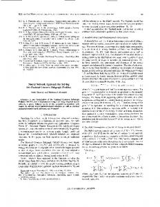
23
−0.06 0.1 −0.1
0.04
X4
−0.04 0.1 −0.1
0.04
X5
0.1
−0.04 −0.1
X1
0.1
−0.04 −0.1
−0.04 -0.1
0.1
X2
0.1
X4
0.1
−0.04 −0.1
−0.04 −0.1
X3
0.1
X6
0.1
0.04
0.04
0.04
X6
phi3
phi2
phi1 −0.04 −0.1
0.1
Y6
Y4 −0.3 −0.1
X3
0.04
phi6
X2
Y5
0.2
−0.05 0.1 −0.1
Y3
Y2 X1
phi4
−0.1
after NMC 0.04
0.04
0.06
0.15
Y1 −0.02
(b)
before NMC
0.08
phi5
(a)
X5
0.1
−0.04 -0.1
Figure 3: (a) Relationships among latent jointly Gaussian variables Xi and their nonlinear observations Yi . (b) Relationships among latent jointly Gaussian variables and inferred transformations using the NMC optimization. zero. We observe Yi = fi (Xi ) where, ⎧ ⎪ ⎪10X1 , Y1 = f1 (X1 ) = ⎨ 1 ⎪ ⎪ ⎩ 10 X1 , Y2 = f2 (X2 ) = e20X2 ,
if X1 ≥ 0, otherwise,
(6.9)
Y3 = f3 (X3 ) = −X3 , Y4 = f4 (X4 ) = X43 , ⎧ ⎪ ⎪e20X5 , Y5 = f5 (X5 ) = ⎨ −20X 5 ⎪ , ⎪ ⎩−e Y6 = f6 (X6 ) = X65 .
if X5 ≥ 0, otherwise,
The functions fi (⋅) remain unknown for the inference part. Relationships among original, observed and NMC variables are depicted in Figure 3. Then, we use φ∗i (Yi ) to infer the underlying covariance and precision matrices according to Theorem 11. As it is illustrated in Figure 4, covariance and precision matrices computed using observed variables Yi show significant errors compared to the true networks owing to the existence of extensive nonlinear relationships. However, inferred covariance and precision matrices using the NMC optimization closely approximate the true covariance and precision matrices, respectively (Theorem 11). Small errors in covariance coefficient estimation in this example are owing to computation of the NMC solution using empirical distributions according to the ACE algorithm 3.
24
(a)
before NMC
(b)
after NMC
before NMC
after NMC
1
1
1
1
2
2
2
2
3
3
3
3
4
4
4
4
5
5
5
5
6
6 1 0
2
3
4
5
error
6
6 1
2
3
4
5
6
6
1
0.7
0
2
3
4
5
error
6
1
2
3
4
5
6
1.2
Figure 4: For six nonlinear functions of jointly Gaussian variables described in Example 5, panel (a) plots covariance matrix errors before and after NMC. Using NMC, estimated covariance coefficients among variables are close to true ones. Panel (b) plots precision matrix errors before and after NMC. Using NMC, estimated elements of the precision matrix are close to true ones.
7
NMC Application in Inference of Nonlinear Relevance Graphs
Relevance graphs (RG’s) play an important role in many applications including systems biology, social and economic sciences as they characterize variable pairs with highest observed similarities [29]. Let X1 ,...,Xn be n random variables with zero means and unit variances. Consider a similarity measure S(Xi , Xj ) between variables Xi and Xj . If the similarity measure between variables Xi and Xj is independent of other variables, the resulting graph is called a pairwise relevance graph (PRG). Definition 8 Consider the following optimization: G∗S = arg max
∑ S(Xi , Xj ).
G=(V,E) (i,j)∈E ∣E∣=k
(7.1)
Then, G∗S = (V, E ∗ ) is called a pairwise relevance graph (PRG) of variables X1 , ..., Xn , with k edges, corresponding to the similarity measure S(⋅, ⋅). PRG’s can be inferred efficiently in practice. In the following, we highlight two examples of such graphs: Example 6 If S(⋅, ⋅) is a correlation-based similarity measure (e.g., S(Xi , Xj ) = ∣E[Xi Xj ]∣), the optimization (7.1) results in a correlation-based PRG. This graph only captures the top k linear associations among variables, ignoring nonlinear ones. Example 7 If S(⋅, ⋅) is a mutual information-based similarity measure (i.e., S(Xi , Xj ) = I(Xi ; Xj ) where I(.; .) represents the mutual information function [5]), optimization (7.1) results in an MIbased PRG which captures nonlinear associations among pairs of variables. However, it does not provide explicit forms of such nonlinear relationships. 25
Algorithm 4 Inference of a global relevance graph using NMC Input: X1 , . . . , Xn Initialization: E = {}, F1∗ = F1 , . . . , Fn∗ = Fn for r = 1 ∶ k do let {i, j, φ∗i , φ∗j } = argmaxE[φi′ (Xi′ )φj ′ (Xj ′ )] subject to: {i′ , j ′ } ∈ G × G ∖ E, φi′ ∈ Fi∗′ , φj ′ ∈ Fj∗′ update graph: E = E ∪ {(i, j)} update: run Algorithm 3 on G For i ∈ E, let φ∗i be the output function update function sets: For i ∈ E let Fi∗ = {φ∗i } end for run Algorithm 3 on G to obtain ρG∗ (X1 , . . . , Xn ) Output: E, ρG∗ (X1 , . . . , Xn ), φ∗i (Xi ), . . . , φ∗n (Xn ) If the similarity measure depends on all variables, the resulting graph is called a global relevance graph (GRG). A global relevance graph can capture system level properties of observed dependencies among variables. However, inference of a GRG is computationally challenging in general. Below, we introduce an NMC-based global relevance graph that captures observed nonlinear associations among variables and also provides explicit nonlinear transformation functions through which variables are associated. Definition 9 The NMC-based GRG of variables X1 , ..., Xn , with k edges is defined as G∗N M C = arg max
G=(V,E) ∣E∣=k
ρG (X1 , . . . , Xn ),
(7.2)
where ρG is defined in (4.1). Optimization (7.2) is combinatorial since it requires computation of NMC over all graphs with k edges. However, unlike MI-based GRG’s, the required sample size to have a reliable computation of G∗N M C does not increase with the size of the network. Below, we propose a greedy algorithm to find an approximate solution for optimization (7.2). Suppose at iteration r, the inferred network is G = (V, E) whose nodes are assigned to transformations φri . At this iteration, for each nonconnected pair of nodes, we wish to add the corresponding edge to the network, compute NMC, and finally select the edge with the highest NMC increase. However, this is computationally expensive as it requires NMC computation multiple times. Instead, at this iteration, we add an edge to the network with the highest correlation of its node transformations inferred in the last iteration. Then, we update all transformation functions by applying the ACE algorithm 3. We repeat this procedure explained in Algorithm 4 till the inferred network has a certain number of edges. Algorithm 4 starts from a graph with no edge and gradually populates it until the inferred graph has k edges. Alternatively, one can start with a complete graph and remove interactions with lowest nonlinear correlations iteratively. Because NMC is more efficient to run over sparse graphs (Proposition 7), the former has lower computational complexity than the later.
26
Nonlinear gene module inferred by NMC
Linear associations of inferred module
(b)
Breast Cancer (BRCA1)
Estimated survival functions
(a)
Survival time analysis 1
0.6
0.4
0.2
0 0
0
Time
Linear associations of inferred module
Group 1 Group 2
0.8
0.6
0.4
0.2
0
1
Survival time analysis
1
Estimated survival functions
Glioma Cancer (GBMLGG)
500 1000 1500 2000 2500 3000 3500 4000
1 Nonlinear gene module inferred by NMC
0
Group 1 Group 2
0.8
0
500 1000 1500 2000 2500 3000 3500 4000
Time
Figure 5: (a) Examples of nonlinear gene modules defined in Section 8, as a group of genes that is enriched in the NMC network but not in the linear one. (b) Survival time plots for corresponding nonlinear cancer modules of panel (a). For each inferred nonlinear cancer module, we partition individuals to two equal-size groups based on their average gene expression ranks in that module. We then perform a standard survival time analysis for each module and compute its associated log-rank p-value to determine its association with individual survival times in the considered cancer type.
8
Inference of Nonlinear Gene Modules in Cancer
Cancer is a complex disease involving abnormal cell growth with the potential to invade or spread to other parts of the body [44]. Different studies have shown associations of micro RNA patterns in different human cancers [30, 45]. In this section, we use NMC algorithms to infer gene modules of different cancer types that are detected over the nonlinear association network and not in the linear one. To perform these experiments, we use normalized RNA sequence counts from TCGA data portal for 24 cancer types at the gene level. We use processed the data provided in reference [30]. For each cancer type, first we select top 500 highly-variant genes based on their normalized variances [46]. Then, for each cancer, we compute both linear and nonlinear associations among genes. To compute NMC, we assume that conditions of Theorem 9 holds. That is, we assume that input data comes from, possibly nonlinear, functions of some latent jointly Gaussian variables satisfying conditions of Theorem 9. These functions are unknown and bijective. In general, this assumption is less restrictive than the assumption that input variables are jointly Gaussian. In this application, we wish to infer the strength of associations among genes in different cancers.
27
Nonlinear gene module inferred by NMC
Linear associations of inferred module
(b)
Survival time analysis 1
Estimated survival functions
Liver Cancer (LIHC)
(a)
0.6
0.4
0.2
0
0
1 Nonlinear gene module inferred by NMC
Linear associations of inferred module
0
1
1000
1500
Time
2000
2500
3000
Survival time analysis Group 1 Group 2
0.8
0.6
0.4
0.2
0 0
0
500
1
Estimated survival functions
Kidney Cancer (KIPAN)
Group 1 Group 2
0.8
500
1000
1500
Time
2000
2500
Figure 6: (a) Examples of nonlinear gene modules defined in Section 8, as a group of genes that is enriched in the NMC network but not in the linear one. (b) Survival time plots for corresponding nonlinear cancer modules of panel (a). For each inferred nonlinear cancer module, we partition individuals to two equal-size groups based on their average gene expression ranks in that module. We then perform a standard survival time analysis for each module and compute its associated log-rank p-value to determine its association with individual survival times in the considered cancer type. To compute an NMC association network, according to Note 2, we compute multiple MC’s among gene pairs using Algorithm 1. Moreover, we infer a linear association network by computing all pairwise correlations among gene expressions. We then select 5% of interactions among genes in the NMC network with largest nonlinear association increases compared to their linear association strengths. To have the same linear and nonlinear network densities, we select top 5% of interactions in the linear association network as well. Next, we partition each network to k groups using a standard spectral clustering algorithm based on the modularity transformation [47]. We use k = 10 in all cases as it leads to dense and large clusters. We define a gene module as a group of genes that are densely connected to each other in the network. We compute a p-value for each gene module in the network by permuting the network structure and comparing the density of the module in the original network with the ones in permutated networks. We only consider gene modules with p-values less than 0.05. A gene module is called nonlinear if it is present in the NMC network but not in the linear one. Figures 5 and 6 demonstrate examples of inferred nonlinear gene modules in different cancer types. For each inferred nonlinear module in a cancer type, we partition individuals to two equal-size 28
groups based on their average gene expression ranks in that module. We then perform a standard survival time analysis for each module based on Kaplan-Meier procedure to estimate survival function [48], and compute its associated log-rank p-value to determine its association with individual survival times in the considered cancer type [49]. We perform Benjamini and Hochberg multiple hypothesis correction [50] over the computed p-values of different nonlinear modules. For nonlinear modules with corrected p-values less than 0.05, we do further permutation analysis as follows: we randomly select the same number of genes as in the considered module, and compute its associated survival time p-value. If the corrected p-value of the nonlinear module is less than p-values of permutated modules at least in 95% of cases, we declare that nonlinear module as significantly associated with individual survival times in that cancer type. Figures 5 and 6 illustrate examples of nonlinear gene modules for Breast Cancer (BRCA1), Glioma Cancer (GBMLGG), Liver Cancer (LIHC), and Kidney Cancer (KIPAN). These gene modules are significantly associated with survival times of individuals while they are not detected using linear association measures. Several references [51–55] have hypothesized that complex nonlinear relationships among genes may play important roles in cancer pathways. Our proposed NMC algorithms and inferred nonlinear gene modules can be used in discovering such complex nonlinear relationships in different cancer types. However, further experiments should be performed to determine the involvement of these nonlinear gene modules in different cancers, which is beyond the scope of this paper.
9
Conclusion
In this paper, we proposed Network Maximal Correlation (NMC) as a fundamental measure to capture nonlinear associations over networks without the knowledge of underlying nonlinearity shapes. We showed that NMC extends the standard Maximal Correlation to the case of having large number of variables, by assigning each variable to a single transformation function, thus avoiding over-fitting issues of using multiple MC optimizations over network edges. We also introduced a regularized NMC optimization which penalizes total distances of inferred nonlinear transformations from original variables. One can use other standard regularization techniques to further restrict inferred nonlinear functions in practical applications. One of the main contributions of this work is providing a unifying framework to compute NMC (and therefore, MC) for both discrete and continuous variables using projections over appropriate Hilbert spaces. Using this framework, we established a connection between the NMC optimization with the MCP and MEP for discrete random variables, and with the Max-Cut problem for jointly Gaussian variables. Using these relationships, we provided efficient algorithms to compute NMC in different cases. To compute NMC for continuous random variables with general distributions, one can use the proposed optimization framework by choosing appropriate orthonormal basis for Hilbert spaces. For example, we used projections over Hermitte-Chebychev polynomials to characterize an optimal solution of the NMC optimization for jointly Gaussian variables. Compared to other nonlinear association measures such as mutual information (MI), NMC has two main advantageous: first, unlike MI-based measures that only compute the strength of associations among variables, NMC characterizes nonlinear transformation functions through which variables are related to each other. These inferred, possibly nonlinear, functions can be used in different applications such as regression. As an example, a nonlinear regression framework [56] can be efficiently designed using transformations of variables. Second, for the case of having large number 29
of variables, a reliable computation of conditional MI requires an excessive number of samples which often is not available in practice. Here, we showed that NMC can be reliably computed in practice and provided a finite sample generalization bound and error guarantees. NMC can be used in different areas to characterize nonlinear relationships, modules, and pathways among variables. Here, as an example, we applied NMC to different cancer datasets including breast, kidney and liver cancers, and showed that using NMC networks, we can infer nonlinear gene modules that are not detectable using linear association measures while they are significantly associated with survival times of individuals. Similarly, NMC can be applied to infer nonlinear gene interactions, modules and pathways in different types of biological networks such as regulatory [57] and PPI [58] networks. Moreover, NMC can be used over social/economic networks to characterize belief/behaviour variations of individuals/entities through their interactions over the underlying networks [59]. We believe that the proposed NMC framework and algorithms can make a significant impact in many areas of network sciences, statistics, information theory, systems biology, social sciences, and beyond.
10 10.1
Proofs Proof of Proposition 1
∞ Let {ψ1,i }∞ i=1 and {ψ2,i }i=1 be the corresponding orthonormal bases of H1 and H2 in Definition 2. We can represent functions φ1 (X1 ) and φ2 (X2 ) in terms of the basis functions as follows: ∞
φ1 (x1 ) = ∑ a1,i ψ1,i (x1 ), i=1 ∞
φ2 (x2 ) = ∑ a2,i ψ2,i (x2 ), i=1
2 ∞ for two sequence of coefficients {a1,i }∞ i=1 and {a2,i }i=1 . Thus, the constraint E[φi (Xi ) ] = 1 in opti∞ 2 mization (2.1) would be translated into ∑j=1 ai,j = 1 and the constraint E[φi (Xi )] = 0 is simplified to ∑∞ j=1 ai,j E[ψi,j (Xi )] = 0, for i = 1, 2. Moreover, we have ∞
E[φ1 (X1 )φ2 (X2 )] = ∑ a1,i a2,j E[ψ1,i (X1 )ψ2,j (X2 )]. i,j=1
(10.1)
Thus, maximal correlation optimization (2.1) can be re-written as follows: min
∑ a1,i a2,j E[ψ1,i (X1 )ψ2,j (X2 )] i,j ∞
(10.2)
2 ∑ ai,j = 1, i = 1, 2,
j=1 ∞
∑ ai,j E[ψi,j (Xi )] = 0, i = 1, 2.
j=1
Moreover, {ψ1,i ψ2,j }i,j forms a basis for co-variate L2 functions of X1 and X2 including the joint distribution function PX1 X2 (⋅, ⋅). Therefore, we have PX1 X2 (x1 , x2 ) = ∑ ρij ψ1,i (x1 )ψ2,j (x2 ). i,j
30
(10.3)
Using equation (10.3), we have ρij = E[ψ1,i (X1 )ψ2,j (X2 )].
(10.4)
Using (10.4) in optimization (10.2) leads to optimization (2.2). This completes the proof.
10.2
Proof of Theorem 1
We use the following lemma in the proof of Theorem 1. Lemma 2 (a) Let P and P˜ be the matrix form of two joint probability distribution on (X1 , X2 ), such that PX1 ,X2 (x1 , x2 ) = [P ]x1 ,x2 and P˜X1 ,X2 (x1 , x2 ) = [P˜ ]x1 ,x2 . We bound the difference ˜ by the difference between P and P˜ , as follows: between Q and Q, ˜ = ∣∣DX (P )− 21 P DX (P )− 12 − DX (P˜ )− 12 P˜ DX (P˜ )− 12 ∣∣ ≤ ∣∣Q − Q∣∣ 2 2 1 1 2 2 1 1 1 1 1 √ ∣∣P ∣∣2 ∣∣DX2 (P )− 2 − DX2 (P˜ )− 2 ∣∣2 + √ ∣∣P − P˜ ∣∣2 √ δX1 (P ) δX1 (P ) δX (P˜ ) 2
+√
1 δX2 (P˜ )
∣∣P˜ ∣∣2 ∣∣DX1 (P )
− 12
− DX1 (P˜ )
− 12
∣∣2 .
(10.5)
(b) Furthermore, we have √ √ 1 1 1 ˜ 2≤√ 1 ∣∣Q − Q∣∣ D∣∣DX2 (P ) − DX2 (P˜ )∣∣∞ D∣∣P − P˜ ∣∣∞ +√ √ 2δX2 (P, P˜ )3 δX1 (P ) δX1 (P ) δX (P˜ ) 2 √ 1 1 +√ D∣∣DX1 (P ) − DX1 (P˜ )∣∣∞ , (10.6) 2δX2 (P, P˜ )3/2 ˜ δX2 (P ) where D = max{∣X1 ∣, ∣X2 ∣},δX2 (P, P˜ ) = min{δX2 (P ), δX2 (P˜ )}, and δX1 (P, P˜ ) = min{δX1 (P ), δX1 (P˜ )}. Proof We have ˜ 2 ≤ ∣∣DX (P )− 21 P DX (P )− 21 − DX (P˜ )− 12 P˜ DX (P˜ )− 12 ∣∣ ≤ ∣∣Q − Q∣∣ 2 1 2 1 2 1 1 1 1 ∣∣DX1 (P )− 2 P DX2 (P )− 2 − DX1 (P )− 2 P DX2 (P˜ )− 2 1 1 1 1 + DX1 (P )− 2 P DX2 (P˜ )− 2 − DX1 (P˜ )− 2 P˜ DX2 (P˜ )− 2 ∣∣2 ≤ 1 1 1 1 1 1 ∣∣DX1 (P )− 2 P ∣∣2 ∣∣DX2 (P )− 2 − DX2 (P˜ )− 2 ∣∣2 + ∣∣DX2 (P˜ )− 2 ∣∣2 ∣∣DX1 (P )− 2 P − DX1 (P˜ )− 2 P˜ ∣∣2 ≤ 1 1 1 ∣∣DX1 (P )− 2 P ∣∣2 ∣∣DX2 (P )− 2 − DX2 (P˜ )− 2 ∣∣2 + 1
1
1
1
1
∣∣DX2 (P˜ )− 2 ∣∣2 ∣∣DX1 (P )− 2 P − DX1 (P )− 2 P˜ + DX1 (P )− 2 P˜ − DX1 (P˜ )− 2 P˜ ∣∣2 ≤ 1
1
1
1
1
∣∣DX1 (P )− 2 P ∣∣2 ∣∣DX2 (P )− 2 − DX2 (P˜ )− 2 ∣∣2 + ∣∣DX2 (P˜ )− 2 ∣∣2 ∣∣DX1 (P )− 2 ∣∣2 ∣∣P − P˜ ∣∣2 + 1
1
1
∣∣DX2 (P˜ )− 2 ∣∣2 ∣∣P˜ ∣∣2 ∣∣DX1 (P )− 2 − DX1 (P˜ )− 2 ∣∣2 .
(10.7)
For any distribution PX1 ,X2 (⋅, ⋅), we have 1
∣∣DX1 (P )− 2 ∣∣2 = max √ X1 ∈X1
31
1 PX1 (X1 )
=√
1 δX1 (P )
(10.8)
and 1 1 1 ∣∣DX2 (P )− 2 ∣∣2 = max √ =√ . X2 ∈X2 PX2 (X2 ) δX2 (P )
(10.9)
By substituting (10.8) and (10.9) in (10.7), we obtain ˜ 2≤√ ∣∣Q − Q∣∣
1 δX1 (P )
+√
1 δX2 (P˜ )
1
1
∣∣P ∣∣2 ∣∣DX2 (P )− 2 − DX2 (P˜ )− 2 ∣∣2 + √ 1
1 δX1 (P )
√
1 δX2 (P˜ )
∣∣P − P˜ ∣∣2
1
∣∣P˜ ∣∣2 ∣∣DX1 (P )− 2 − DX1 (P˜ )− 2 ∣∣2 .
(10.10)
This completes the first part of the lemma. Furthermore, for a joint probability distribution matrix P (⋅, ⋅), we have ∣∣P ∣∣∞ ≤ 1 and ∣∣P ∣∣1 ≤ 1. Moreover, we have Lemma 3 For a given m × n matrix, A, we have √ ∣∣A∣∣2 ≤ m∣∣A∣∣∞ , and ∣∣A∣∣2 ≤ Therefore, using Lemma 3, we have ∣∣P ∣∣2 ≤ Using this, we obtain the following: ˜ 2≤√ ∣∣Q − Q∣∣
1 δX1 (P ) 1
√
√ n∣∣A∣∣1 .
∣X2 ∣∣∣P ∣∣1 ≤
√ D∣∣DX2 (P ) − DX2 (P˜ )∣∣∞
√
∣X2 ∣ and ∣∣P ∣∣2 ≤
√
∣X1 ∣∣∣P ∣∣∞ ≤
√
∣X1 ∣.
√ 1 1 1 +√ D∣∣P − P˜ ∣∣∞ √ 2δX2 (P, P˜ )3 δX1 (P ) δX (P˜ ) 2
√
1 D∣∣DX1 (P ) − DX1 (P˜ )∣∣1 , +√ 2δX1 (P, P˜ )3/2 δX2 (P˜ )
(10.11)
where D = max{∣X1 ∣, ∣X2 ∣}, δX2 (P, P˜ ) = min{δX2 (P ), δX2 (P˜ )}, and δX1 (P, P˜ ) = min{δX1 (P ), δX1 (P˜ )}. This concludes the proof. ˜ be the corresponding normalized distribution matrices of P Now we prove Theorem 1. Let Q and Q ˜ and P , respectively. Suppose the joint distribution on (X1 , X2 ) is according to P . Using Example 2, we have ρ(X1 , X2 ) = σ2 , where σ2 is the second largest singular value of the matrix Q. Similarly, maximal correlation under the joint distribution P˜ is σ ˜2 , where σ ˜2 is the second largest singular ˜ Moreover, we have value of the matrix Q. Theorem 12 Let A1 and A2 be two matrices of the same size. We have (1)
∣σi
(2)
− σi ∣ ≤ ∣∣A1 − A2 ∣∣2 ,
where σi1 and σi2 are the i-th largest singular values of A1 and A2 , respectively.
32
(10.12)
Proof See e.g. reference [60]. Using Theorem 12 and part (a) of Lemma 2, we have ˜ 2≤√ ∣σ2 − σ ˜2 ∣ ≤ ∣∣Q − Q∣∣
1
1 1 1 1 ∣∣P ∣∣2 ∣∣DX2 (P )− 2 − DX2 (P˜ )− 2 ∣∣2 + √ ∣∣P − P˜ ∣∣2 √ δX1 (P ) δX1 (P ) δX (P˜ ) 2
+√
1 δX2 (P˜ )
∣∣P˜ ∣∣2 ∣∣DX1 (P )
− 21
− DX1 (P˜ )
− 21
∣∣2 .
(10.13)
Furthermore, using part (b) of Lemma 2, we have ∣σ2 − σ ˜2 ∣ ≤ √
1 δX1 (P ) 1
√ D∣∣DX2 (P ) − DX2 (P˜ )∣∣∞
√ 1 1 1 D∣∣P − P˜ ∣∣∞ +√ √ 2δX2 (P, P˜ )3/2 δX1 (P ) δX (P˜ ) 2
√
1 +√ D∣∣DX1 (P ) − DX1 (P˜ )∣∣∞ . 2δX2 (P, P˜ )3/2 δX2 (P˜ )
(10.14)
Let δ = min{δX1 (P ), δX1 (P˜ ), δX2 (P ), δX2 (P˜ )} and D = max{∣X1 ∣, ∣X2 ∣}. Since, ∣∣P − P˜ ∣∣∞ ≤ �, we have � √ �√ � √ � √ ∣σ2 − σ ˜2 ∣ ≤ 2 D D + D + 2 D D ≤ 2 2 D D. (10.15) 2δ δ 2δ δ This completes the proof.
10.3
Proof of Theorem 2
Using Lemma 2 and union bound, we have
P [∣σ2 (Qm ) − σ2 (Q)∣ > �] ≤ P[
1 1 1 � ∣∣DX2 (P (m) )− 2 − DX2 (P )− 2 ∣∣2 ∣∣P ∣∣2 > ] δX1 (P ) 3
+ P[
1 1 � ∣∣P (m) − P ∣∣2 > ] (m) δX1 (P ) δX2 (P 3 )
+ P[
1 1 1 � ∣∣DX1 (P (m) )− 2 − DX1 (P )− 2 ∣∣2 ∣∣P (m) ∣∣2 > ] (m) 3 δX2 (P )
1 1 � 1 ≤ P [∣∣DX2 (P (m) )− 2 − DX2 (P )− 2 ∣∣∞ > δX1 (P ) √ ] 3 D
� 1 + P [∣∣P (m) − P ∣∣∞ > δX1 (P )δX2 (P (m) ) √ ] 3 D 1 1 � 1 + P [∣∣DX1 (P (m) )− 2 − DX1 (P )− 2 ∣∣∞ > δY (P (m) ) √ ] 3 D
where D = max{∣X1 ∣, ∣X2 ∣}. Moreover, we have 33
(10.16)
Theorem 13 Let P be a probability distribution over alphabets X . Also, let P (m) denote the empirical probability distribution of X, obtained from m i.i.d. samples, {xi }m i=1 , drawn according to P . We have 2
P [∣∣P (m) − P ∣∣∞ > �] ≤ 4e−m� .
(10.17)
Proof See e.g. references [61, 62]. Using Theorem 13, we have 1 2
1
2
P [∣∣P (m) (X2 ) − P (X2 )∣∣ ≥ δX2 (P )] ≤ 4e−m( 2 δX2 (P )) . This occurs with probability less than η/2 if m ≥ 1 2 δX2 (P ),
1 − log η/2 4 ( 1 δ)2 . 2
Moreover, given ∣∣P (m) (X2 ) − P (X2 )∣∣ ≥
we obtain δX2 (P (m) ) > 21 δX2 (P ). We also have
P [∣σ2 (Qm ) − σ2 (Q)∣ > �]
1 1 = P [∣σ2 (Qm ) − σ2 (Q)∣ > � ∣ ∣∣P (m) (X2 ) − P (X2 )∣∣ ≥ δX2 (P )] P [∣∣P (m) (X2 ) − P (X2 )∣∣ ≥ δX2 (P )] 2 2 1 1 + P [∣σ2 (Qm ) − σ2 (Q)∣ > � ∣ ∣∣P (m) (X2 ) − P (X2 )∣∣ ≤ δX2 (P )] P [∣∣P (m) (X2 ) − P (X2 )∣∣ ≤ δY (P )] 2 2 1 1 ≤ P [∣σ2 (Qm ) − σ2 (Q)∣ > � ∣ ∣∣P (m) (X2 ) − P (X2 )∣∣ ≤ δY (P )] + P [∣∣P (m) (X2 ) − P (X2 )∣∣ ≥ δX2 (P )] . 2 2
Let m ≥
η
1 − log 2 4 ( 1 δ)2 2
to make the second term less than or equal to 12 η. Next, we choose m sufficiently
large so that the first term is no greater than 21 η. Using (10.16), we have 1 2
P [∣σ2 (Qm ) − σ2 (Q)∣ > � ∣ ∣∣P (m) (X2 ) − P (X2 )∣∣ ≤ δX2 (P )] ≤ P [∣∣DX2 (P (m) ) − DX2 (P )∣∣∞ >
1 � (2δX2 (P )3 ) δX1 (P ) √ ] 3 D
1 � 1 + P [∣∣P (m) − P ∣∣∞ > δX1 (P ) δX2 (P ) √ ] 2 3 D 1 � 1 + P [∣∣DX1 (P (m) ) − DX1 (P )∣∣∞ > (2δX1 (P )3 ) δX2 (P ) √ ] . 2 3 D Now using Theorem 13, each term on the righthand side goes to zero exponentially fast. Moreover, 2 we have P[∣σ2 (Qm ) − σ2 (Q)∣ > �] ≤ 12e−me , where � 1 1 � 1 1 � 1 e = min{ (2δX2 (P )3 ) δX1 (P ) √ , δX (P ) δX2 (P ) √ , (2δX1 (P )3 ) δX2 (P ) √ }, 3 2 3 D 2 3 D D which is equal to 3� δ 4 √1 . Therefore, in order to have P[∣σ2 (Qm )−σ2 (Q)∣ > � ∣ ∣∣P (m) (X2 )−P (X2 )∣∣ ≤ 1 2 δX2 (P )]
D
≤ η2 , it suffices to have
m≥ Therefore, overall it suffices to have m ≥
log 24 η � 4 √1 δ 3 D
log 12 η 2
� 4 √1 3δ D
.
. This concludes the proof. 34
10.4
Proof of Lemma 1
Consider the following MSE optimization. We have min
φ1 ,...,φn
1 2 ∑ E[(φi (Xi ) − φj (Xj )) ] 2 (i,j)∈E ∑ E[φi (Xi )φj (Xj )].
=∣E∣ − max
φ1 ,...,φn
(i,j)∈E
Therefore, the NMC optimization (4.1) is equivalent to the following MSE optimization: 1 2 ∑ E[(φi (Xi ) − φj (Xj )) ], 2 (i,j)∈E
min
φ1 ,...,φn
(10.18)
where E[φi (Xi )] = 0 and E[φ2i (Xi )] = 1, for any 1 ≤ i ≤ n.
10.5
Proof of Proposition 2
Let Fi = {φi ∈ Hi ∶
E[φi ] = 0, E[φ2i ] = 1} .
Now consider the function defined on F1 × ⋅ ⋅ ⋅ × Fn , as R(φ1 , . . . , φn ) = ∑ E[φi (Xi )φj (Xj )]. (i,j)∈E
Below, we show that R is continuous and F1 × ⋅ ⋅ ⋅ × Fn is a compact subset of a finite dimensional space. For any 1 ≤ i ≤ n, first we show Fi is compact. Since Fi is a subset of compact space Hi , it suffices to show that it is closed. This evidently follows from the definition of the norm on Hi , which is √ E[(φi − φ′i )2 ]. Since F1 × ⋅ ⋅ ⋅ × Fn is the product of finitely many compact sets, therefore, it is compact as well. Next we show R is continuous. Since R has finitely many arguments, it suffices to show that it is continuous with respect to each argument. Let 1 ≤ i0 ≤ n. We have R(φ1 , . . . , φn ) =
∑
j∈N (i0 )
= ⟨φi0 ,
⟨φi0 , Pi0 φj ⟩ + ∑
j∈N (i0 )
Pi0 φj ⟩ +
∑
⟨φi , φj ⟩
∑
⟨φi , φj ⟩ ,
(i,j)∈E, i≠i0 , j≠i0
(i,j)∈E, i≠i0 , j≠i0
where Pi denotes the projection operation from the space Hj (for any j ≠ i) onto Hi . Moreover, we can employ on Weierstrass Extreme Value Theorem that says every continuous real-valued function on a compact space attains its extreme values. Since ⟨φi0 , ∑j∈N (i0 ) Pi0 φj ⟩ is continuous with respect to φi0 , the function R ∶ F1 × ⋅ ⋅ ⋅ × Fn → R is continuous. Thus, function R attains its maximum on F1 × ⋅ ⋅ ⋅ × Fn , which complete the proof.
35
10.6
Proof of Proposition 3
For a given 1 ≤ i0 ≤ n, we have ∑ ⟨φi , φj ⟩ =
(i,j)∈E
∑
j∈N (i0 )
= ⟨φi0 , ≤ ∣∣
⟨φi0 , Pi0 φj ⟩ + ∑
j∈N (i0 )
∑
j∈N (i0 )
Pi0 φj ⟩ +
Pi0 φj ∣∣ +
∑
⟨φi , φj ⟩
∑
⟨φi , φj ⟩
(i,j)∈E, i≠i0 , j≠i0
(i,j)∈E, i≠i0 , j≠i0
∑
(i,j)∈E, i≠i0 , j≠i0
⟨φi , φj ⟩ ,
where the last inequality that follows from Cauchy-Schwartz inequality becomes an equality if and only if we have φ∗i0 = c ∑j∈N (i0 ) Pi0 φ∗j , for some constant c > 0. Since we have ∣∣φ∗i0 ∣∣ = 1, we obtain φ∗i0 =
∑j∈N (i0 ) Pi0 φ∗j , ∣∣ ∑j∈N (i0 ) Pi0 φ∗j ∣∣
which completes the proof.
10.7
Proof of Theorem 3
Since any Hilbert space has an orthonormal basis (Theorem 2.4, [33]), let {ψi,j }∞ j=1 be the corresponding orthonormal basis of Hi for 1 ≤ i ≤ n. Therefore, we can represent φi (Xi ) in terms of the basis as follows: ∞
φi (xi ) = ∑ ai,j ψi,j (xi ). j=1
2 The constraint E[φi (Xi )2 ] = 1 translates into ∑∞ j=1 ai,j = 1 and the constraint E[φi (Xi )] = 0 trans∞ lates into ∑j=1 ai,j E[ψi,j (Xi )] = 0 for 1 ≤ i ≤ n. Moreover, for any i and i′ we have
E[φi (Xi )φi′ (Xi′ )] = ∑ ai,j ai′ ,j ′ E[ψi,j (Xi )ψi′ ,j ′ (Xi′ )], j,j ′
The network maximal correlation can be found by solving the following optimization problem. max
∑ ∑ ai,j ai′ ,j ′ E[ψi,j (Xi )ψi′ ,j ′ (Xi′ )]
(i,i′ )∈E j,j ′ ∞ 2 ∑ ai,j = 1, j=1 ∞
1 ≤ i ≤ n,
∑ ai,j E[ψi,j (Xi )] = 0, 1 ≤ i ≤ n,
j=1
Moreover, since {ψi,j ψi′ ,j ′ } is a basis for functions of Xi and Xi′ (with the corresponding inner product), we can write the joint density function as ′ ′ ′ PXi Xi′ (Xi , Xi′ ) = ∑ ρj,j i,i′ ψi,j (Xi )ψi ,j (Xi ). ′
j,j ′
Using this equation, we have E[ψi,j (Xi )ψi′ ,j ′ (Xi′ )] = ρj,j i,i′ , which completes the proof. ′
36
10.8
Proof of Theorem 4
Let P and P˜ be two distributions over (X1 , . . . , Xn ). We shall compare the solution of the two following optimization problems. max ai
T ∑ ai Qi,i′ ai
(10.19)
(i,i′ )∈E
∣∣ai ∣∣2 = 1, √ ai ⊥ pi ,
1 ≤ i ≤ n, 1 ≤ i ≤ n,
and max ai
T ˜ ∑ ai Q i,i′ ai
(10.20)
(i,i′ )∈E
∣∣ai ∣∣2 = 1, √ ˜ i, ai ⊥ p
1 ≤ i ≤ n, 1 ≤ i ≤ n.
Let ρG and ρ˜G be the optimal solution for (10.19) and (10.20), respectively. For any (i, j) ∈ E, suppose ∣∣P − P˜ ∣∣∞ ≤ �. Also, suppose δ = min1≤i≤n (min{δXi (PXi ), δXi (P˜Xi )}). Let the optimal solution of optimization (10.19) be a∗i . Based on this solution, we shall construct a feasible solution for optimization (10.20) and then evaluate its objective function. For any i, let √ √ √ ˜ i < a∗i , pi − p ˜ i >) (a∗i + p √ bi = ∗ √ . √ ∗ ˜ i < ai , pi − p ˜ i > ∣∣ ∣∣ai + p We claim this set of vectors is feasible for optimization√(10.20). First note that the norm of each ˜ i. bi is one. We next show that each bi is orthogonal to p < bi ,
√
˜ i >= p
∣∣a∗i
+
√
1
˜i < p
√ a∗i , pi
√ (< a∗i , ˜ i > ∣∣ − p
√ √ √ √ ˜ i > + < a∗i , pi − p ˜ i > ∣∣ p ˜ i ∣∣) = 0, p
√ ˜ i ∣∣ = 1. We now plug in the feasible solution bi into the where the last equality follows from ∣∣ p objective function of optimization (10.20). ρ˜G ≥
T ˜ ∑ bi Q ii′ bi′ =
(i,i′ )∈E
T ˜ T ∗T ∗T ∗ ∗T ∗ ∑ bi (Q ii′ − Qii′ ) bi′ + (bi − a i ) Qii′ bi′ + a i Qii′ (bi′ − ai′ ) + a i Qii′ ai′
(i,i′ )∈E
˜ ii′ − Qii′ ) bi′ + (bTi − a∗ Ti ) Qii′ bi′ + a∗ Ti Qii′ (bi′ − a∗i′ ) . = ρG + ∑ bTi (Q
(10.21)
(i,i′ )∈E
We now bound each term on the right hand side of equation (10.21). Using Lemma 2, for any i, i′ , we have ˜ ii′ − Qii′ ) bi′ ∣ ≤ ∣∣Q ˜ ii′ − Qii′ ∣∣2 ≤ 3 � D3/2 . ∣bTi (Q 2 δ2
37
We also have T
T
T
∣ (bTi − a∗ i ) Qii′ bi′ ∣ ≤ ∣∣bTi − a∗ i ∣∣2 ∣∣Qii′ ∣∣2 ∣∣bi′ ∣∣2 = ∣∣bTi − a∗ i ∣∣2 √ √ √ ˜ i < a∗i , pi − p ˜ i > ∣∣2 ∣∣ p √ √ ≤ √ ∗ ˜ i < a i , pi − p ˜ i > ∣∣2 1 − ∣∣ p √ √ √ √ √ ∗ √ ˜ i < ai , pi − p ˜ i > ∣∣2 ˜ i < a∗i , pi − p ˜ i > ∣∣2 ∣∣ p ∣∣ p √ √ √ √ + max{ , }, √ √ ˜ i < a∗i , pi − p ˜ i > ∣∣2 1 + ∣∣ p ˜ i < a∗i , pi − p ˜ i > ∣∣2 1 − ∣∣ p where we use the following basic inequality ∣∣
� 1 a+� − a∣∣2 = ∣∣ + a( − 1) ∣∣2 ∣∣a + �∣∣2 ∣∣a + �∣∣2 ∣∣a + �∣∣2 � 1 ≤ ∣∣ ∣∣2 + ∣∣a∣∣2 ∣ − 1∣ ∣∣a + �∣∣2 ∣∣a + �∣∣2 ∣∣�∣∣2 1 1 ≤ + max{∣ − 1∣, ∣ − 1∣}, 1 − ∣∣�∣∣2 1 − ∣∣�∣∣2 1 + ∣∣�∣∣2
where we used 1 − ∣∣�∣∣2 ≤ ∣∣a + �∣∣2 ≤ 1 + ∣∣�∣∣2 to obtain the last inequality. Therefore, we have √ √ √ ˜ i > ∣∣2 ∣∣ p˜i < a∗i , pi − p ∗T T √ . ∣ (bi − a i ) Qii′ bi′ ∣ ≤ 2 √ √ ∗ ˜ i > ∣∣2 1 − ∣∣ p˜i < ai , pi − p √ √ √ ˜ i < a∗i , pi − p ˜ i > ∣∣2 . Using Cauchy-Schwartz, we have We shall now bound the term ∣∣ p √ √ √ √ √ √ � ˜ i < a∗i , pi − p ˜ i > ∣∣2 ≤ ∣∣ p ˜ i ∣∣2 ∣∣a∗i ∣∣2 ∣∣ pi − p ˜ i > ∣∣2 ≤ 1/2 D3/2 , ∣∣ p 2δ √ √ ˜ i (j)∣ ≤ �D and ∣ p ˜ i (j)− pi (j)∣ ≤ ∣pi (j)− p ˜ i (j)∣ 2δ11/2 . Plugging where we use the fact that ∣pi (j)− p in this inequality and choosing � sufficiently small to guarantee 2δ�1/2 D3/2 ≤ 12 , we obtain T
∣ (bTi − a∗ i ) Qii′ bi′ ∣ ≤ 2
�
δ 1/2
D3/2 ,
which leads to ρ˜G ≥ ρG − ∑ 4 (i,i′ )∈E
� δ 1/2 4
3
= ρG − �∣E∣D 2 (
D3/2 +
δ 1/2
+
3� 3/2 D 2δ 2
3 ). 2δ 2
Similarly, we have ρG ≥ ρ˜G − ∑ 4 (i,i′ )∈E
3� � D3/2 + 2 D3/2 2δ δ 1/2 4
3
= ρG − �∣E∣D 2 (
δ 1/2
+
3 ). 2δ 2
Combining the previous two relations, we obtain 3
∣˜ ρG − ρG ∣ ≤ �∣E∣D 2 (
4 δ 1/2
which completes the proof. 38
+
3 6 3 ) ≤ �∣E∣D 2 2 , 2 2δ δ
10.9
Proof of Theorem 5
Using Theorem 13 for any (i, i′ ) ∈ E, we have 2
(m) −mγ P[∣∣Pi,i . ′ − Pi,i′ ∣∣∞ > γ] ≤ 4e
Therefore, using the union bound, we obtain (m) (m) P[∩(i,i′ )∈E 1{∣∣Pi,i ′ − Pi,i′ ∣∣∞ < γ}] = 1 − P[∪(i,i′ )∈E 1{∣∣Pi,i′ − Pi,i′ ∣∣∞ > γ}] 2
(m)
≥ 1 − ∑ P[1{∣∣Pi,i′ − Pi,i′ ∣∣∞ > γ}] ≥ 1 − 4∣E∣e−nγ . (i,i′ )∈E
On the other hand, we have δ 2
δ 2
(m) (m) P[δ(Pi(m) ) ≥ ] ≥ P[∣∣Pi(m) − Pi ∣∣∞ ≤ ] ≥ P[∣∣Pi,i ′ ∣ − Pi,i′ ∣∞ ≤ (m)
(m)
≥ 1 − P[∣∣Pi,i′ − Pi,i′ ∣∣∞ >
δ ] 2D
δ 2 δ ] ≥ 1 − 4e−m( 2D ) . 2D
Therefore, using the union bound, we obtain δ 2
δ
2
P[∩i∈V 1{δ(Pi(m) ) ≥ }] ≥ 1 − 4∣V ∣e−m( 2D ) . By applying the union bound once more, we have δ 2
δ
2
2
(m) (m) P[∩(i,i′ )∈E 1{∣∣Pi,i ) ≥ }] ≥ 1 − 4∣V ∣e−m( 2D ) − 4∣E∣e−mγ . ′ − Pi,i′ ∣∣∞ < γ} ∩i∈V 1{δ(Pi
Therefore, for a given η > 0 for m ≥ m0 , where n0 is the smallest solution of δ
2
2
η ≥ 4∣V ∣e−m( 2D ) + 4∣E∣e−mγ , with probability at least 1 − η, we have ∣ρm (G) − ρG ∣ ≤ γ∣E∣D3/2
24 . δ
We let ∣ρm (G) − ρG ∣ ≤ � and find γ as γ=
� δ −3/2 D . ∣E∣ 24
We plug this into the equation for m0 to find δ
2
η ≥ 4∣V ∣e−m( 2D ) + 4∣E∣e
2
� δ −m( ∣E∣ D−3/2 ) 24
.
This leads to m0 ≥
⎛ ⎞ 1 8 max{∣V ∣, ∣E∣} log ( ) δ 2 � δ −3/2 2 η ⎝ min{( 2D ⎠ ) , ( ∣E∣ 24 D ) }
≥(
24∣E∣2 D3 8 max{∣V ∣, ∣E∣} ) log ( ). 2 2 � δ η 39
10.10
Proof of Theorem 6
To prove Theorem 6, first we prove the following Lemma: Lemma 4 NMC optimization (4.1) can be written as follows: ∑ E[(φi − φ¯i )(φi′ − φ¯i′ )]
max
(i,i′ )∈E
(10.22)
(i,i′ )∈E
var (φi ) = 1,
1 ≤ i ≤ n,
where φ¯i and var (φi ) represent the mean and the variance of the random variable φi . Proof Denote the optimum value of optimization (10.22) by ρ˜G . Let φ∗i be an optimal solution of (4.1). The set of functions φ∗i for i = 1, . . . , n is feasible for optimization (10.22) and therefore we have ρG ≤ ρ˜G . On the other hand, let φ∗∗ i be an optimal solution of optimization (10.22). Let ∗∗ ∗∗ ˜ ¯ ˜ φi = φi − φi . The set of functions φi for i = 1, . . . , n is feasible for optimization (4.1). Thus, we have ρG ≥ ρ˜G . Therefore, we have that ρG = ρ˜G . √ Let ai = φi / pi . We have √ √ √ 1 = var(φi ) = E[φ2i ] − (E[φi ])2 = ∣∣ai ∣∣22 − (ai pi )2 = aTi (I − pi pi T ) ai . √ √ We next show that the matrix I − pi pi T is positive semidefinite and the only vectors in its null √ space is 0 and pi . This is because xT (I −
√ √ T √ pi pi ) x = ∣∣x∣∣22 − (x pi )2 ≥ 0,
(10.23)
√ where we use Cauchy-Schwartz and ∣∣ pi ∣∣22 = 1 to obtain the last inequality (10.23). This inequality √ becomes an equality if and only if x = 0 or x = pi . Now consider the objective function of optimization (10.22). We have
E[(φi − φ¯i )(φi′ − φ¯i′ )] = E[φi φi′ ] − φ¯i φ¯i′ = aTi Qii′ ai − (aTi
√
pi )(aTi′
√
pi′ ) = aTi (Qii′ −
√ √ T pi pi′ ) ai′ .
Therefore, optimization (10.22) (which is equivalent to the NMC optimization (4.1) according to Lemma 4) can be written as, max ai
T ∑ ai (Qii′ −
(i,i′ )∈E
aTi (I −
√ √ T pi pi′ ) ai′
√ √ T pi pi ) ai = 1,
(10.24)
1 ≤ i ≤ n.
√ √ √ √ For each i, since I − pi pi T is positive semidefinte. Thus, we can write I − pi pi T = Bi BiT . Let bi = Bi ai . Thus, constraints of optimization (10.24) can be written as bTi bi = ∣∣bi ∣∣22 = 1. We next write ai as a function of bi . Note that since Bi is not invertible, there are many choices for ai as a function of bi characterized as follows: Let Ui Σi UiT be the singular value decomposition √ (1) of Bi . The vector pi is the singular vector corresponding to singular value zero (σi = 0). (2)
(∣Xi )
ai = ([Ui , . . . , Ui
(ni )
]diag(1/σi2 , . . . , 1/σi
(2)
√ √ ] ) bi + αi pi = Ai bi + αi pi ,
(∣Xi ) T
)[Ui , . . . , Ui
(10.25) 40
(j)
(j)
where Ui is the j-th column of Ui , σi is the j-th singular value of Bi , and αi can be any scalar.3 Below, we show that all choices of ai according to (10.25) lead to the same objective function of optimization (10.24): √ √ √ √ aTi (Qii′ − pi pi′ T ) ai′ = bTi ATi (Qii′ − pi pi′ T ) Ai′ bi′ √ √ √ + bTi ATi (Qii′ − pi pi′ T ) αi′ pi′ √ √ √ + αi pi T (Qii′ − pi pi′ T ) Ai′ bi′ √ √ √ √ + αi pi T (Qii′ − pi pi′ T ) αi′ pi′ √ √ = bTi ATi (Qii′ − pi pi′ T ) Ai′ bi′ √ + bTi ATi Qii′ αi′ pi′ √ + αi pi T Qii′ Ai′ bi′ + αi αi′ (1 − 1)
√ √ = bTi ATi (Qii′ − pi pi′ T ) Ai′ bi′ √ + bTi ATi pi αi′ √ √ √ + αi pi′ T Ai′ bi′ = bTi ATi (Qii′ − pi pi′ T ) Ai′ bi′ . Therefore, the NMC optimization (4.1) can be written as √ √ T T T max ∑ bi Ai (Qii′ − pi pi′ ) Ai′ bi′ bi
(i,i′ )∈E
∣∣bi ∣∣2 = 1. This completes the proof.
10.11
Proof of Proposition 6
We use the following lemma in the proof of Proposition 6. Lemma 5 Let X and Y be two random variables such that E[X] = E[Y ] = 0. The solution to the optimization max φ
E[φ(X)Y ] E[φ(X)] = 0 E[φ(X)2 ] = 1,
is φ(X) = 3
E[Y ∣X] . E[(E[Y ∣X])2 ]
√
Since Bi is symmetric it has a set of ∣Xi ∣ orthonormal eigenvectors and can be written as ∣Xi ∣
Bi = ∑ vj σi vjT . (j)
j=1
Let bi = ∑j=2i βj vj and ai = ∑j=1i αj vj . From bi = Bi ai , we obtain that αj = βj /σi scalar. ∣X ∣
∣X ∣
(j)
41
for j ≥ 2, where α1 can be any
Proof We have
E[φ(X)Y ] = E [φ(X)E[Y ∣X]] ≤
1 (E[E[Y ∣X]2 ] + E[φ(X)2 ]) , 2
where we use E[E[Y ∣X]] = E[Y ] = 0 to derive the last equality. Note that the inequality becomes an equality if and only if φ(X) = E[Y ∣X], which completes the proof. At each iteration of Algorithm 3, we fix all the functions except one of them and then find the optimum of that function. We show that the objective of optimization (4.1) increases at each step of Algorithm (3). Since the objective is bounded, the convergence follows. Without loss of generality, we show that by fixing all functions for random variables X2 , . . . , Xn and updating the corresponding function of random variable X1 , the objective of optimization (4.1) increases (or does not change). We have argmaxφ1 (X1 ) ∑ E[φi (Xi )φj (Xj )] (i,j)∈E
⎡ ⎤ ⎢⎛ ⎥ ⎞ =argmaxφ1 (X1 ) E ⎢⎢ ∑ φj (Xj ) φi (Xi )⎥⎥ , ⎠ ⎢⎝j∈Ni ⎥ ⎣ ⎦ where E[φ1 ] = 1 and E[φ21 ] = 1. Using Lemma 5, the update of φ1 (X) is φ1 (X1 ) =
E [(∑j∈N (i) φj (Xj )) ∣X1 ]
2
E [(E [(∑j∈N (i) φj (Xj )) ∣X1 ]) ]
.
This concludes the proof.
10.12
Proof of Theorem 8
For any realization of the partitioning, consider NMC over all sub-graphs Gm (1 ≤ m ≤ M ) and denote the corresponding functions by φˆi for 1 ≤ i ≤ n. We have ρG = ∑ E[φ∗i φ∗j ] = (i,j)∈E M
= ∑
∑
m=1 (i,j)∈Em M
≤ ∑ ρˆGm + m=1
∑
(i,j)∈E∖E c
E[φ∗i φ∗j ] + ∑ E[φ∗i φ∗j ] (i,j)∈E c
E[φ∗i φ∗j ] + ∑ E[φ∗i φ∗j ] (i,j)∈E c
∑
(i,j)∈E c
E[φ∗i φ∗j ]
= ρˆG + ∑ 1{(i, j) ∈ E c }E[φ∗i φ∗j ]. (i,j)∈E
Therefore, by taking expectation over the partitioning, we obtain ρG ≤ E[ˆ ρG ] + �ρG , which gives us (1 − �)ρG ≤ E[ˆ ρG ]. This completes the proof. 42
10.13
Proof of Theorem 9
Consider the following optimization: max ai
∑
K
j ∑ ai,j ai′ ,j ρi,i′
(i,i′ )∈E j=2 ∞ 2 ∑ (ai,j ) = j=2
(10.26)
1, 1 ≤ i ≤ n.
where we only consider 2 ≤ j ≤ K. We prove Theorem 9 for any K ≥ 2. Thus, since ρK i,i′ → 0 as k → ∞ for all i ≠ i′ , Theorem 9 holds. Let Λ be the matrix of correlation coefficients where Λ[i, i′ ] = ρi,i′ . Diagonal elements of Λ are all zero, as we ignore self-loops. Define x = [a1,1 , a2,1 , . . . , an,1 , a1,2 , . . . , an,K ]T .
(10.27)
Moreover, define A0 as an nK × nK matrix composed of K 2 blocks of size n × n where its m-th diagonal block is equal to −2 Λ.m , where A.m [i, j] ≜ A[i, j]m . Off-diagonal blocks of A0 are all zeros. Moreover, define Ai for 1 ≤ i ≤ n as an nK × nK matrix where Ai [m i, m i] = 1 for 1 ≤ m ≤ K, otherwise it is zero. Therefore, optimization (10.26) can be re-written as the following standard quadratic optimization: min x
1 T x A0 x 2 1 T 1 x Ai x − ≤ 0, 1 ≤ i ≤ n. 2 2
(10.28)
Note that equality constraints of optimization (10.26) are replaced by inequality ones in optimization (10.28). This is because, since ρ2i,i′ ≥ 0, optimal solutions of optimization (10.28) occur in the boundary of its feasible set. Optimization (10.28) is a non-convex quadratic minimization problem with quadratic constraints. Reference [63] characterizes necessary and sufficient conditions for global minimizers of a generalized form of optimization (10.28). Let ¯ = [s1 , s2 , . . . , sn , 0, . . . , 0]T , x
(10.29)
¯ as a global minimizer of where si ∈ {−1, 1}, for 1 ≤ i ≤ n. According to reference [63], to have x optimization (10.28), we need to have n
( ∑ λi Ai + A0 )¯ x=0 i=1
(10.30)
and n
∑ λi Ai + A0 ⪰ 0,
i=1
(10.31)
where λi ≥ 0, and A ⪰ 0 means that A is a positive semi-definite matrix. Using definitions of A0 , ¯ , equation (10.30) is satisfied iff Ai , and x λi = 2 ∑ si si′ ρi,i′ ≥ 0, i′ ≠i
43
1 ≤ i ≤ n.
(10.32)
Using (10.32) and Gerschgorin’s circle theorem, if ∑ (1 − si si′ )ρi,i′ ≥ 0,
∀1 ≤ i ≤ n,
(10.33)
2 ∑ si si′ ρi,i′ ≥ ∑ ρi,i′ ,
∀1 ≤ i ≤ n,
(10.34)
i′ ≠i
i′ ≠i
i′ ≠i
¯ is a global minimizer of optimization (10.28). This comconditions (10.31) are satisfied. Thus, x pletes the proof.
10.14
Proof of Proposition 9
Under assumptions of Theorem 9 and using the definition of Hermitte-Chebychev polynomials (2.8), we can restrict the feasible set of optimization (3) to the set of functions φi (Xi ) = si Xi where si ∈ {−1, 1} for all 1 ≤ i ≤ n. Moreover, we have
E[φi (Xi )φi′ (Xi′ )] = si si′ ρi,i′ . Furthermore, E[si Xi ] = E[Xi ] = 0, and E[(si Xi )2 ] = E[Xi2 ] = 1. This completes the proof.
10.15
Proof of Theorem 11
We re-write optimization (6.7) as follows: max ∑ E[gi (fi (Xi )) gi′ (fi′ (Xi′ ))],
(10.35)
(i,i′ )
E[gi (fi (Xi ))] = 0, 1 ≤ i ≤ n, E[gi (fi (Xi )2 ] = 1, 1 ≤ i ≤ n. Define φi (Xi ) = gi (fi (Xi )) for 1 ≤ i ≤ n. Since fi ’s are bijective and differentiable, feasible regions of optimizations (10.35) and (3) are equal. Under the assumptions of Corrolary 1, φ∗i (Xi ) = Xi . Thus, gi∗ (fi (Xi )) = Xi . Thus, according to Theorem 10, if (i, j) ∉ Enmc , then, Xi Xj ∣{Xk , k ≠ i, j}.
(10.36)
Since Yi ’s are bijective functions of Xi ’s, this completes the proof.
11
Acknowledgements
We thank Yue Li and Gerald Quon for discussions regarding the cancer application. We also thank Yue Li for providing the cancer datasets. We thank Flavio du Pin Calmon and Vahid Montazerhojjat for helpful discussions.
References [1] R. Albert, “Network inference, analysis, and modeling in systems biology,” The Plant Cell, vol. 19, no. 11, pp. 3327–3338, 2007. 44
[2] M. S. Handcock, Statistical models for social networks: Inference and degeneracy. Academies Press, 2002.
National
[3] A. G. Haldane, “Rethinking the financial network,” Speech delivered at the Financial Student Association, Amsterdam, April, pp. 1–26, 2009. [4] S. H. Strogatz, Nonlinear dynamics and chaos: with applications to physics, biology, chemistry, and engineering. Westview press, 2014. [5] T. M. Cover and J. A. Thomas, Elements of information theory.
John Wiley & Sons, 2012.
[6] D. N. Reshef, Y. A. Reshef, H. K. Finucane, S. R. Grossman, G. McVean, P. J. Turnbaugh, E. S. Lander, M. Mitzenmacher, and P. C. Sabeti, “Detecting novel associations in large data sets,” Science, vol. 334, no. 6062, pp. 1518–1524, 2011. [7] L. Paninski, “Estimation of entropy and mutual information,” Neural computation, vol. 15, no. 6, pp. 1191–1253, 2003. [8] H. Gebelein, “Das statistische problem der korrelation als variations-und eigenwertproblem und sein zusammenhang mit der ausgleichsrechnung,” ZAMM-Journal of Applied Mathematics and Mechanics, vol. 21, no. 6, pp. 364–379, 1941. [9] H. O. Hirschfeld, “A connection between correlation and contingency,” in Mathematical Proceedings of the Cambridge Philosophical Society, vol. 31, no. 04, 1935, pp. 520–524. [10] O. Sarmanov, “Maximum correlation coefficient (nonsymmetric case),” Selected Translations in Mathematical Statistics and Probability, vol. 2, pp. 207–210, 1962. [11] A. R´enyi, “On measures of dependence,” Acta mathematica hungarica, vol. 10, no. 3, pp. 441–451, 1959. [12] M. J. Greenacre, Theory and applications of correspondence analysis. Academic Press, 1984. [13] L. Breiman and J. H. Friedman, “Estimating optimal transformations for multiple regression and correlation,” Journal of the American Statistical Association, vol. 80, no. 391, pp. 580–598, 1985. [14] H. O. Lancaster, “Some properties of the bivariate normal distribution considered in the form of a contingency table,” Biometrika, vol. 44, no. 1-2, pp. 289–292, 1957. [15] Y. Polyanskiy, “Hypothesis testing via a comparator and hypercontractivity,” Prob. Peredachi Inform, 2013. [16] T. Courtade, “Outer bounds for multiterminal source coding via a strong data processing inequality,” in IEEE International Symposium on Information Theory, 2013, pp. 559–563. [17] F. Calmon, M. Varia, and M. M´edard, “An exploration of the role of principal inertia components in information theory,” in Information Theory Workshop (ITW), 2014 IEEE, 2014, pp. 252–256.
45
[18] F. Calmon, M. M´edard, M. Varia, K. R. Duffy, M. M. Christiansen, and L. M. Zeger, “Hiding symbols and functions: New metrics and constructions for information-theoretic security,” arXiv preprint:1503.08513, 2015. [19] F. Calmon, M. Varia, and M. Medard, “On information-theoretic metrics for symmetric-key encryption and privacy,” in Allerton Conference on Communication, Control, and Computing, 2014, pp. 889–894. [20] F. Calmon, M. Varia, M. M´edard, M. M. Christiansen, K. R. Duffy, and S. Tessaro, “Bounds on inference,” in Allerton Conference on Communication, Control, and Computing, 2013, pp. 567–574. [21] M. Raginsky, “Strong data processing inequalities and φ-sobolev inequalities for discrete channels,” arXiv preprint:1411.3575, 2014. [22] V. Anantharam, A. Gohari, S. Kamath, and C. Nair, “On maximal correlation, hypercontractivity, and the data processing inequality studied by erkip and cover,” arXiv preprint:1304.6133, 2013. [23] M. T. Chu and J. L. Watterson, “On a multivariate eigenvalue problem, part i: Algebraic theory and a power method,” SIAM Journal on Scientific Computing, vol. 14, no. 5, pp. 1089–1106, 1993. [24] H. Hotelling, “The most predictable criterion.” Journal of Educational Psychology, vol. 26, no. 2, p. 139, 1935. [25] ——, “Relations between two sets of variates,” Biometrika, pp. 321–377, 1936. [26] L.-H. Zhang and M. T. Chu, “Computing absolute maximum correlation,” IMA Journal of Numerical Analysis, vol. 32, no. 1, pp. 163–184, 2012. [27] M. R. Garey, D. S. Johnson, and L. Stockmeyer, “Some simplified NP-complete graph problems,” Theoretical computer science, vol. 1, no. 3, pp. 237–267, 1976. [28] M. X. Goemans and D. P. Williamson, “Improved approximation algorithms for maximum cut and satisfiability problems using semidefinite programming,” Journal of the ACM (JACM), vol. 42, no. 6, pp. 1115–1145, 1995. [29] M. Newman, Networks: an introduction.
Oxford University Press, 2010.
[30] Y. Li and Z. Zhang, “Potential microrna-mediated oncogenic intercellular communication revealed by pan-cancer analysis,” Scientific reports, vol. 4, 2014. [31] H. S. Witsenhausen, “On sequences of pairs of dependent random variables,” SIAM Journal on Applied Mathematics, vol. 28, no. 1, pp. 100–113, 1975. [32] W. Bryc and A. Dembo, “On the maximum correlation coefficient,” Theory of Probability and its Applications, vol. 49, no. 1, pp. 132–138, 2005. [33] E. M. Stein and R. Shakarchi, Real analysis: measure theory, integration, and Hilbert spaces. Princeton University Press, 2009. 46
[34] D. P. Bertsekas, Nonlinear programming. [35] P. Horst, Factor analysis of data matrices.
Athena scientific, 1999. Holt, Rinehart and Winston Publisher, 1965.
[36] ——, “Relations among sets of measures,” Psychometrika, vol. 26, no. 2, pp. 129–149, 1961. [37] L.-H. Zhang and L.-Z. Liao, “An alternating variable method for the maximal correlation problem,” Journal of Global Optimization, vol. 54, no. 1, pp. 199–218, 2012. [38] G. H. Golub and C. F. Van Loan, Matrix Computations.
JHU Press, 2012, vol. 3.
[39] K. Jung and D. Shah, “Local algorithms for approximate inference in minor-excluded graphs,” in Advances in Neural Information Processing Systems, 2008, pp. 729–736. [40] M. J. Wainwright and M. I. Jordan, “Graphical models, exponential families, and variational inference,” Foundations and Trends in Machine Learning, vol. 1, no. 1-2, pp. 1–305, 2008. [41] J. Neter, M. H. Kutner, C. J. Nachtsheim, and W. Wasserman, Applied linear statistical models. Irwin Chicago, 1996, vol. 4. [42] K. Baba, R. Shibata, and M. Sibuya, “Partial correlation and conditional correlation as measures of conditional independence,” Australian and New Zealand Journal of Statistics, vol. 46, no. 4, pp. 657–664, 2004. [43] O. Banerjee, L. El Ghaoui, and A. d’Aspremont, “Model selection through sparse maximum likelihood estimation for multivariate Gaussian or binary data,” The Journal of Machine Learning Research, vol. 9, pp. 485–516, 2008. [44] B. W. Stewart, P. Kleihues, and et al., World cancer report. IARC press Lyon, 2003, vol. 57. [45] G. A. Calin and C. M. Croce, “MicroRNA signatures in human cancers,” Nature Reviews Cancer, vol. 6, no. 11, pp. 857–866, 2006. [46] W. Huber, A. Von Heydebreck, H. S¨ ultmann, A. Poustka, and M. Vingron, “Variance stabilization applied to microarray data calibration and to the quantification of differential expression,” Bioinformatics, vol. 18, no. suppl 1, pp. S96–S104, 2002. [47] M. E. Newman, “Modularity and community structure in networks,” Proceedings of the National Academy of Sciences, vol. 103, no. 23, pp. 8577–8582, 2006. [48] E. L. Kaplan and P. Meier, “Nonparametric estimation from incomplete observations,” Journal of the American statistical association, vol. 53, no. 282, pp. 457–481, 1958. [49] J. M. Bland and D. G. Altman, “The logrank test,” BMJ, vol. 328, no. 7447, p. 1073, 2004. [50] Y. Benjamini and Y. Hochberg, “Controlling the false discovery rate: a practical and powerful approach to multiple testing,” Journal of the Royal Statistical Society. Series B (Methodological), pp. 289–300, 1995. [51] G. S. Bailey, A. P. Reddy, C. B. Pereira, U. Harttig, W. Baird, J. M. Spitsbergen, J. D. Hendricks, G. A. Orner, D. E. Williams, and J. A. Swenberg, “Nonlinear cancer response at ultralow dose: a 40800-animal ed001 tumor and biomarker study,” Chemical research in toxicology, vol. 22, no. 7, pp. 1264–1276, 2009. 47
[52] X. Huang, W. Qian, I. H. El-Sayed, and M. A. El-Sayed, “The potential use of the enhanced nonlinear properties of gold nanospheres in photothermal cancer therapy,” Lasers in surgery and medicine, vol. 39, no. 9, pp. 747–753, 2007. [53] J. S. Lowengrub, H. B. Frieboes, F. Jin, Y. Chuang, X. Li, P. Macklin, S. Wise, and V. Cristini, “Nonlinear modelling of cancer: bridging the gap between cells and tumours,” Nonlinearity, vol. 23, no. 1, p. R1, 2010. [54] L. Nagel and R. Rohrer, “Computer analysis of nonlinear circuits, excluding radiation (cancer),” IEEE Journal of Solid-State Circuits, vol. 6, no. 4, pp. 166–182, 1971. [55] J. G. Wagner, J. W. Gyves, P. L. Stetson, S. C. Walker-Andrews, I. S. Wollner, M. K. Cochran, and W. D. Ensminger, “Steady-state nonlinear pharmacokinetics of 5-fluorouracil during hepatic arterial and intravenous infusions in cancer patients,” Cancer research, vol. 46, no. 3, pp. 1499–1506, 1986. [56] D. M. Bates and D. G. Watts, Nonlinear regression: iterative estimation and linear approximations. Wiley Online Library, 1988. [57] J. Hasty, D. McMillen, F. Isaacs, and J. J. Collins, “Computational studies of gene regulatory networks: in numero molecular biology,” Nature Reviews Genetics, vol. 2, no. 4, pp. 268–279, 2001. [58] J. Oncley, E. Ellenbogen, D. Gitlin, and F. Gurd, “Protein–protein interactions,” The Journal of Physical Chemistry, vol. 56, no. 1, pp. 85–92, 1952. [59] B. Golub and M. O. Jackson, “Naive learning in social networks and the wisdom of crowds,” American Economic Journal: Microeconomics, pp. 112–149, 2010. [60] L. Mirsky, “Symmetric gauge functions and unitarily invariant norms,” The quarterly journal of mathematics, vol. 11, no. 1, pp. 50–59, 1960. [61] L. Devroye, “The equivalence of weak, strong and complete convergence in l1 for kernel density estimates,” The Annals of Statistics, pp. 896–904, 1983. [62] D. Berend and A. Kontorovich, “On the convergence of the empirical distribution,” arXiv preprint:1205.6711, 2012. [63] V. Jeyakumar, A. M. Rubinov, and Z. Wu, “Non-convex quadratic minimization problems with quadratic constraints: global optimality conditions,” Mathematical Programming, vol. 110, no. 3, pp. 521–541, 2007.
48