Multi-cue Visual Obstacle Detection for Mobile ... - Semantic Scholar

JOURNAL OF PHYSICAL AGENTS, VOL. 4, NO. 1, JANUARY 2010

3

Multi-cue Visual Obstacle Detection for Mobile Robots Luis J. Manso, Pablo Bustos, Pilar Bachiller and Jos´e Moreno

Abstract—Autonomous navigation is one of the most essential capabilities of autonomous robots. In order to navigate autonomously, robots need to detect obstacles. While many approaches achieve good results tackling this problem with lidar sensor devices, vision based approaches are cheaper and richer solutions. This paper presents an algorithm for obstacle detection using a stereo camera pair that overcomes some of the limitations of the existing state of the art algorithms and performs better in many heterogeneous scenarios. We use both geometric and color based cues in order to improve its robustness. The contributions of the paper are improvements to the state of the art on single and multiple cue obstacle detection algorithms and a new heuristic method for merging its outputs. Index Terms—autonomous robots, visual navigation, obstacle detection.

I. I NTRODUCTION BSTACLE detection is one of the most fundamental needs for an autonomous navigation system to work. In order to avoid obstacles, the majority of approaches use laser or sonic range sensor devices. While sonic sensors are imprecise, short-sighted and usually unreliable, lidar devices are expensive. Nowadays, autonomous robots are usually provided with stereo camera pairs in order to perform tasks such as object recognition or visual SLAM. Thus, by using camera pairs also for obstacle detection, the cost of a laser device can be saved up. While vision systems can detect objects in their whole visual field, common laser sensors only sweep a plane, so those objects not intersecting the plane are missed. Twoaxis sweeping lidars or integrated image and lidar sensors are even more expensive. Besides, lidar sensors are not error free, they may get wrong measures on shiny, or black objects not reflecting light as expected[8]. Experimental results show that neither appearance or geometric vision approaches are enough by themselves. Previous geometric ground-obstacle classifiers produce a high rate of false positives (e.g. in the borders of the paper sheet of figure 1) if they are not provided with a precise stereo calibration. Our stereo algorithm, as most geometric approaches, relies on the homography induced by a locally planar ground. The matrices coding the homography can be estimated in real time using the information from the stereo head configuration, or they can be manually set for a small set of known stereo head

O

Luis J. Manso is with University of Extremadura. E-mail: [email protected] Pablo Bustos is with University of Extremadura. E-mail: [email protected] Pilar Bachiller is with University of Extremadura. E-mail: [email protected] Jos´e Moreno is with University of Extremadura. E-mail: [email protected]

configurations. Our method is able to work within a considerable uncertainty range, performing well even with inaccurate calibrations. By relying on both geometric and appearance information in an appropriate way, our algorithm achieves higher reliability than those just working with one type of information. In addition, since our method does not use range sensor devices, it can detect floor downward discontinuities in addition to obstacles lying on the floor. There has been previous research on visual detection of obstacles based on: color [5], [13] and geometric[2], [4], [12] information. In most of the color based approaches a hue histogram is created and used to classify pixels as obstacle or as free space. This is useful on very restricted environments, but leads to frequent false positives when approaching planar objects lying on the floor so that the robot can actually walk over them (see figure 1), and to false negatives as well (see figure 2). Color based approaches are not useful on grounds of heterogeneous colors. Geometric, homography based, approaches do not perform well with non-textured obstacles (see figure 3). The most similar works we have found are [6], [15], where both color and geometric cues are used. However, they do not present any real improvement over single cue approaches. They suggest to combine both methods using OR/AND operators. If using an OR operator, it will fail where any of its cues get a false positive. If using an AND operator, it will fail where any of its cues get a false negative. Thus, despite its simplicity, this kind of cue integration is doomed to fail because it does not take into account the nature of its cues. In addition, [6] follows the same color-based classification as [5], which accuracy is discussed on section III.

Fig. 1: Color-only approaches can lead to false positives.

4

JOURNAL OF PHYSICAL AGENTS, VOL. 4, NO. 1, JANUARY 2010

this assumption, the floor induces a planar homography between the two camera images. A planar homography is a projective geometry transformation that maps projected 3D points between two image planes assuming that they rest on a particular plane[1]. Pixels are mapped by premultiplying its homogeneous coordinates by the homography matrix: x0 = Hx,

Fig. 2: Color-only approaches can lead to false negatives.

Fig. 3: Geometric-only approaches can lead to false negatives.

Our algorithm uses two obstacle detectors, based on two different visual cues: an appearance cue (color-based) and a geometric one (based on plane reprojection). Both of them produce a binary image in which white areas represent obstacles. The stereo cues are gathered in two steps: the first one is similar to [6], and the second one filters false positives from the output of the first step. The color-based algorithm also takes two stages: the first one classify pixels as obstacle if their color is not present enough in the histogram (in a similar way as seen in [5]), the second one filters false positives caused by noise. We also suggest a better alternative to the AND/OR operators for merging the binary output images. In addition, improvements to each of the two single cue obstacle detectors are presented. The rest of this paper is organized as follows: Sections II and III describe the classification process using each of the single cue algorithms, geometric and color-based respectively. Section IV describes how the fusion of cues is made. Section V presents the robot platform used, the experiments performed and their results. Conclusions are detailed in section VI. II. G EOMETRIC - BASED DETECTION The geometric-based obstacle detection algorithm is based on the idea that the floor is approximately planar. Given

(1)

so that for any pixel position in an image, a new position is determined for the other view point. In other words, the homography allows us to compute how a plane would be viewed from another perspective. When the intrinsic and extrinsic parameters of the cameras are known, the homography matrix can be calculated by using the following equation[1]: H = K 0 (R − tnT /d)K −1 ,

(2)

where: • K and K 0 are the intrinsic parameters matrices of the initial and the new viewpoints, respectively. • R and t are the rotation matrix and translation vector that lead from the initial viewpoint to the new one, respectively. • n is a normalized vector perpendicular to the plane inducing the homography. • d is the distance from the initial viewpoint to the plane. If the cameras of the robot are whether fixed or its only degree of freedom is a common pan movement, that movement will not change the homography, and explicit knowledge of the intrinsic or extrinsic parameters is not actually needed. In that case, it is possible to use different methods to directly estimate the homography matrix for a static configuration [2], [3], [7], [9], [10]. The initial ground-obstacle classification is done by warping one of the views to the other and comparing the result of the warping with the actual image seen in the last point of view. Under ideal conditions, provided that the camera can be modeled by the pin-hole model, every warped pixel corresponding to the floor would have the same value in both images. However, in real conditions, we have to face the following problems: • light reflections. • camera-camera desynchronization. • camera-head position sensor desynchronization. • different camera responses to the same color. • not perfectly planar floors. • stereo head pose uncertainty. • imprecise homography estimation. In [6], pixels are classified as obstacles if the difference between its values in the warped image and the actual one is above a threshold. The quality of this method relies heavily on the accuracy of the homography, a floor free of light reflections, and good lighting conditions. If the homography accuracy is not good enough, false positives often appear on edges. Our method divides the classification in two stages in order to improve the reliability by including a second test. The first step of our method is similar to the previously seen ([6]), the

MANSO ET AL.: OBSTACLE DETECTION ON HETEROGENEOUS SURFACES USING COLOR AND GEOMETRIC CUES

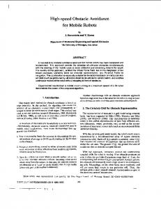
Fig. 4: Upper-left corner: left image. Upper-right corner: right image, destination point of view. Lower-right corner: left image homography-warped to the destination point of view. Lower-left corner: Absolute value of the right image minus the wapred image. Windows that do not pass the first test (as the one in red) are verified through a cross-correlation test (image patches in blue).

only difference is that we resize the input image for the first stage to reduce the computational cost. Thus, each output pixel represents a window in the actual input image. Those windows classified as obstacle by the first stage are then verified or discarded by the second one. The aim of the second stage is to filter false positives. In order to do this, it is tried to find a match for the image patches of the destination point of view image corresponding to windows classified as obstacle by the first stage within a double-sized window in their correspondant position in the warped image. The match is only searched within a slightly bigger window in the same position because the image is already warped (under ideal conditions there would be a perfect match for every floor-window in exactly the same position). It is outlined in figure 4. This comparison is carried out by computing maximum output for cross-correlation. If the maximum for any of the channels is under a threshold, the window does not pass the test and it is classified as obstacle. Color information allows us to differentiate between different colors that have the same luminance. Here, a relatively low threshold should be used. The key idea is that it is safer and more stable to decide based on multiple low thresholds of different nature that complement each other, than using a single highly tuned one. Since only candidate windows are tested, this second stage improves significantly the classification process without adding too much computational overload. This improvement not only decreases the occurrences of false positives on edges of textured floors, which is the biggest disadvantage of similar techniques, it also allows to dismiss low objects that do not actually represent an obstacle for the robot. In any case, no matter how approximate they are, there will be two different

5

homographies, the actual homography that the floor induces in the two cameras, and the homography we are estimating. The second step allows these two homographies to be reasonably different without compromising the system. Unlike shadows, which do not depend on the location of the observer, light reflections do. While shadows are just low illuminated areas, light reflections are a different phenomenon in which the floor acts as a mirror. Thus, light sources are imaged on different positions depending on the point of view of the camera, just like any object reflected in a mirror would. Unfortunately, this highly common phenomenon makes reflected light sources appear on a non-floor altitude. Even though they might not be detected and identified as proper reflections, and despite they can ruin the geometric classification we can still deal with them due to: • robots do not actually walk over mirrors, reflections are diffuse • the use of polarizing filters reduce reflections • the second test reduces the impact of the remaining reflections The main improvement of this algorithm to previous approaches is that it is partially immune to inaccurate homographies. Little variations on the actual homography produce mostly a translation of the image and little projective deformation. For every window passing the first test, the best correlation match is searched in its neighbourhood. If a window is not an actual obstacle it should have a good correlation match and should be discarded by the second test. As outlined before, this problem is very common when using mobile robotic heads. The scenarios in which this might be helpful are: • Loose or wrong camera position estimation: Small translations or rotations of the robotic head, due to looseness or small impacts, may change the actual homography. In such cases, other approaches would give lots of false positives. • Motorized stereo configurations: When the homography is recalculated in real-time in a stereo system, wrong pose and angle estimations, due to the imperfections of hardware or software, may lead to inaccurate homographies. This would also lead to false positives if using other approaches. • Camera desynchronization: Even slight camera desynchronizations often make previous algorithms useless. This might or might not be common depending on the hardware used. Once the second test is finished a binary image where pixels represent small windows of the original images is obtained. Assuming that the destination point of view is the one of the right camera, the process can be summarized as follows: 1) Copy the right image, I R , to a temporal image I T 1 . 2) Use H to warp the left image, I L , to I T 1 . 3) Compute the absolute value of I T 1 - I R . Store the result in I T 2 . 4) For each window having a pixel over a threshold: a) If the maximum value for the normalized crosscorrelation value in a bigger window is over a

6

JOURNAL OF PHYSICAL AGENTS, VOL. 4, NO. 1, JANUARY 2010

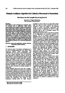
threshold for all channels, set the window as floor. b) Else set the window as obstacle. The first step can be skipped if, after the algorithm is finished, pixels outside binocular space are ignored. Optionally, if a window size resolution is not enough, a flood-fill operation can be started on the windows that passed the second test after resizing the output image. III. C OLOR - BASED DETECTION The color-based obstacle detection is inspired on the approach seen in [5], pixels are classified based on their presence in a histogram which is obtained after a training process. The training consists in the selection of several image regions of the ground and the computation of a three dimensional histogram from those image regions. Region selection can be done manually by a human operator or, if the environment obstacles are textured (e.g. there are no untextured walls), by the robot itself selecting floor regions using the geometricbased classification previously detailed. Instead of using two separate 1-dimensional histograms as suggested in [5], we use a single 3-dimensional one. The use of a three dimensional histogram is justified in terms of discrimination power. A 3-dimensional histogram is more powerful than a 1-dimensional one (i.e. a 3-dimensional histogram will always have, at least, the same information as a 1-dimensional one) and it is in no means harder to use. Even several threshold cuts on different 1-dimensional histograms will always sum up to axis paralell decision boundaries on corresponding multidimensional histograms. Despite the size of the histogram goes from n to n3 , by using 3-dimensional histograms we dramatically improve the color classification, without considerable time implications. Figures 5a and 5b show the difference of distriminative power graphically. We build our 3-dimensional histogram with values for normalized red and green components and an approximated value of luminance. Depending on the number of bins in which an axis is divided, we will get a different invariance for the values stored on it. The more bins an axis has the less invariance it gets. In particular, luminance invariance is desirable to some extent, but a complete invariance would entail a loss of discriminative power. A reasonable way to build the histogram is to divide the X and Y axis in 128 bins and 32 bins on the Z axis. Thus, assuming that pixels are represented as RGB bytes (so their values range from 0 to 255), the X, Y and Z axis values would correspond to: 128R/(R + G + B + 1)

(3a)

Y : 128G/(R + G + B + 1) Z: (R + G + B)/12

(3b) (3c)

X:

Once the histogram is generated, it is low-filtered using a 3x3x3 mask and the training is finished. Despite most color based obstacle detectors use HSV color space, we decided not to use it because hue values are usually very noisy at low saturation or low luminance. While other approaches as [5], [6] do not take into account pixels with low saturation, experimental results proved that greyish

(a) Discriminative power of a 2-dimensional histogram.

(b) Discriminative power of two 1-dimensional histograms.

Fig. 5: Comparison between the discriminative power of a 2-dimensional histogram and two 1-dimensional histograms. This can be extended to a third dimension. The striped area of figure delimits the boundary of two 1-dimensional histogram while the grey area delimits the frontier of the 2-dimensional histogram.

pixels should not be ignored. Obviously, the floor or some of the obstacles may be gray. Our three dimensional approach histogram shows better performance in the experiments. In [15] a similar approach is taken, but it uses a two dimensional histogram, with normalized red and green values only. Thus, it is fully luminance invariant, which, as previously seen, is rarely a desired feature. As well as in the geometric cue, the classification is divided in two stages. In the first stage, each pixel is classified according to the presence of its color in the histogram. If the quantity is lower than a threshold, the pixel is classified as obstacle. This threshold can be set as a percentage of the histogram population so it does not depend on the size of the training set. In the second step of the color-based classification the output is windowized by taking only the pixel with the

MANSO ET AL.: OBSTACLE DETECTION ON HETEROGENEOUS SURFACES USING COLOR AND GEOMETRIC CUES

lower value for each window. For this purpose 4-pixel width windows are used (i.e. a 4x4 window is classified as obstacle only if every pixel of the window have been classified as obstacles). This step removes false positive produced by noise. IV. M ULTIPLE CUE OBSTACLE DETECTION An obstacle detection system based on only one of the described methods would perform well under certain circumstances: planar floor and textured obstacles in the geometric approach; and disjoint color sets for obstacles and floor in the color-based one. Since these conditions are seldom found, the quality of such classifications can be improved by using both at the same time, taking advantage of the different properties of the cues. A color-based only classification would often lead to non desirable classifications such as classifying as obstacle a paper sheet lying on the floor. On the other hand, a geometric-based only classification would not see any obstacle in an untextured wall. We suggest using both cues in order to produce a higher-quality classification. Nevertheless, we also claim that merging the results of both classifiers should be carried in a more sophisticated way than AND/OR operators. Both, planar perspective mapping and color based cues are merged in order to get a single binary image as output, where each pixel is related to one of the windows of the single cue classifiers. As we will see in section V, the fusion of cues of different nature allows the robot to navigate through unstructured as well as structured environments. The only restriction is that the ground must be locally planar. The cue fusion process is ruled by the two following principles: 1) Geometry wins on small obstacles: Here the main assumption is that a region classified as obstacle by its color, that is not classified by the geometry-based obstacle detector, is probably a planar object lying in the floor (or part of it) which does not actually represent an obstacle for the robot. Thus, unless the second principle tells the opposite, they should not be classified as obstacle. According to this, isolated regions classified as obstacles by their color, and not by the geometry-based obstacle detector, are ignored. 2) Color wins on large tall obstacles: In indoors environments walls are very common. Since usually they are untextured, the planar perspective mapping approach might not classify them correctly. Big regions reaching the horizon line are suspicious enough to assume they are untextured walls (or any other obstacle). This kind of regions are classified as obstacles despite they are not detected by the geometry-based algorithm. Thus, the whole connected area is classified as obstacle. Following this two principles the visual field of the robot is divided in two areas, the one under the horizon line and the one above it. In the lower zone the geometric cue prevails, while in the upper one it is the opposite. In case that the connectedarea of a region classified as obstacle by its color comprise part of both zones, the whole connected area is classified as obstacle. This particular aspect can be seen in figure 6. It is reasonable to think that there is no point classifying by their color the image zone above the horizon line because it is

7

already known that its pixels correspond to obtacles assuming a planar floor. Nevertheless, because connected-areas may span part of both zones, the method provides new information. This is specially important in order to avoid walls or dodge tall untextured obstacles.

Fig. 6: This picture shows the horizon line (in red) and the connected-areas classified by their color that span part of the under-horizon area (dashed). The horizon line of a plane can be calculated as the image line going through two different vanishing points of lines belonging to the same plane. According to [1], the vanishing point of a line is the intersection of a parallel line passing through the camera center with the image plane. In [1] it is demonstrated that under a projective camera P = [K|I] the vanishing point v of a line is imaged as: v = Kd

(4)

being d a bound vector representing the direction of the line. As can be deduced, for a particular camera, the vanishing poing of a line only depends on its direction. Thus, in order to get two different vanishing points of lines belonging a particular plane, it is necessary to use intersecting lines. Given a vector n0 normal to the plane of interest π (usually (0, 1, 0)) and a camera K whose extrinsic parameters are known, such directions can be easily calculated. The extrinsics parameters are needed to transform n0 to the frame of reference of the camera, hereafter n. Thus, the two directions can be computed as: d1(x) = +2000

(5a)

d2(x) = −2000 d1(z) = 10000

(5b) (5c)

d2(z) = 10000

(5d)

d1(y) = d1(z)n(z)/n(y) + d1(x)n(x)/n(y)

(5e)

d2(y) = d2(z)n(z)/n(y) + d2(x)n(x)/n(y)

(5f)

V. E XPERIMENTAL RESULTS The described system leads to a binary image which can be easily used for navigation. The floor boundary can be calculated by scanning the columns of the binary image bottom-up,

8

JOURNAL OF PHYSICAL AGENTS, VOL. 4, NO. 1, JANUARY 2010

constructing a polyline with the first occurrences of obstacle pixels in the image. Also, if the extrinsic camera parameters are known, assuming that obstacle pixels are near the floor, the binary image can be mapped into world coordinates. With the binary image mapped to world coordinates, a laser measure can be estimated and thus, local navigation can be solved by using any of the existing range-based algorithms such as VFH+ or Potential Fields[11]. Figures 8, 9 and 10 are examples of the output of the obstacle detection system. The left obstacle of figure 8 and both obstacles of figure 10 are detected by both geometricbased and appearance-based algorithms. The wall at the right of figure 8, only has texture at its bottom, which actually lies on the floor plane, thus, it can only be detected by its appearance. The system is also able to discard the planar objects lying on the floor which appear on figures 9 and 10. In all of these figures floor plane is represented by light colored lines and obstacles are represented by dark ones. The rest of the section will introduce the robot platform used and the results of the experiments which lead us to the conclusions that follow in section VI. A. Description of the used robot platform The obstacle detection system has been tested on RobEx, a low-cost differential robot platform developed at the Robotics and Artificial Vision Laboratory of the University of Extremadura, previously used and described in[16]. The cameras are two USB webcams working at 20Hz. Both cameras are mounted on a three degrees of freedom head system. The computation is done on-board in real-time by a laptop carried by the robot. Even using a low cost robot and cheap cameras, the robot is able to navigate autonomously in real-time on a wide variety of environments. The robot is shown in figure 7.

polarized at some extent. We use this phenomenon to decrease the appearance of these reflections on the images by providing the cameras with circular polarizing filters, which remove polarized light (e.g. light reflections on the floor). Reflections are closer to full polarization as they approach the so called Brewster’s angle[14], which depends, in this case, on the refractive index of air and floor. Although light at angles far from the Brewster’s angle are only partially polarized and hence the polarizing filters do not remove the reflections completely, they have been proved to be helpful. B. Single vs. Multiple cue navigation Single cue navigation was performed on both structured and unstructured environments. The results obtained with the color based approach outperformed the ones obtained with previous similar methods, but it is still not reliable by itself. Ground surfaces and obstacles sometimes share the same color, specifically when the scene is highly or barely illuminated. Results obtained with the geometric approach clearly outperformed the ones obtained with previous similar methods. The overhead of the second test is negligible, as it is done only on candidate windows. In spite that the geometric obstacle detection is enough on unstructured environment where untextured image areas are very rare (with exception of the sky which is not an obstacle), on structured environments may be problematic.

Fig. 8: The obstacle and the wall are detected.

C. Sixty minutes challenge using multiple cues Fig. 7: RobEx is the robot we used in our experiments. As seen in section II, light reflections depend on the point of view of the camera, so they may lead to a wrong classification. Despite the impact of light reflections on the geometry algorithm is minimized using the second test, it may not be enough depending on the material of the floor. A useful property of electromagnetic waves, such as light, is that when they are reflected in a planar surface, they get

When the obstacle detection system development was started, a thirty minutes challenge was established as a measure of reliability. The challenge was passed in exceed when using cue fusion. In fact, it has passed several times a sixty minutes challenge. With geometric single-cue navigation, the challenge was also passed in unstructured environments (textured) but it failed in structured scenarios with untextured walls. On single cue navigation, the results depended heavily on the color of the ground and the obstacles. The scenario in which the sixty minutes tests have been succesfully accomplished is a specially tailored environment

MANSO ET AL.: OBSTACLE DETECTION ON HETEROGENEOUS SURFACES USING COLOR AND GEOMETRIC CUES

9

Fig. 9: Both, the paper sheet and the landmark, are discarded as obstacles.

Fig. 11: RobEx robot trajectory using a naive wandering algorithm. Fig. 10: Obstacles are detected, the paper sheet lying on the floor is discarded.

with tricky obstacles and non-obstacle objects with different heights, shapes and colors, as well as light reflections. A picture of this environment can be seen in figure 11, where the trajectory of a 7-minute wander is also shown. D. Real time homography estimation Due to the problems seen in II, specifically camera-camera desynchronization, camera-head position sensor desynchronization, and stereo head pose uncertainty, the approaches in [6], [15] are error prone when using motorized stereo heads. Because of the second test of the geometric classifier, our method discards false positives with reasonable desynchronizations or pose estimation errors. In our experiments, the real time homography estimation performed successfully even with rough camera calibrations. VI. C ONCLUSIONS In this paper we have presented two improvements to previous single cue detectors and a new technique for merging their outputs. The new single cue detectors, appearance and geometry based, outperform their previous counterparts. In addition, the proposed method for cue fusion clearly outperforms

any single cue detector, as well as the multiple-cue method detailed in [6]. Due to the variety of obstacles present in the tests, we have been able to demonstrate that our approach allows the robot to navigate through a wide repertoire of conditions. The computation is light enough to be carried in real-time on an average laptop, coexisting with other heavier software components. In order to improve significantly the system performance, our view is that it will be required a richer environment representation. The only situations in which the algorithm does not work as it would be desirable is when facing untextured obstacles with the same color as the ground (see picture 2) and with low height obstacles, no matter their color, with very little or no texture and a rounded shape (so that the obstacle is imaged in the same way as a planar object would). Generally these situations can be easily overcome with a dense, symbolic, geometric representation of the environment that can only be achieved using knowledge-based modelling techniques in conjunction with state-estimation algorithms. Steps are being taken towards this goal. ACKNOWLEDGMENT This work has been supported by grant PRI09A037 from the Ministry of Economy, Trade and Innovation of the Extremaduran Government.

10

JOURNAL OF PHYSICAL AGENTS, VOL. 4, NO. 1, JANUARY 2010

R EFERENCES [1] Richard Hartley and Andrew Zisserman, “Multiple View Geometry in Computer Vision”, Cambridge University Press, 2004. [2] J. Gaspar and J. Santos-Victor and J. Sentieiro, “Ground Plane Obstacle Detection with a Stereo Vision System”, in International Workshop on Intelligent Robotic Systems, 1994. [3] Jorge Lobo and Jorge Dias, “Ground Plane Detection using Visual and Inertial Data Fusion”, in International Conference on Electronics Circuits and Systems, IEEE, pp. 479-482, 1998. [4] Zhou and Baoxin Li, “Robust Ground Plane Detection with Normalized Homography in Monocular Sequences from a Robot Platform”, in International Conference on Image Processing, IEEE, pp. 3017-3020, 2006. [5] Iwan Ulrich and Illah Nourbakhsh, “Appearance-Based Obstacle Detection with Monocular Color Vision”, in ”in Proceedings of the AAAI National Conference on Artificial Intelligence, AAAI Press, pp. 886-871, 2000. [6] Parag Batavia and Sanjiv Singh, “Obstacle Detection Using Adaptive Color Segmentation and Color Stereo Homography”, in in International Conference on Robotics and Automation, IEEE, pp 705-710, 2001. [7] Y.I. Abdel-Aziz and H.M. Karara, “Direct Linear Transformation from Comparator Coordinates into Object Space Coordinates in Close-Range Photogrammetry”, in Proceedings of the Symposium on Close-Range Photogrammetry, American Society of Photogrammetry, pp. 1-18, 1971. [8] Wolfgang Boehler and Andreas Marbs, “Investigating Laser Scanner Accuracy”, Leica Geosystems HDS, 2003. [9] Jin Zhou and Baoxin Li, “Homography-Based Ground Detection for a

Mobile Robot Platform Using a Single Camera”, in in International Conference on Robotics and Automation, IEEE, pp. 4100-4105, 2006. [10] Thomas Bergener, Carsten Bruckhoff and Christian Igel, “Evolutionary Parameter Optimization for Visual Obstacle Detection”, in in The International Institute for Advanced Studies in Systems Research and Cybernetics, pp. 104-109, 2000. [11] Iwan Ulrich and Johann Borenstein, “VFH*: Local Obstacle Avoidance with Look-Ahead Verification”, in in International Conference on Robotics and Automation, IEEE, pp. 2505-2511, 2000. [12] Darius Burschka, Stephen Lee and Gregory Hager, “Stereo-based obstacle avoidance in indoor environments with active sensor re-calibration”, in International Conference on Rob otics and Automation, IEEE, pp. 20662072, 2003. [13] Scott Lenser and Manuela Veloso, “Visual Sonar: Fast Obstacle Avoidance Using Monocular Vision”, in International Conference on Intelligent Robots and Systems, IEEE, pp. 886-891, 2003. [14] A. Lakhtakia, “General Schema for the Brewster Conditions”, in Optik, Vol 90, pp. 184-186, 1992. [15] Yong Chao and Zhu Changan, “Obstacle Detection using Adaptive Color Segmentation and Planar Projection Stereopsis for Mobile Robots”, in International Conference on Robotics, Intelligent Systems and Signal Processing, IEEE, pp. 1097-1101, 2003. [16] Pilar Bachiller, Pablo Bustos and Luis J. Manso, “Attentional Selection for Action in Mobile Robots”, in Advances in Robotics, Automation and Control, I-Tech, pp. 111-136, 2008.