Multi-Feature Based Visual Saliency Detection in Surveillance Video Yubing Tong*a, Hubert Konika, Faouzi Alaya Cheikhb, Fahad Fazal Elahi Gurayab and Alain Tremeaua a Laboratoire Hubert Curien UMR 5516, Université Jean Monnet -Saint-Etienne, Université de Lyon, France, 42000 ; b Computer Science & Media Technology, Gjovik University College, PO BOX 191, Norway, N2802 ABSTRACT The perception of video is different from that of image because of the motion information in video. Motion objects lead to the difference between two neighboring frames which is usually focused on. By far, most papers have contributed to image saliency but seldom to video saliency. Based on scene understanding, a new video saliency detection model with multi-features is proposed in this paper. First, background is extracted based on binary tree searching, then main features in the foreground is analyzed using a multi-scale perception model. The perception model integrates faces as a high level feature, as a supplement to other low-level features such as color, intensity and orientation. Motion saliency map is calculated using the statistic of the motion vector field. Finally, multi-feature conspicuities are merged with different weights. Compared with the gaze map from subjective experiments, the output of the multi-feature based video saliency detection model is close to gaze map. Keywords: visual saliency detection, motion saliency, scene understanding, no camera movement
1. INTRODUCTION Under natural viewing conditions, humans tend to focus on specific parts of an image or a video naturally. These regions carry most useful information needed for our interpretation of the scenes. Itti’s attention model and GAFFE are two typical stationary image saliency analyzing methods adopting the ‘bottom-up’ visual attention mechanism1, 2. Image saliency map can be calculated by the image reconstructed by phase spectrum and inverse Fourier transform3. Phase only gives information on localization and orientation without intensity. So this may not be enough, other information of an image should also been considered. And video contains more information than a single image. The perception of video is also different from that of single image because of the additional temporal correlation. Through video displaying, we can obtain a clear and dynamic perception of the real scene with some factors such as who, where, what4. Papers have contributed more to the stationary image saliency map but seldom to video saliency map. Video saliency involves more information and is more complicated than image saliency5, 6, 7, and 8. The above saliency map methods are all based on the bottom-up model. Motion feature and other stationary features including color, orientation and intensity are viewed as low-level features in the bottom. Every feature is individually analyzed for feature conspicuity and finally combined for final saliency map. In fact, human perception is more complicated, both bottom-up and top-down framework should be involved. For example, just after looking at several frames in the start of a video, we might search the similar objects in the following successive frames unconsciously. And our eyes are able to catch those objects more easily, especially human faces. And for surveillance videos, the unconscious searching operation might be more distinct. After the several start frames, some scene information is confirmed, such as background information. Then foreground objects are detected and will be very probably focused on in the following frames. So in this paper, scene understanding is added into the saliency detection oriented surveillance *
[email protected]; phone 0033 04 77 91 57 51.
video. Based on the knowledge of scene including background generation and foreground extraction, we will have further perception of the video content including stationary and motion saliency map, and finally different saliency maps are merged with distance weights. The rest of this paper is organized as follows. In section 2, background generation and foreground extraction are introduced. Section 3 shows the stationary saliency map model, motion saliency map and the merging model based on them. Section 4 and section 5 contains the experimental results and discussions of future extensions.
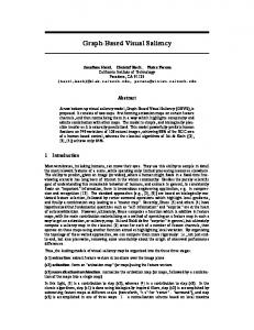
2. BACKGROUND GENERATION AND FOREGROUND EXTRACTION IN SURVEILLANCE VIDEO As for surveillance video, after background confirmation, our attention will be focused on the moving part in the foreground. So here background is firstly generated followed with foreground extraction. Background generation and foreground extraction are the basis for further saliency analysis in surveillance video. In a surveillance video without camera movement, the background is stable and only foreground objects emerge temporarily9. The current observed pixel depends on the effect of background, foreground and noise as shown in figure 1. li
hi Wi
(a) Same position pixel in different frames (b) Pixel intensity variation at the center of the dark circle Figure 1. Frames image in a station surveillance video.
A simple model for background and foreground is given as following,
Vobsv = Vbg + N noise + V fg
(1)
Where, Vobsv, the current observed pixel is consisted by background information Vbg, foreground information Vfg and noise Nnoise. In figure 1 (b), the noise makes the pixel value vary in a small range. Non-parameter background generation algorithms are focused on because of its simple theory foundation and low requirement on computation. We give a definition of background generation by using sliding window marked with red rectangle in figure 1 (b). For the sliding window Wi, there are five attributes with it: sliding window length (li), height (hi), mean value ( μi ), standard square error ( δ i ) and frequency number of the pixels emerging in this window (ni ). Background generation can be equal to find the best results of the following problem:
min
δi ni
,
⎧δ ≤ δ 0 with ⎨ i ⎩ni ≥ n0
Where, k is the current window number.
i = 1,..., k
δ 0 and n0 are constant value.
(2)
Since background is viewed to be stable and emerge often in video sequence, we think background part must emerge in the former part or the latter part in the video. A binary tree searching algorithm is used to find the best solution for equation (2) as shown in figure 2.
2N
2 N −i
2 N −i Figure 2. Binary tree searching.
2N frames in a surveillance video are chosen to generate background and they are divided into left part and right part as shown in figure 2. Each part will be further divided into two small left and right parts and for each part δ i and ni are calculated,
δi ni
from the left part and right part are compared. Then the smaller part will be chosen and divided again.
With such an iterative searching, a very small part which is just like a small window can be used to generate the background pixel. We can use the median value of this small window as background pixel value. So here our searching window moves in a ‘jumping’ mode instead of only sliding step by step with the increase of frame number10. In the above searching, every pixel will be detected which might involves many redundant calculation. Some background pixels might be estimated with several key frames for saving calculation, for example, the pixels in top-left corner in figure 3 are always stable in the whole video sequence, so pixel in this part might be viewed as background without further searching. Figure 3 shows the results of background generation is shown in figure 3 and the right bottom is the generated background image.
Figure 3. Generated background
Figure 4. Foreground extraction.
Foreground can be extracted by comparing the generated background and the current frame. Figure 4 shows some results of foreground extraction. We can see that the objects in foreground are extracted except for only a few points in those objects such as the part in the blue circle. With some other information, such as motion vector in the same object or in the same macro block, this case could be improved. If all the motion vectors in the neighborhood of the current block exist as shown in figure 5 (a), then the region in the extracted foreground should be continual. With motion vector field information, the blue circle in the above figure 4 could be improved as figure 5 (b).
(a) #173 motion vector (b) improved foreground Figure 5. Improved foreground extraction.
3. VISUAL SALIENCY MAP IN SURVEILLANCE VIDEO 3.1 Multi-feature stationary saliency map Low level features such as intensity, color and orientation contribute much to our attention in Itti’s bottom-up attention framework. Every feature is analyzed using Gaussian pyramid and multi-scales. 7 feature maps are generated including one intensity, four orientations (at 0, 45, 90,135 degrees) and two color components (red/green and blue/yellow) conspicuous maps. After a normalization step, all those feature maps are summed to 3 conspicuous maps: intensity conspicuous map Ci, color conspicuous map Cc and orientation conspicuous map Co. One drawback of Itti’s visual attention mechanism model is that its saliency map model is not well adapted for faces images. Psychological tests have also proved that face, head or hands can be perceived prior to any other details11. Several studies in face recognition have shown that skin hue features could be used to extract the face information. To detect heads and hands in images, we have used the face recognition and location algorithm used by Walther12. Then stationary saliency based on multi-features conspicuities can be described as,
S S = f ( S Itti , S Face )
(3)
1 (2Ci + 2Cc + Co + 3CF ) 8
(4)
An experimental adding weights model is given as,
SS =
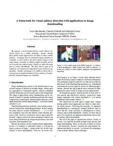
Figure 6 (b) showed the saliency map from the multi-feature stationary model and figure (c) showed the saliency map from Itti’s model. The result from the mixed model seems more reliable. Reference I18 of TID2008
50 100
height
150 200 250 300 350 50
100
150
200
250 300 width
350
400
450
500
(a) the original image (b) stationary saliency map (c) Itti map Figure 6. Saliency region from Itti’s model and our stationary model.
3.2 Motion saliency map With motion perception, we could know what is happening in the current scene. And some regions or objects are not so salient in video although they might be salient in images, for example, the rich texture of the object in images will be omitted in videos with fast motion. In this paper, motion information of a video is analyzed with its motion vector field which can be calculated using motion estimation with more than one reference image. Here we used full searching and block matching to find the best motion vectors which are normally used in video compressing. Based on the motion vector field, the intensity of motion vector, spatial coherence and temporal coherence of the motion are used to describe motion saliency map8. The intensity of motion vector is computed with the following equation,
I=
(mvx )2 + (mvy) 2
(5)
where, mvx is the motion vector in x direction (horizontal direction), mxy is the motion vector in y direction (vertical direction). Besides the intensity, the phase θ of motion vector will be also analyzed.
θ = arctan( θ
mvy ) mvx
(6)
distributes in [0, 360] after normalization.
ρi
Within the motion vector field, motion vector of the blocks will also be analyzed. The distribution probability density is computed using the histogram distribution of
θ
value within the neighbourhood with size of k x k, here 7x7 is used.
ρi =
Fnum _ i l
∑F i =1
(7)
num _ i
where, Fnum_i is the frequency number in ith bin of phase histogram. Figure 7 shows an example of the motion vectors in neighborhood and its corresponding phase values histogram distribution as following,
(a) Motion vector field in 7th frame (b) Histogram of the neighborhood of 145th MB Figure 7. Motion vector field and phase value histogram, in figure (a), the central blue rectangle means the current MB and the red rectangle means neighborhood, here 9 bins for histogram.
The spatial motion saliency Cs is calculated as following, N
C s = −∑ ρ i ⋅ lg ρ i
(8)
i =1
N is the number of histogram bins of
θ
value in kxk field.
Temporal saliency map Ct can be defined in the same way. Then motion saliency map is computed in the following equation
S M = I ⋅ Ct (1 − I ⋅ Cs )
(9)
I is motion intensity by computing the magnitude of motion vector, Ct is the temporal coherence inductor and Cs is the spatial coherency based on spatial phase histogram and temporal phase histogram statistic and analysis. 3.3 Merging model of stationary saliency and motion saliency The stationary saliency map SS and motion saliency map SM can be merged to obtain the final saliency map of every frame in a video. Since we usually more easily focus on those objects emerging into the center of observing window than that is far away from the center (xc, yc), we propose a distance weight fusing model as following,
SV _ G = α ⋅ S M ⋅ wi _ mb + (1 − α ) ⋅ S s
(10)
wi _ mb = e− d / 8
(xi − xc )2 + ( yi − yc )2
(12)
width _ mb height _ mb ; yc = 2 2
(13)
d= xc =
(11)
Where width_mb and height_mb are the height and width in mb (16x16),
wi _ mb is the block distance weight in 2D
Gaussian distribution. Beside the above fusing method, some other fuse mode are also designed for comparison including Mean, Max and pixel multiplication fusion mode as following,
SV _ mean ( x, y, k ) =
(S M
+ SS ) 2
(14)
SV _ max ( x, y, k ) = Max( S M , S S )
(15)
SV _ multip ( x, y, k ) = S M × S S
(16)
4. EXPERIMENTS AND RESULTS In this section, several surveillance video sequences recorded by ourselves are used in the subjective experiments and our visual perception model. The target of video saliency detection is to make the video saliency map from our model mimic the gaze map derived from subjective experiments. Eye movements of 20 subjects, aged between 25 and 42, have been recorded by a 50 Hz infra-red based SMI eye tracker. The subjects were shown surveillance videos on a 17 inch CRT display of resolution 1024x768 pixels under normal viewing conditions. A psychophysical experiment is performed to detect subject’s dominant eye. The distance maintained between the monitor and the observer is 60-70cm. The subjects were asked to just watch the videos as they normally do. Then subjects’ dominant eye has been tracked and tracked data has been saved on another system running SMI IView software. Gaze maps are constructed using acquired Eye tracks. First of all a frequency map is developed for each frame of each video by adding up all the eye positions of each subject. To mimic the Human Visual system the frequency map is then filtered by a Gaussian filter. It is important to find a suitable standard deviation σ for the Gaussian filter. These frequency maps are filtered by Gaussian filter of σ = 37 which was chosen to approximate the fovea in the gaze map, and all eye fixations were taken into account13. The size of the Gaussian window is 40x40 pixels. These Gaussian maps are then normalized and added to the original frame with the colormap variation of 64, where blue color shows the minimum value and red shows the highest or most salient region of the video frame. Figure 8 shows the SMI device and corresponding gaze map.
(a)SMI device
(b) the original image
(c) Gaze map for video frame 65 (d) mixed image Figure 8. gaze map derived from SMI device.
Where, figure (a) SMI infra-red eye tracker, (b) Eye-movements recorded data (d) Gaze map for video frame 65 (d) Gaze map with colormap added with original frame. Figure 9 shows two frame images in surveillance video and the corresponding mixed images with gaze maps and saliency map, figure (a) and (d) are two original frames in video; (b) and (e) are the mixed map of gaze map and the original image; (c) and (f) are two mixed image with saliency map superimposed over the original image.
(a)Original image
(b) Gaze map
(c) saliency map
(d) Original image (e) Gaze map (f) saliency map Figure 9. Frame image gaze map and saliency map.
Figure 10 shows the saliency map from different saliency models. Here some stationary saliency models such as Itti’s model [1], frequency tune saliency detection [15] and phase spectrum saliency model [3] are used for comparison. Frequency tuned model and phase spectrum model even give out texture in the background such as window curtain. But some salient regions in stationary frame image will not be salient when the video is being displayed. Compared with the results from saliency models and the subjective gaze map, our proposed saliency model is more close to subjective gaze map.
(a) The original image #21
(b) Gaze map image
(c) Saliency map image
(d) Gaze map
(e) Itti’s model
(f) Frequency tuned model (g) Phase spectrum model Figure 10. Comparison among different saliency models.
(h) Our proposed model
Besides subjective comparison, here NSS (Normalized Scanpath Saliency) is used to estimate the relationship between gaze map and saliency map as that in [7, 14]. For example, NSS can be used to compare gaze map and saliency map with the following equation,
NSS (k ) =
GV ( x, y, k ) × SV _ m ( x, y, k ) − SV _ m ( x, y, k )
(17)
δS
V _ m ( x, y ,k )
Where, GV ( x, y , k ) is human eye gaze map normalized to obtain unit mean, and from detection model.
δS
SV _ m ( x, y, k ) is the saliency map
is the standard square error. Another randomized eye movement gaze map is also
V _ m ( x , y ,k )
used introduced for saliency map comparison besides human subjective eye gaze map. The randomized gaze map means to associate to a frame of the current video the eye movement of subjects when they were looking at another video clip. If our model can predict the eye movement well, NSS of real gaze map and saliency map should be high and NSS of randomized gaze map and saliency map should be low. Table 1 gives out some data about NSS with real eye gaze map or randomized eye gaze map. Here we considered four saliency map derived from different weights fusing methods for stationary saliency map and motion saliency map. The results from the merging stationary and motion saliency model with Gaussian distance are best. Table 1. Gaze map and saliency map comparison.
Fuse mode Criteria
SV_mean
SV_max
SV_multip
SV_G
NSS on real gaze map
0.367
0.312
0.150
1.066
NSS on randomized gaze map
0.020
0.032
-0.15
0.195
1
We also compare our result with other saliency detection algorithm including itti’s model , frequency tune saliency detection15 and phase spectrum saliency3 as shown in table 2. Table 2. Comparison among saliency models.
Model criteria
IT
FT(Frequency Tune)
Phase Spectrum
Proposed
NSS on real gaze map
0.123
0.160
0.002
1.066
NSS on rand gaze map
0.136
0.189
-0.044
0.195
According to the above data, our method with NSS on real gaze map is much higher than other saliency detection models with the similar NSS value on random gaze map. According to the definition of NSS on rand gaze map, the randomized gaze map just used the gaze map of previous video sequence instead of random array generated by random functions. The results from our proposed model are more close to real gaze map of surveillance videos.
5. CONCLUSION
In this paper, a new visual saliency detection algorithm oriented surveillance video is proposed. With the knowledge of scene understanding in surveillance video, background generation and foreground objects extraction are analyzed, and then multi-features including high level feature such as face and other low level feature including color, orientation and intensity have been used to construct stationary feature conspicuity. Motion saliency map is based on the motion vector analysis and motion saliency map and stationary saliency map are merged. Compared saliency map with the gaze map of surveillance videos from subjective experiments, the output of the proposed model is close to gaze map. Here the model is effective for surveillance video without camera movement. Next more natural videos with camera movement will be involved since background analysis will be also more complicated in some background moving scenes.
REFERENCES [1]L.Itti, C.Koch and E.Niebur, “A model of saliency-based visual attention for rapid scene analysis” IEEE Trans. PAMI., vol. 20, No.11, pp.1254-1259, Nov. 1998. [2] Rajashekar, U.; van der Linde, I.; Bovik, A.C.; Cormack, L.K, "GAFFE: A gaze-attentive fixation finding engine," IEEE Trans Image Processing, vol. 17, No.4, pp. 564-573.2008. [3] Qi Ma and Liming Zhang. "Saliency-Based Image Quality Assessment Criterion", ICIC 2008, LNCS 5226, pp. 1124–1133, 2008. [4] L.-J. Li and L. Fei-Fei. “What, where and who? Classifying event by scene and object recognition”. IEEE Intern. Conf. in Computer Vision (ICCV). 2007. [5] Shan Li, Lee, M.C. “Fast Visual Tracking using Motion Saliency in Video”, ICASSP. vol.1, pp.1073-1076, 2007. [6] Brian Michacel Scacellat. “Theory of Mind for a Humanoid Robot”, Autonomous Robert, vol. 12, No.1, pp.13-24, 2002. [7] S.Marat, T.Ho Phuoc. “Spatio-temporal saliency model to predict eye movements in video free viewing”, 16th European Signal Processing Conference EUSIPCO-2008, Lausanne: Suisse, 2008. http://hal.archives-ouvertes.fr/docs/00/28/89/66/PDF/2008_eusipco_marat.pdf. [8] Yufei Ma, Hongjing Zhang. A model of motion attention for video skimming. Vol.1, pp.22-25, ICIP 2002. [9] Desihe Sidide, Oliver Strauss, W.Puech "Automatic background generation from a sequence of image based on robust mode estimation", SPIE-IS&T Electronic Imaging, Digital Photography. 2009. http://hal-ujm.ccsd.cnrs.fr/docs/00/35/72/28/PDF/sidibe_spie2009.pdf. [10] Hanzi Wang, David Suter. “A novel robust statistical method for background initialization and visual surveillance”, ACCV 2006, LNCS 3851, pp.328-337, 2006. [11] R Desimone, TD Albright, CG Gross and C Bruce. "Stimulus selective properties of inferior temporal neurons in the macaque", Journal of Neuroscience, vol.4 pp.2051-2062, 1984. [12] Walther, D., Koch, "Modelling Attention to Salient Proto-objects", Neural Networks 19, 1395–1407, 2006. [13] Jost, T., Ouerhani, N., von Wartburg, R., Müri, R., and Hügli, H. 2005. “Assessing the contribution of color in visual attention”. Compute. Vis. Image Underst. Vol.100, No.1, pp.107-123, 2005. [14] S.Marat, T.Ho Phuoc, L.Granjon, N.Guyader. “Modelling spatio-temporal saliency to predict gaze direction for short videos”. International Journal of Computer Vision, vol.82, No.3, pp.231-243, 2009. [15] Radhakrishna Achanta, Sheila Hemami and Francisco Estrada. “Frequency-tuned saliency detection model”, CVPR2009. http://ivrgwww.epfl.ch/supplementary_material/RK_CVPR09/index.html.