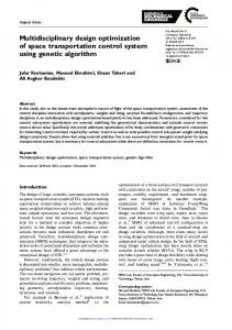
disciplinary design optimization of regional and business jets. ... to the optimization of a large business jet comprising winglets, rear-mounted engines and .... a variety of optimization and search methods, and can also be trained to use the ...
Multi-Fidelity Multidisciplinary Design Optimization of Metallic and Composite Regional and Business Jets Antoine DeBlois∗ and Mohammed Abdo† Bombardier Aerospace, Montreal, Qc, H4S 1Y9, Canada
This paper presents an aircraft manufacturer’s methodology for the high-fidelity multidisciplinary design optimization of regional and business jets. The formulation of the multiobjective function and the hybrid multi-level optimization architecture are highlighted. The high-speed aerodynamics sub-space is analyzed with a Transonic Small Disturbance code whereas the low-speed sub-space is analyzed using a three-dimensional panel code and the Valarezo criteria. In addition, the multiple design load cases including manoeuvre and landing are presented along with the fluid to structure load transfer scheme. Particular emphasis is also placed on the development, the industrial sizing and the structural suboptimization of a high-fidelity 3D FEM for composite and metallic wing structures. The validation of the structural sizing methodology is highlighted through examples and by comparison with typical aircraft wing structures. The influence of low-speed aerodynamics on the final design is emphasized and a comparative study between the multidisciplinary optimization of composite and metallic wings is presented. The methodology is applied to the optimization of a large business jet comprising winglets, rear-mounted engines and a T-tail configuration. The aircraft-level design optimization goal in this instance is to minimize a cost function for a fixed range mission assuming a constant Maximum Take-Off Weight.
Nomenclature CFD CSM PSE OBJ M T OW M LW ZF W Wres AW SOM ∆CpT E Va Vs Vv Rmax δv Subscript c c ∗ Engineering † Engineering
Computational Fluid Dynamics Computational Structural Mechanics Principal Structural Elements Top-level objective function Maximum Take-Off Weight, lbs Maximum Landing Weight, lbs Zero-Fuel Weight, lbs Reserve Fuel Weight, lbs Automatic Wing Structural Optimization Module Pressure delta between peak and trailing edge Maximum maneuvering speed, kts Stall speed, kts Vertical speed of descent at landing, kts Maximum ground reaction at landing Shock strut stroke, in
f F GA Λ AR TR ∆mass Nz α, �, kM Md Mc Mmo x y z
Cruise or Compression (Structures section) Tension
Professional, MDO lead, M.Eng., MCASI, MAIAA. Specialist, M.Eng., PhD, MBA, MCASI, SMAIAA.
1 of 25 American Institute of Aeronautics and Astronautics
stress, psi Allowable, psi Genetic Algorithm Leading Edge Sweep Aspect Ratio Taper Ratio Weight delta w.r.t reference Load factor Empirical regression coefficients Mach Dive Mach cruise Maximum Operating Mach Chordwise coordinate Vertical coordinate Spanwise coordinate
I.
Introduction
ultidisciplinary Design Optimization (MDO) is a mandatory enabler in obtaining efficient designs M that respect all aspects of the mission requirements. The concept of MDO has been implemented throughout many industries, particularly for the aircraft manufacturers, for which disciplines strongly conflict 1
each other. Nevertheless, the implementation of MDO remains a challenge due to the associated computational cost and the organizational complexity. A well-defined framework is necessary to perform an optimization process using simulation models of enough fidelity and complexity, in the specified time. The models must be accurate enough to properly capture the proper sensitivities to both the small and large changes that occur during the optimization process. To obtain such accurate predictions, high-fidelity computations are required throughout the process: from the simulation models through to post-processing, including the exchange of information between disciplines.2–5 The present paper aims at presenting a practical and computationally feasible methodology for composite and metallic multidisciplinary sizing and optimization from an aircraft manufacturer perspective. A review of a methodology to minimize the complexity of the design space by decomposing the optimization problem into smaller more tractable problems is also presented. Because of their potential weight saving, composite materials have received a great interest in the aircraft industry.6 Due to intense analytical and experimental work, aircraft manufacturers have built a high level of confidence in composite structural design procedures. Composites are no longer confined in secondary structures such as fairings; they constitute the major part of the primary structure. Therefore, a comprehensive MDO framework should include both metallic and composite materials. This will provide a proper optimization environment for accurate assessment and comparison between metallic and composite aircrafts. The structural properties of the wingbox will be assessed by an in-house automatic structural sizing tool that uses 3D Finite Element Model (AWSOM7 ). In addition, aerodynamicists usually perform manual iterations to alter the high-speed (transonic) optimized design to meet low-speed requirements. Such procedure is lengthy and the final design is not guaranteed to be a true optimum. This work presents how low-speed aerodynamics can be introduced in the MDO architecture, and how it impacts the final wing design. The interactions between the coupled design variables within this multi-disciplinary framework will be analyzed through a generic business jet optimization.
II.
MDO architecture
The high level of complexity of the design space of aircraft multi-disciplinary optimization is tributary to the high number of design variables and constraints; a proper architecture is required to mitigate the associated computational cost. As explained by Tedford and Martins,8 the multiple disciplines can be integrated using either single-level or multilevel formulations. On one hand, single-level approach (integrated approach) considers a single optimization problem, perturbing the entire set of design variables. At each iteration, the multidisciplinary state is converged by solving the coupled system. Typical integrated approaches include Multidisciplinary Design Feasible (MDF)9, 10 and Individual Design Feasible (IDF).9, 10 On the other hand, multilevel formulation employs embedded disciplinary optimization processes that perturb only a local set of design variables. The latter formulation decreases the computational complexity of the top-level optimization process. Typical bi-level formulation include notably Collaborative Optimization (CO).11 As demonstrated in Tedford and Martins work (Ref. 8), CO performs well on problems for which the number of local design variables is much larger than the number of coupling variables. The optimization architecture proposed in this work is a hybrid formulation between MDF and CO, similar to the asymmetric formulation developed by Chittick.12 A top-level non-linear gradient based optimizer controls the global design variables and aims at minimizing the overall objective function, OBJ. The terminology hybrid is used to highlight the fact that there is a single sub-problem: a subspace optimization controls the structural (local) design variables, and aims at minimizing the structural mass. This subspace was introduced to address the high number of structural design variables and constraints. In the present case, these are two orders of magnitude higher than the coupling variables (the Aerodynamics loads and Structural displacements). Figure 1 depicts the overview of the multi-level multidisciplinary optimization framework. The essential components will be briefly described hereafter. The iterative computational procedure is integrated into the optimization framework of iSIGHT, a com-
2 of 25 American Institute of Aeronautics and Astronautics
Figure 1: Overview of the hybrid Multi-Disciplinary Optimization formulation
mercially available software developed by Dassault-SIMULIA. iSIGHT is used to optimize the top-level composite objective function and viability of the constraints by perturbing the global design variables. iSIGHT is also used to control the running of the various codes in sequence and in parallel. The software proposes a variety of optimization and search methods, and can also be trained to use the most suitable hybrid combination of various optimization algorithms for a given problem. II.A.
Composite Objective Function
The top-level optimizer’s objective is to minimize the weighted sum, OBJ of all the individual objective functions. X OBJ = (wi fi )/si (1) i=0
P where the wi are the weighting coefficients, si are scaling factors and wi = 1.0. The weighting coefficients are a measure of the relative importance of each objective function - their magnitude is determined by the mission requirements. The scaling factors are introduced to cater for the difference in the order of magnitude of the objective functions; their influence will be discussed in the present paper. There are two objectives in the current implementation: minimizing M T OW for a fixed range and maximizing CLmax ; CLmax is in the range of unity, whereas the fuel weight is in the range of thousands. The maximum take-off weight is the sum of the maximum zero-fuel weight, M ZF W and the fuel weight, Wf uel . The fuel weight and structural weight are combined into a composite objective function based on the derivation of an integrated range model and using the fractional change methodology.13 It is based on a series of prediction algorithms applicable for personal/micro turbofan aircraft, business aircraft from very light to ultra-long range categories to commercial aircraft from commuters to narrow-body transports 3 of 25 American Institute of Aeronautics and Astronautics
of around 100 passengers. The underlying assumption in this problem statement is that an initial sizing of the aircraft and power plant has been performed (a priori) to address the mission requirements defined for the aircraft, i.e. payload, range, balanced field length, initial climb altitude capability, etc. This initial sizing defines the basic aircraft layout, M T OW , thrust-to-weight ratio, and wing loading and reference area. An algebraic expression of a new prediction of the flight fuel (for a given iteration during the active MDO scheme) that equates the aerodynamics and structures trade-off explicitly is given by equation 2. Wf uel(new) =
f Wf uel(ref ) (∆Wstr + ZF Wref + Wres(new) ) M T OWref − f Wf uel(ref )
where (1 + /R)(1 + /ZF W )� f= (1 + /ηe )(1 + /(L/D)) �
(2)
�1/α (3)
and the fractional change of range /R, zero-fuel weight, /ZF W , and lift over drag ratio, /(L/D) are given by: Rtarget ZF Wnew (L/D)new /R = − 1, /ZF W = − 1, /(L/D) = −1 (4) Rref ZF Wref (L/D)ref and the overall powerplant efficiency, /ηe is given by: /ηe =
(1 + /M )(1 + τM ) Mtarget − 1, /M = −1 1 + τM (1 + /M ) Mref
(5)
The parameter τM = kM Mref and kM is derived empirically and is specific to the engine being modeled. A typical interval of values for transport aircraft with respect to mission dependent regression coefficients are α = 1.36 to 3.08, � = −1.14 to −0.36 and kM = 1.85. In addition, ∆Wstr is the change in structural empty weight from the reference Manufacturers Weight Empty, M W E0 and Wres(new) is the combined block maneuvering, hold and alternate reserve fuel quantity. For a typical flight mission, one can assume that the change in reserve fuel is small (i.e. Wres(new) = Wres(ref ) ). For a fixed range mission, the seed and reference ranges are equal and hence the range fractional change yields /R = 0.0. The composite objective function shown below, where the minus sign is introduce to cater for CLmax maximization. w1 ∆mass w2 CLmax OBJ = − (6) s1 s2 with ∆mass = Wf uel(new) − Wf uel(ref )
(7)
The parameters wi and si will be discussed in section VII.A.1. II.B.
MDO process
The global design variables pertain to the planform and the airfoil profiles (a methodology developed by reference 14, but modified internally). Once a global design variable is perturbed, the optimizer sends the information in parallel to both the high-speed and low-speed CFD modules to generate the cruise, design and low-speed (take-off and landing) pressures. An in-house developed Transonic Small Disturbance, TSD, code (KTRAN15 ) is used for the high-speed aerodynamics characteristics whereas a commercial panel code (VSAERO16 ) is employed for the low-speed analysis. Upon calculation of the pressure fields, the structural properties of the wing have to be computed through the structural subspace optimization process. The local structural design variables are optimized using an in-house developed code (AWSOM7 ). The latter generates a 3D high-fidelity Nastran Finite Element Model (FEM), then performs a fluid-to-structure load transfer and finally sizes the wing structure through minimization problems. AWSOM uses either an inhouse developed Genetic Algorithm optimizer based on NSGA-II methodology17 or an in-house developed gradient-based constrained optimizer based on Interior-Point Method,18 depending on the nature of the material choice (either metallic or composite). Once the skin-stringer panels, ribs, spars and spar caps are designed satisfying structural failure modes, the wing box structural model is then used to calculate wing flexural properties. The static aeroelastic convergence is obtained using a fixed-point method, in which external loading is refined by successively converging wing deformations. This refined wing loading yields a
4 of 25 American Institute of Aeronautics and Astronautics
more accurate estimate of the wing weight. To reduce computational time, the aeroelastic convergence of the low-speed case is not performed - the aerodynamic pressure field is rather obtained at the flight twist (hence the one-sided arrow from low-speed module to Structures module in Figure 1). To reduce the complexity of the computational space and thus increase the degree of success in achieving a global optimum, the global design variables are optimized in a decoupled fashion. The approach adopted was to decompose the wing optimization problem into two separate, sequential optimization problems. 1. In the first pass, the wing planform is optimized while the sectional profiles and spanwise loading are held constant. The optimization technique that is chosen for this step is a nonlinear trained optimizer that is suited for all types of design space topographies (linear, nonlinear and rough). 2. In the second pass, the wing sectional profiles are optimized. During this last optimization, the wing planform shape is held fixed. The profiles are optimized two at a time sequentially along the span. The optimization technique is a nonlinear gradient-based optimzer called POINTERTM developed by iSIGHT (formerly Synaps) for aircraft preliminary MDO. This two-pass process is repeated until the minimization of the complex objective function is sufficiently converged. Throughout this process, it is very important to keep the lift coefficient constant within a tight tolerance to preclude the tendency of the optimizer to increase the L/D by simply increasing the CL. The total lift coefficient is kept constant by modifying the angle of attack. Fuel volume is continuously monitored upon completion of a design iteration to ensure that the wing has enough room to contain the fuel required for the specified aircraft mission. Another key aspect of interest within an industrial optimization environment is the feasibility of the design. Constraints are introduced to preclude the optimizer from exploiting the loopholes of the setup. For example, the landing gear has predefined thicknesses at its attachment points and chordwise location have to be within predefined limits. The high-lift devices such as the flap have to fit within the volume. When a design is considered infeasible, it is unnecessary to perform the costly CFD calculations and thus the setup assigns an important penalty to the objective function. Finally, in an optimization context, the concept of robustness is also a key parameter. One example is that the setup has to cater for failed CFD runs. In a gradient-based environment, there is the paradox of assigning a penalty sufficient enough to prevent the optimizer from choosing this failed design, yet low enough so as to prevent the optimizer from diverging due to false gradient values. The following sections will describe each component of the optimization set-up in more details.
III.
Computational Aerodynamics Analysis
Due to the different nature of the physics throughout the segments of the mission, there are two CFD code used in the framework. At take-off and landing, the compressible effects are negligible and thus an incompressible panel code is sufficient to model the flow behaviour. At cruise or at 2.5g, there are important compressible effects and possible flow separation, which implies a compressible, viscous code (or viscous correction effects). Moreover, the F.A.R. definition of the balanced manoeuvre is ”assuming the airplane to be in equilibrium with zero pitching acceleration, (...)”19 (§25.331(b)). Therefore, the high-speed code has to have trimming capabilities. III.A.
High-Speed Aerodynamics
The key challenge of computational fluid dynamics is to generate accurate results, in a feasible amount of time, for increasingly complex simulations and underlying flow physics (flow separation, shock-wave, etc.). At Bombardier Aerospace, the CFD code KTRAN15 has been widely used for optimization. KTRAN solves a modified TSD equation using Cartesian grid embedding techniques, coupled to boundary layer calculations on the aircraft lifting surfaces. This code is particularly interesting for the present purposes since it has an embedded cartesian grid meshing capability and thus new geometries are easily re-meshed. It can be used to model full aircraft configurations in a modular fashion, including fuselage-mounted or wing-mounted nacelles, wing-tip winglets, and, vertical and horizontal tail components that can be either fuselage-mounted or in a T-tail configuration. Modelling the full aircraft allows trimming, thus simulation of steady symmetrical manoeuvres. 5 of 25 American Institute of Aeronautics and Astronautics
CL
Although the TSD approach is of low-fidelity formulation, it provides reliable predictions of wing 3% drag pressure distributions, drag and aerodynamic loads at aircraft design conditions, i.e. at conditions with relatively weak shock waves and attached flow. In cruise cases, the accuracy of the drag prediction is usually within 2-3% of flight test measurements.13 Figure 2 illustrates the KTRAN drag predictions compared to flight test data for a trimmed ChalChallenger 300 - KTRAN prediction - M=0.6, Re=13.6M lenger 300 aircraft. This accuracy is critical in the Challenger 300 - KTRAN prediction - M=0.8, Re=13.6M Challenger 300 - FLight Test - M=0.6, Re=13.6M optimization process since it directly influences the Challenger 300 - FLight Test - M=0.8, Re=13.6M accuracy of the objective function. CD However, at the extremities of the flight envelope where either strong shock waves or flow separation Figure 2: KTRAN drag prediction versus comparison are present, the accuracy of KTRAN diminishes and with flight test data for the Challenger 300 aircraft. the code can diverge. Mach dive, Md is determined by reference 19, §25.335(b), but is usually in the vicinity of maximum operating cruise Mach number, Mmo , plus a 0.07 margin (Mmo = Mc + 0.07). Since business aircrafts fly at a high cruise Mach number, Mach dive can be close to 1.0. At such free stream Mach number, there exist strong shock waves at the upper and lower surfaces close to the trailing edge. The robustness of KTRAN at high and low lift coefficients (2.5g and -1.0g) and for high Mach numbers shown to be acceptable. To achieve high levels of confidence and robustness in the CFD analysis, the maximum Mach number was limited to M ach = 0.90, even if it is below the Mach dive of the analysed configuration. To overcome this limitation, an Euler or Navier-Stokes solver needs to be used for the off-design flow conditions. Such extreme load cases are only used by the structural module for load application. Thus, the lack of accuracy in the pressure field at the extremities of flight envelope has a minor impact on the optimization process since the load case pressure field has an indirect influence effect on the objective function through the prediction of the wing structural mass. The critical parameters are rather the lift coefficient and the spanload. The lift coefficient ensures the proper amount of g’s are applied and the proper CFD ensures a valid applied bending moment. As the shock moves toward the trailing edge, the centre of pressure moves in the same direction and the applied torsional moment is changed. Therefore, at the proper lift coefficient, the effect of a cut-off Mach number is reflected in a lack of accuracy in torsional moment. III.B.
Low-Speed Aerodynamics
The low-speed characteristics have an explicit effect on the objective function though the maximum lift coefficient, CLmax . This prediction is obtained by a combination of a panel code and the Valarezo20 criteria. Based on the difference between the peak pressure and the trailing edge, ∆CpT E = |Cpmin − CpLE |, at each spanwise wing station, the Valarezo criteria can accurately predict CLmax as well as the stall spanwise location, ηcrit . The low-speed panel code that is used in the present analysis is VSAERO,16 which solves the irrotational and inviscid flows. VSAERO requires a surface panel mesh of the wing as well as its wake, which is usually generated manually. An automatic VSAERO mesh generator has been developed to generate an isolated, clean wing configuration mesh. For an isolated wing analysis, the cross-flow due to the interaction near the fuselage and the winglet effects are neglected. In addition, it is assumed that the low-speed characteristics of the clean wing configuration will influence the deployed configuration of the wing with flaps and slats. For a slatless configuration, this assumption is even more representative because the stall characteristics are mainly influenced by the leading edge design. Figure 3 shows the pressure distribution of the DLR-F621 isolated wing obtained using the automatic panel mesh generator and VSAERO. The right hand side of the figure shows the pressure field of the same case obtained by using Bombardier’s 3D Navier-Stokes code (FANSC22, 23 solver). The solution represents a M ach = 0.20, α = 8.0◦ attached flow case. As shown by Figure 4, the pressure coefficients and ∆CpT E are in very good agreement with the high-fidelity code, even near the fuselage. A small discrepancy at the trailing edge can be noticed. To obtain CLmax , the automatic mesh generator and VSAERO are run in sequence for a sweep of angles of attack, α. The trailing edge pressure differences are calculated at some stations along the span of the wing and are compared against the maximum difference prescribed by the Valarezo 6 of 25 American Institute of Aeronautics and Astronautics
Y X
Z
(a) VSAERO - isolated wing
(b) FANSC - wing-body
Figure 3: Pressure field (M ach = 0.20, α = 8.0) comparison on the DLR-F6 configuration
η = 0.216
-4.5
VALAREZO criteria DLR-F6 isolated wing CLmax = 1.7402 ηcrit = 0.7591
η = 0.433
-6
-4 -5 -3.5 -3
VSAERO FANSC
-4
-2.5 -3 -2
Cp
Cp
∆CpTE N-S
-1.5
α = 8.0 α = 10.0 α = 12.0 α = 14.0 α = 16.0 α = 18.0 VALAREZO
-25
-2
-1 -1 -0.5 0
0
∆CpTE VSAERO
1 1.5 -0.2
0
0.2
0.4
0.6
0.8
1
-20
1 2 -0.2
1.2
0
0.2
0.4
X/C
0.6
0.8
1
1.2
X/C
∆CpTE
0.5
-15
η = 0.650
-6 -5
-5 VSAERO FANSC
-4
VSAERO FANSC
-4
-10
-3
Cp
-3
Cp
η = 0.867
-6
-2
-2
-1
-1
0
0
1
1
2 -0.2
0
0.2
0.4
0.6
0.8
1
1.2
X/C
2 -0.2
ηcrit
-5
0
0.2
0.4
0.6
0.8
1
0.2
1.2
0.4
X/C
(a) Cp distribution comparison at α = 8.0
0.6
η
0.8
1
1.2
(b) ∆CpT E along the span for an α sweepVSAERO isolated wing
Figure 4: Low-speed characteristics (M ach = 0.20) comparison on the DLR-F6 wing-body configuration criteria. As shown in Figure 4, the present method predicts the stall of the DLR-F6 wing at CLmax = 1.7402 and at ηcrit = 0.7591. By using the automatic mesh generator and VSAERO, the computational time of a single VSAERO run is in the vicinity of 10 seconds on a single CPU for 30 spanwise x 100 chordwise panels mesh. The calculations time for a sweep of angles of attack from α = −4.0◦ to α = 20.0◦ with two degrees increment remains below 3 minutes, which is the approximate run time of the high-speed code (KTRAN). On the other hand, FANSC requires 94 minutes to converge (to 5 orders) the same case (single α run) by using 32 CPUs of an IBM P5-575 supercomputer on 9.5M mesh points.24 Thus, performing a Navier-Stokes alpha sweep is too computationally expensive and the added precision is not significant.
IV.
Computational Structural Mechanics
The structural simulation model must be of high-fidelity to predict accurate structural deformations and weight predictions. It must be geometrically representative of the Principal Structural Elements (PSE), which constitute the primary structure and carry the most part of the internal load. Moreover, the internal loads must be post-processed using accurate structural constraints, preferably the same used by the stress departments of aircraft manufacturers. Thus, 3D Finite Element Models (FEM) are needed early in the design cycle. A recent in-house Automatic Wing Structural Optimization Module, AWSOM, was developed to auto-
7 of 25 American Institute of Aeronautics and Astronautics
matically generate a representative wing structure given only the external lines of the aircraft, and compute its flexural and weight properties. To do so, the code first generates a NASTRAN 3D Finite Element Model that includes every PSE of the wing box (skin, stringers, spars and ribs), as well as all the structural elements on which the aerodynamic pressure is applied (leading edge, trailing edge and winglet). The code then performs a fluid to structure load transfer for all the load cases specified by the designer. Finally, AWSOM optimizes the structure using either a Genetic Algorithm (GA) or a gradient-based optimizer. The various modules of this program are described in the following sections. IV.A.
FEM Geometrical Representation
The parametrization allows great flexibility in terms of wing geometry (planform, airfoil profiles, etc.) and structural layout (ribs, spars locations and orientations, stringer height, etc.). The generated wing box structure is a semi-monocoque two spars configuration (skin-stringers). The same CAD files are used for both the aerodynamic solver and the automatic FE-mesher to ensure good geometric compatibility between structural and aerodynamic models. Figure 5 shows a typical structural configuration generated by the code. Apart from the missing manholes, the FEM is very similar to a certification model that is manually produced at Bombardier Aerospace.
Figure 5: Wing Principal Structural Elements (PSE) designed by AWSOM.
IV.A.1.
Boundary Conditions
The FEM boundary conditions are crucial to obtain the proper internal loads. The present paper considers a three points pinned wing to fuse connection. In addition, symmetry boundary conditions are applied at the symmetry plane: out-of-plane translation and the two out-of-plane rotations. Finally, a pin boundary condition is applied both at the front keel beam and aft keel beam. IV.B.
Load Transfer
The aerodynamic and structural solvers require different meshes, both in terms of size and topology. Aerodynamic grids require a much finer mesh in order to capture non-linear phenomena close to the boundary layer, whereas a relatively coarser structural mesh is sufficient to accurately represent the load path. The differences between the aerodynamic mesh and the structural mesh implies a load transfer from the aerodynamic solver output to the structural solver input. AWSOM uses the CFD pressure coefficients and applies them directly to the surface elements of the skins, as shown on figure 6. Using this technique, there is no need to generate shear, bending and torque curves; the lift coefficient, CL, and pitching moment, CM, are
8 of 25 American Institute of Aeronautics and Astronautics
matched implicitly. Since several independent load cases are applied, the interpolation of the pressure from the aerodynamic to the structural elements is performed in parallel.
Figure 6: A typical pressure distribution applied on an AWSOM FEM. The load cases (ailoads, inertia and landing) that are used to size the wing structure are described in the following sections. IV.B.1.
Aerodynamic load
The F.A.R. specifies in §25.331(b), ref 19, that the balanced manoeuvre must be investigated for the whole maneuverings envelope of the (V − n) diagram. That is to say that the aircraft must be sized for the worst combinations of load factor, speed, weight and altitude. To reduce computational time, the present paper addresses two manoeuvre cases, as shown in figure 7.
MACH Md Mc
ALTITUDE Altitude where Md is limited by compressibility effects Altitude where Mc is limited by compressibility effects
WEIGHT
N FACTOR
MTOW
2.5g
MTOW
-1.0g
Figure 7: Maneuvering conditions considered by AWSOM.
9 of 25 American Institute of Aeronautics and Astronautics
IV.B.2.
Landing loads
The structure is sized by a static landing case at sea level, 1.0g. The aircraft speed of this load case is the maximum maneuvering speed, Va . The latter is obtained from the information obtained by the low-speed nW analysis. Since CL = 0.5ρV 2 S , and the stall occurs at CLmax and n = 1.0g, the stall speed Vs becomes: s Vs =
2W ρSCLmax
(8)
The √ maximum maneuvering speed is extrapolated at n = 2.5g, along the same parabolic equation: Va = 2.5Vs . AWSOM can only handle clean wing configurations. Therefore, at take-off or landing, the applied torsion is not properly captured since the deployed high-lift devices move the centre of pressure aftward and thus increase the lever arm. The landing load conditions and assumptions are specified in ref 19, §25.473 The present methodology considers a limit descent velocity of Vv − 10f ps at the maximum landing weight, W = M LW . The lift equals the aircraft weight, hence n = 1.0g, as specified by §25.473(b). The magnitude of the concentrated point loads are calculated by balancing the kinetic energy and the landing gear deformation energy, as shown by equation 9 Ekinetic =Edef ormation Z δFv Vv2 W = Fv (δstrut + δtire )dδ 2g 0
(9)
where δFv is the strut stroke (the unknown) and Fv (δstrut +δtire ) is the force versus stroke and tire deformation curve given by the landing gear manufacturer. Once δmax is calculated, the maximum reaction at the ground, Rmax , is computed by equating the aircraft kinetic energy to the work done in the shock absorber: Rmax
Ekinetic = , ηstrut δFv
R δmax where ηstrut =
0
Fv (δstrut + δtire )dδ δmax Fv (δmax )
(10)
The parameter ηstrut is a measure of the shock strut efficiency as it is the ratio of the total dissipated deformation energy over the total stroke work. A typical oleo-pneumatic strut efficiency is in the vicinity of ηstrut = 0.80. The landing load cases consider that the aircraft touches the ground with both main landing gear simultaneously, hence Rmax corresponds to both the left and right main gears. The calculated main landing reaction is applied in the auxiliary spar bay, at the chordwise station specified a priori. The main gear attachment to the airframe is via a two pinned points on the rear spar and auxiliary spar. Since the gear reacts the load at the ground, the force is transferred to the wing with an added bending moment. The lever arm of this moment is determined by δfv and the tire deflection. To cater for lateral drift or cases where the main gear impact the ground at different times, there are two load cases considered to comply with FAR25, §25.479(i). Table 1 shows the two conditions as a percentage of the maximum vertical reaction force, Rmax . Table 1: Landing conditions considered by AWSOM as percentage of maximum vertical reaction, Rmax Loadcase Spin-up Combined Spin-up
V.
VERTICAL
FWD/AFT
SIDE
1.0 0.75
0.25 0.40
0.0 0.25
Structural Sub-Optimization
The first step of the structural optimization is to run the NASTRAN finite element analysis in a linear mode (SOL101) to obtain the internal loads. To do so, the FEM is dressed with initial structural properties. Once, the structural run is completed, the forces are post-processed into end-loads and element forces (shear
10 of 25 American Institute of Aeronautics and Astronautics
and membrane). The structural elements to be optimized are the skin, the stringers, the spar webs and the spar caps. The objective function of the structural sub-optimization is to reduce the structural weight while maintaining positive static margins of safety . Thus, the mathematical formulation of the optimization is the minimization of the penalized skin-stringer panel weight, as shown by equation 11 min x∈R
W (~x) =
Wsk−str (~x) +
m X
wi |ci (~x)|
(11)
i=0
where ~x is the local set of design variables, wi are some weighting parameters. The ci are the m inequality constraints - the margins of safety. The weight of the skin-stringer panel is the sum of the stringer weight plus the skin forward and aft-ward of the stringer and the skin pad-up: Wsk−str = Wskin + Wskin−f wd + Wskin−af t + Wpad . A typical skin-stringer assembly is illustrated by Figure 8. The local design variables
Figure 8: Typical skin-stringer arrangement and associated design variables are the geometrical properties of every structural element of every bay of the wing box. Thus, the number of design variables of the structural subspace is at least three orders of magnitude higher than the number of design variables of the top-level optimizer. Moreover, there are multiple constraints to be considered at each bay. To cope with such large number of design variables and constraints, the optimization process is effectively broken down into multiple, sequential optimization of skin-stringer panels, each having their local set of design variables and constraints. This optimization procedure is repeated for every rib bay and for all panels of the bay. To accelerate the optimization time, the process is parallelized using the MPI paradigm: each rib bay is optimized by a different CPU. To further simplify the design space, the skin is first optimized by maintaining the stringer variables constant. Then, the stringers are optimized using the optimized properties of the skins. V.A.
Metallic Sub-Optimization
The metallic skin optimization is simple since the panel buckling is the only margin of safety to be considered. The minimization of the skin weight is equivalent to minimizing the buckling margin. One the other hand, there are multiple constraints associated with the skin-stringer assembly. Therefore, the stringer optimization is a formal weight minimization subject to the margins of safety. V.A.1.
Metallic skin optimization
The initial buckling allowable is obtained via the following analytical equation. Fcr
π2 = ηp ηclad kEc 12(1 − ν 2 )
� �2 t b
11 of 25 American Institute of Aeronautics and Astronautics
(12)
The k factor depends on the geometry, boundary conditions and the type of loading and is curve fitted from reference 25. The plasticity correction factor, ηp depends on the type of loading and panel boundary conditions and is computed analytically using reference such as ESDU. Since the skin is subjected to both shear and compression, the buckling margin of safety considers the combined loading and allowables, as follows: M Sbuckling =
2 RL +
p
2 RL
+
4RS2
− 1,
where RL =
fc fs , RS = Fccr Fscr
(13)
The skin axial stress, fc , and shear stress, fs , are simply the element force over the thickness (the design variable). Equations 12 and 13 show that the skin thickness influences both the buckling allowable and the applied stress. The element force is the maximum ultimate load of all load cases. Since the ultimate load is used, there is no need to compute diagonal tension effects. The optimized skin thickness is calculated by the Newton’s method (secant method), as shown by equation 14. tn+1 = tn −
M S(tn ) dM S/dt
(14)
The derivative of the margin of safety with respect to the thickness (the gradient) is calculated numerically through finite difference. A sample skin thickness calculation is shown by Figure 9. The optimization represents a 2024-T3 aluminum, b = 5.0in wide, R = 1000.0in radius panel, on which a single combined loading is applied. It can be seen that the Newton’s method required 4 iterations to converge to machine accuracy (1.0E − 16). The method requires two initial guesses: t0 = 0.300, t1 = 0.200 and converged to an optimal thickness of tskin = 0.1231”, a 59% weight reduction.
0.35
100 10
10-4
tskin MS buckling
0.25
-2
10
-6
10-8
0.2
10
0.15
MS
Thickness (in)
0.3
-10
2024-T3 aluminum b = 5.0in R = 1000.0in F X = −5000lbs/in F XY = −2000lbs/in
10-12 0.1 10 0.05
0
1
2
3
4
5
-14
10-16
Iterations
Figure 9: Newton’s method iterations on a single skin panel V.A.2.
Metallic stringer optimization
AWSOM allows several stringer topologies (such as the zee, the tee or the angle), that changes the design variable set. The zee stringer topology possesses the most design variables due to the presence of the free flange. The tee stringer can also be defined as a zee stringer for which the free flange width (bi ) and thickness (ti ) are null. Therefore, the generic stringer design variables set is ~x = {tsf , bsf , hs , th , bi , ti }T . The optimization technique chosen for this step is a Genetic Algorithm, GA, due to the non-smooth metallic constraint function. In fact, every compressive margin of safety is limited to the yield stress, Fcy , which can prohibit gradient-based optimization technique from converging. The objective function of the GA is to minimize the penalized structural weight. The skin-stringer margins of safety are summarized in Table 2. 12 of 25 American Institute of Aeronautics and Astronautics
Table 2: Metallic stringer structural constraints (margins of safety). TYPE
APPLIED STRESS
Crippling
fc =
Pminc Aef f
Column buckling
fc =
Pavgc Aef f
Flexural-Torsional buckling
fc =
Pavgc Aef f
Inter-rivet buckling Boom tension Von Mises Max shear Vertical Spar Shear
fc =
ALLOWABLE F cc =
Pavgc Aef f
P
b t F ccn n Pn n
0.6 0.4 cn Fcy Ec (bn /tn )0.8
Fcc fc
−1>0
F c =equation 15
Fc fc
−1>0
FF T (proprietary)
FF T fc
−1>0
FIR fc
−1>0
Ftu
Ftu ft
−1>0
Fty
Fty fvm /1.5
Fsu
Fsu τmax
Fsu
Fsu τvspar
n bn tn
FIR =
P
t ft = Amax tot p fvm = ft2 + 3fs2 p τmax = ft2 + fs2
τvspar =
CONSTRAINT
VQ It
; F ccn =
2 2
kEt π t 12s2
−1>0
−1>0 −1>0
The column buckling equation is defined by equation 15, as follows. The equation is a piece-wise function depending on the ratio of the equivalent length, L0 and the skin-stringer radius q of gyration, ρ. The regions 0
represented by equation 15 are known as Euler and Johnson-Euler ( Lρ < π q q 2 2Ec L0 c Fcc − 4πF2ccE 2 E if < π Fc ρ Fcc c Fc = π 2 E c otherwise L0 2 (ρ)
2Ec Fcc ).
(15)
In addition to the structural constraints shown in Table 2, the zee stringer topology has a geometrical constraint. In fact, the free flange must be long enough to provide minimal edge support to the adjacent stringer web. The minimal free flange length is calculated by solving equation 16 iteratively. � �3 bmin bmin bw 0.91 − =5 , where tw tw tf ts f ti (16) bw = hs + 2 th bmin = bi − 2 The geometrical constraint is formulated as equation 17 bi − th /2 > bmin
(zee stringer only)
(17)
Figure 10 illustrates the GA performance on a single skin-stringer assembly. The test case corresponds to a L = 25in zee stringer assembled to the optimized skin shown by Figure 9. There are two applied load cases: the axial loads are summarized in Table 3 and the shear flows are shown by Figure 9. The subscript c corresponds to compression whereas the subscript t corresponds to tension loads. The upper and lower bounds of the design variables are set to satisfy structural or design requirements. For example, the attached flange width has to allow space for a fastener and the associated edge distance. It can be seen that 40 generations were required to obtain the specified convergence criteria, which is the minimum difference between two successive generations, set at Errmin = 10E − 4. The optimized skinstringer weight is 7.603lbs. The optimization process required 13285 function calls and a total computational time of about 10 seconds (on a single CPU). This is due to the fact that the optimization is performed at iso-internal loads, which means that the structural solver NASTRAN is not called each time the optimizer perturbs a design variable. By changing the structural properties, the internal loads change and the optimization process has to be repeated for the entire wing box. It was found that after three or four iterations of wing box optimizations, the internal loads have converged. 13 of 25 American Institute of Aeronautics and Astronautics
Table 3: Sample applied load cases of a single metallic skin-stringer
Loadcase 1 Loadcase 2
P minc
P avgc
P maxt
−125000lbs −50000lbs
−110000lbs −4500lbs
10000lbs 50000lbs
There are no mathematical proof which guaranties that this design is a local or a global minimum. However, the weight has clearly decreased with the evolution of the generations. Moreover, the final crippling and column-buckling constraints are respectively M SF cc = 0.00003 and M SF c = 0.0006, indicating that any design variable can no longer be decreased without violating a constraint.
0.24 OBJECTIVE
PENALIZED WEIGHT
0.239
0.238
0.237
0.236
0.235
0
10
20
30
40
# GENERATION
Figure 10: Convergence history of the penalized skin-stringer weight of a single panel The initial and optimized designs are illustrated in Figure 11. The ”initial” stringer design shown corresponds to the best individual of the population of the first generation.
bsf tsf hs th bi ti tskAF T tskF W D
INITIAL 1.6003 0.3420 2.2111 0.2051 1.9408 0.1877 0.3000 0.3000
OPTIMIZED 1.0724 0.2173 2.2026 0.2088 1.7560 0.3546 0.1231 0.1231
Figure 11: Initial and optimized skin-stringer design comparison During the optimization, the pad-up thickness remained constant at bpadup = 2.2” while the pad-up thickness is determined by the maximum skin thickness (forward or aft-ward) plus 0.100”. That is, tpadup = max(tskF W D , tskAF T + 0.100”). Since the attached flange has a low centre of gravity, its width and thickness was considerably reduced to decrease the weight, without affecting the inertia of the assembly. The optimized design favoured a longer free flange width to increase the inertia and the flexural-torsional buckling allowable. V.B.
Composite Sub-Optimization
The key challenge in composite optimization is to deal with the high number of design variables and the complexity of the constraints.
14 of 25 American Institute of Aeronautics and Astronautics
The high number of design variables arise from the fact that optimum design can be achieved by perturbing non only the cross-sectional properties and thicknesses, but also by tailoring the laminate properties - number of plies, orientation, stacking sequence. The number of plies is also an added complexity on its own since the optimizer has to deal with integers. There are several approaches to deal with this complexity. The most simple way is use a conventional continuous optimizer and round-up the ply thicknesses at the end of the optimization. However, using this method, it is not possible to change the stacking sequence (ply orientations sequence) during the process. Since the panel buckling is greatly influenced by the stacking sequence, the process is not granted with an absolute optimum. The complexity of the constraints arise from the strong coupling and non-linearity of the governing equations. Moreover, unlike metallic materials, manufacturing greatly influences the structural allowables. Thirdly, composite material have a particular behaviour in regards to impact loadings. The structural allowables have to cater for damaged conditions, which require extensive experimental test programs. The composite structure is optimized by using the same procedure as metallic structure: the skin is first optimized and follows the stringer optimization. V.B.1.
Composite skin optimization
The reader is referred to reference 26 for a complete description of the composite general theory. In the present paper, quasi-isotropic properties and plane stress assumptions are used. Buckling allowables are calculated using a method presented in ESDU81047, in conjunction with ESDU89013. The damaged condition allowables are calculated using a proprietary method that is based on extensive test program and can not be shown in this paper. The mathematical formulation of the composite skin is the following. Since balanced and symmetrical laminates are considered, the design variables correspond to a one-sided stack. N/2
minimize
X
2ρk tk
k=0
w.r.t. tk subject to
(18)
Table 4
The skin structural constraints are summarized in Table 4. In addition to the structural constraints, the composite wing box has a minimum drop-off geometrical constraint. The thickness of a panel is dependent on the adjacent panel thickness since a thickness gradient involves high shear at the interface where the ply terminates. The minimum thickness gradient is set to dt/dy < 0.10 and dt/dx < 0.20, where x is the spanwise direction. The spanwise thickness gradient constraint introduces an algorithmic complexity since the rib bays are optimized in parallel. This dependency would remove the speed-up obtained by paralleling the process since the CPUs would wait for the others to finish optimizing to obtain the correct spanwise thickness gradient. Therefore, this constraint is not included in the formulation, but is rather checked a posteriori. The ply thicknesses are also constrained to be greater than the standard prepreg thickness of a particular direction, tminθ . Finally, SPtheta is a stiffness percentage of each direction (θ) requirement to be satisfied. Since the objective function and constraints of the skin are smooth, it was decided to favour a constrained gradient-based optimizer. An in-house Interior-Point Method was developed by following the algorithm and heuristics of reference 18. The developed code can handle the large number of design variables and constraints very efficiently and shown to be faster to converge than the developed GA. The design variables corresponds to the ply thickness 1 to 7 of the generic stacking sequence shown by Table 5. A sample test case shows the Interior-Point Method (IPM) performance on the generic laminate and two load cases. The applied loading and the results of the optimization are summarized in Figure 12. The gradient of the Lagrangian of the Interior-Point method converged to ||∇Lag || = 6.E − 10, which is below the convergence criteria of 1.E − 6. The optimized ply thickness shown in Figure 12 indicates that all plies converged to their lower bound except t3 and t5 . The constraints convergence is shown in Figure 13.
15 of 25 American Institute of Aeronautics and Astronautics
Table 4: Composite skin panel Inequality constraints. TYPE
APPLIED
ALLOWABLE
CONSTRAINT
STRUCTURAL CONSTRAINTS (MARGINS OF SAFETY) Fx(,y)c
Nx(,y)
Nx(,y) Fx(,y)c
Fxy
Nxy
Nxy Fxy
Compression after impact X and Y
Fx(,y)c
CAI (proprietary)
CAI Fx(,y)c
−1>0
Tension after impact X and Y
Fx(,y)t
TAI (proprietary)
T AI Fx(,y)t
−1>0
Fxy
TAI(proprietary)
Principal load 1
f1
SAI (proprietary)
Principal load 2
f2
SAI proprietary)
Maximum shear
f12 = 0.5(f1 − f2 )
SAI (proprietary)
Buckling axial X and Y Buckling shear
Shear after impact
−1>0
−1>0
SAI Fxy − 1 > 0 P T AI tk −1> f1 P CAI tk −1> f1 P SAI tk −1> f12
0 0 0
GEOMETRICAL OR DESIGN CONSTRAINTS dt dy
0.10
dt − dy + 0.10 > 0
t
tminθ
t > tminθ
Minimum stiffness percentage, SP
SPθ
SPθmin
SPθ − SPθmin > 0
Maximum stiffness percentage, SP
SPθ
SPθmax
−SPθ + SPθmax > 0
Chordwise thickness gradient Minimum ply thickness
Table 5: Generic stacking sequence of the skin 2 45o /1350
3 0o
4 45o /1350
5 0o
6 45o /1350
C1 C2 C3 C4 C5 C6 C7 V8 C9 C10
150
100
Constraint
1 5HS heave
50
0
1
2
3
4
5
Iterations
Figure 13: Composite constraints convergence
16 of 25 American Institute of Aeronautics and Astronautics
7 90o
SYM
10
1.4 Weight ||∇Lag||
10-2 10
1
Weight
-1
0.8
10-4
0.6
10-5
0.4
10
0.2
10-7
0 -0.2 0
1
2
3
4
5
6
LC 1 -10000 lbs/in -1500 lbs/in 500 lbs/in
LC 2 7000 lbs/in -1000 lbs/in -500 lbs/in
INITIAL 0.050 0.050 0.050 0.050 0.050 0.050 0.050
OPTIMIZED 0.0137 0.0200 0.0363 0.0200 0.0390 0.0200 0.0200
-3
-6
10
-8
10
-9
||∇Lag||
1.2
FX FY FXY
t1 t2 t3 t4 t5 t6 t7
10-10
Iterations
Figure 12: Initial and optimized composite skin design comparison
V.B.2.
Composite stringer optimization
The composite stringer optimization is the most complicated case since the stringer’s laminate design variables are added to the cross-sectional properties of the stringer. The stringer topology chosen is the blade (”tee”), hence the cross-sectional design variables are the stringer’s attached flange width and web height. To simplify the design, the stringer’s web (free flange) laminate is formed by stacking the foot laminates back- Figure 14: Composite Stringer: to-back, thus creating a symmetrical laminate(ref Figure 14). This pro- laminate arrangement cedure reduces the number of design variables of the stringer’s laminate by half. The foot laminate is balanced (but not symmetrical) and has a generic stacking sequence shown by Table 6. The composite stringer design variables set becomes ~x = {bsf , th , T2 , T3 , T4 , T5 }T , where the subscripts refer to Table 6. Table 6: Generic stacking sequence of the stringer foot laminate 1 5HS heave
2 0o
3 45 /1350 o
4 0o
5 45 /1350 o
The structural constraints associated with composite skin-stringer are the following: crippling, column buckling, axial foot and web stresses and stringer web buckling. The allowables to be considered are the damaged ones, as explained earlier in this paper. The geometrical constraints are the minimum and maximum stiffness percentages in the 0o , 45o /135o and 90o . Due to the non-smooth structural constraints formulation, GA is used to optimize composite skin-stringers. The performance of the GA is shown by running the metallic skin-stringer test case presented earlier (ref Table 3) on a composite skin-stringer. The results of this analysis are shown in Figure 15. One can see that the web height and the 45o /135o ply thicknesses considerably decreased. The optimized design weights 4.401lbs, a 42% weight reduction compared to a metallic skin-stringer. The lowest structural constraints are the column-buckling and the web axial stress at M Sc = 0.063 and M Swebc = 0.047. (in composite, crippling is not as restrictive as in metal). The GA optimizer also required 40 generation and 13286 function calls.
VI.
DLR F-6 Wingbox Sub-Structural Optimization
The complete wingbox optimization is performed by sequential skin-stringer optimizations, as previously described. To illustrate the results, the DLR F-621 wing will be used. Since the DLR F-6 wing does not have any structural layout pre-defined, a generic rib and stringer distribution is assumed. The structural layout
17 of 25 American Institute of Aeronautics and Astronautics
3 INITIAL OPTIMIZED
2.5
bsf hs T1 T2 T3 T4
2
Y
1.5
1
0.5
INITIAL 2.3154 1.6173 0.1609 0.0379 0.0857 0.0470
OPTIMIZED 2.0028 1.5138 0.0825 0.0100 0.0705 0.0102
0
-0.5
-4
-3
-2
-1
0
1
2
3
4
X
Figure 15: Initial and optimized composite skin-stringer design comparison
is shown on figure 16. It shows a constant stringer pitch of 5.0in and a constant rib pitch of 20.0in. The ribs are normal to free stream from the root to a spanwise coordinate z/b = 0.72. The front spar chordwise coordinates is x/c = 0.15 at the root and x/c = 0.20 at the tip whereas the rear spars is located at a constant x/c = 0.70.
Figure 16: Assumed structural layout of the DLR F-6 wing There are two applied loadcases applied to the structural model, as listed in table 7. The maximum takeoff weight and the overall weight empty weight are assumed to be 100, 000lbs and 50, 000lbs, respectively. Landing loadcases are not applied since the landing gear parameters such as the load versus stroke curve and tire deformations are unknown for the DLR F-6. The DLR F-6 configuraton is tail-off hence the CFD runs are not trimmed. To illustrate the effect of material on the structural subspace, AW SOM is run on the DLR F-6 wing on both metallic and composite mode. (the ribs remain metallic in both cases). The metallic stringer pitch is set to 5.0in whereas the composite stringer pitch is set to 8.5in since the latter better suits composite structures. Table 7: Applied loadcases to the DLR F-6 CASE 2.5g man −1g man
Altitude (ft)
Speed
Mach
Weight
q (psi)
Nz
CL
20000 0
Md Vd
0.87 0.60
MTOW OWE
3.4744 3.7241
2.5 -1.0
0.7982 -0.15
18 of 25 American Institute of Aeronautics and Astronautics
VI.A.
Weight comparison
The final weight breakdown is shown in table 8. AWSOM predicts a composite wingbox weight roughly Table 8: Optimized Wingbox Weight Breakdown Comparison Component
Metallic Weight (lbs)
Composite Weight (lbs)
Upper Plank (skin + stringers) Lower Plank (skin + stringers) Front spar (web + caps) Rear spar (web + caps) Ribs
897.61 547.67 216.65 138.83 153.21
484.04 392.03 274.55 245.67 153.21
Total
1953.97
1549.51
20% lighter than a metallic wingbox. Such a reduction is mainly due to lighter skin-stringer panels. It is interesting to see that the composite spars are heavier than the metallic ones, indicating that AW SOM shifted the internal loads towards the spars. It must be noted that the composite design output by AW SOM needs to be validated against a composite layup software since it is likely that the optimized composite design is not manufacturable. VI.B.
Wingbox Stiffness Comparison
The bending and torsional stiffness distributions of the metallic and composite wingboxes optimized by AW SOM are compared on Figure 17 and Figure 18. One can see that the bending stiffness is considerably stiffer in composite, but the torsional stiffnesses are relatively similar. This might be tributary to the applied loadcases, which mainly loads the wing in bending. Therefore, the optimizer managed to increase the ply thicknesses in the 0o direction and decrease the 45/135o direction, while maintaining the minimum 45/135o stiffness percentage.
14000
20000 18000
12000 I1 metal I1 composite
10000
14000 12000 4
4
J (in )
8000
I1 (in )
Jmetal Jcomposite
16000
6000 4000
10000 8000 6000 4000
2000
2000 0 0 -2000
0
50
100
150
200
250
300
350
400
450
-2000
500
0
50
100
150
200
250
300
350
400
450
500
Span (in)
Span (in)
Figure 17: Bending stiffness distribution
Figure 18: Torsional stiffness distribution
VII.
MDO Application
The test case presented here involves the simultaneous optimization of the wing planform shape and the wing sectional profiles for a metallic business jet-type aircraft configuration at three load conditions Mach 0.85, CL=0.45, Mach 0.88, CL=0.42 and Mach 0.8, CL=0.51. The initial Reynolds number was set to Re = 18.65E6, but was continuously scaled by the aerodynamics chord. A complete aerodynamic representation of the aircraft, including winglets, rear-mounted engines, and a T-tail configuration, was used in the KTRAN analysis. During the optimization, the code automatically trims the aircraft at the userrequested lift coefficient for every new wing design iteration. One full design iteration (both aerodynamics and
19 of 25 American Institute of Aeronautics and Astronautics
structural analysis) takes about 9 minutes on an IBM P5-575 supercomputer (24 CPUs were allocated for the structural wing sizing and 1 CPU per flight case for the Aerodynamic module). In the optimization exercise presented here, the horizontal tail, winglets, fuselage and engine geometries were held fixed. Throughout this optimization exercise, the wing volume availability factor has been monitored to ensure that the wing has enough volume for fuel. It must be noted that the results presented here are only valid in the limited scope of the problem statement and post-optimality analysis with higher-fidelity tools is required to evaluate the actual performance improvements resulting from the optimization. To illustrate the effect of the material choice, the same optimization was performed using a metallic structure and a composite structure. The effects of the low-speed characteristics will only be shown on the metallic design, since it is assumed that the same behaviour would be reproduced on the composite wing. The initial wing profiles for this optimization exercise were intentionally chosen to have poor performance characteristics in order to test the capability of the optimizer to improve the design. VII.A.
Metallic Aircraft MDO
The effects of the low-speed characteristics will be shown by using two sets of scaling and weighting factors, as shown by equations 19. 0.25CLmax 0.75∆mass − 1000 1.0 0.50CLmax 0.50∆mass − OBJ2 = 10000 1.0 OBJ1 =
(19)
where OBJ2 puts more emphasis on the low-speed characteristics. VII.A.1.
Low weighting parameter on CLmax : OBJ1
The results of this optimization are illustrated in Figures 19 through 22. Figure 19 shows the evolution of the objective function. The entire optimization process was run for about 1800 function calls (≈ 10 days). An examination of the data shows that the performance improvement for this configuration comes from a 25% increase in wing L.E sweep to Λ = 40.0, 33% increase in the wing aspect ratio, a 2% decrease in wing average thickness, and improved wing profiles. The optimized wing reached the upper bound of the aspect ratio of AR = 8. Although high sweep and high semi-span is not favourable for the structures, the fuel weight decrease that resulted from reducing the aircraft drag out-weights the structural penalties. Based on this large increase in aspect ratio and reduction in wing thickness, one would expect that the structural weight of the new wing would be significantly greater. However, as shown in Figure 20, the wing structural weight only increased by roughly 2000 pounds. The reason for this is that the optimizer compensated by increasing the root thickness by 9.2% (ref Figure 21 and by reducing the wing taper ratio by 76%. The evolution of the structural and fuel mass is shown on the right in Figure 20.
10000
1.5 ∆Mass CLmax OBJ
2500 2000
1.4 5000
1.2
1.1
-5000
CLMAX
0
∆massfuel, ∆masstot
1.3
1500 1000
0
500 0
-5000
1
-10000
∆massstructure
5000
OBJECTIVE (LBS)
∆massstructure ∆massfuel ∆massTOT
10000
-500
-1000
-10000
-1500
0.9 -2000 -15000 -500
0
500
1000
1500
2000
0.8 2500
-15000 -1000
0
1000
2000
-2500 3000
RunCounter
RunCounter
Figure 19: OBJ1 evolution
Figure 20: Fuel and Structural weight evolution
It can be seen that the combination of weights and scaling factors of the formulation of objective 1 of equation 19 is inadequate to grasp the low-speed requirements. The optimizer favoured a reduction of the 20 of 25 American Institute of Aeronautics and Astronautics
maximum lift coefficient without penalizing the objective function. Hence, the CLmax decreased from 1.37 to 1.02. This decrease is mainly due to the increase in leading edge sweep and aspect ratio. In fact, for a given surface, a high aspect ratio induces low chord length. Therefore, to maintain the specified lift, the airfoils are working harder, hence higher ∆CpT E .
0.15 OPT INIT
0.14 0.13
t/c max
0.12 0.11 0.1 0.09 0.08 0.07 0.06
0
1
2
3
4
5
6
7
8
Station ID
Figure 21: Initial and Optimized thickness distribution, OBJ1
1200 ’INIT’ ’OBJ1’
1000
X
800
600
400
-200
0
200
400
600
Z
Figure 22: Initial and optimized composite skin design comparison, OBJ1
VII.A.2.
High weighting parameter on CLmax : OBJ2
The second formulation of equation 19 clearly emphasizes the importance of CLmax with respect to ∆mass . The results of this optimization are illustrated from Figure 23 to Figure 24. A clear improvement of the CLmax from 1.37 to 1.52 can be observed. The optimized design is illustrated in Figure 26. It can be seen that the aspect ratio converged to AR = 6.79, which is lower than the upper bound set to 8. Moreover, the leading edge sweep converged to a value much smaller than the optimized configuration of OBJ1 . The taper ratio converged to a value of T R = 3.0, which is the upper bound of this design variable. This behaviour is in line with the low-speed requirements, which prefer low sweep angle and high chord lengths. Such configuration is also beneficial to the structure since the structural weight increased by roughly 1000lbs, which is 1000lbs lighter than the structural weight obtain with OBJ1 . The total mass decrease for the second formulation (∆mass = −10283lbs) is not as significant as the first formulation (∆mass = −11115lbs), which means that the two objectives are conflicting. This contradiction is illustrated by the pareto front shown in Figure 25. Note that is graph is shown for reference only since the optimizer is gradient based, hence does not exploit the pareto front per say. 21 of 25 American Institute of Aeronautics and Astronautics
∆massstructure ∆massfuel ∆masstot
10000
∆Mass CLmax OBJ
2500 2000
1.5 5000
1.4
-5000
CLMAX
0
1.3
1500 1000
0
500 0
-5000
∆massstructure
∆massfuel, ∆masstot
OBJECTIVE (LBS)
5000
-500
-1000
-10000 -10000
-1500 -2000
1.2 -15000 0
500
-15000 -500
1000
0
500
1000
1500
-2500 2000
RunCounter
RunCounter
Figure 23: OBJ2 evolution
Figure 24: Fuel and Structural weight evolution
PARETO FRONT: TOTAL MASS DECREASE VS CLMAX
∆ MASS TOTAL (LBS)
-10000
-5000
0 ∆masstot
5000 0.9
1
1.1
1.2
1.3
1.4
1.5
CLMAX
Figure 25: Pareto front post-processed from OBJ1 optimization results
1200
8.5
’INIT’ ’OBJ2’
1000
8
ASPECTRATIO
7.5
X
800
600
7
6.5
6
400
200
5.5
-200
0
200
400
5 -100
600
0
100
200
300
RunCounter
Z
Figure 26: Initial and optimized composite skin design comparison, OBJ2
22 of 25 American Institute of Aeronautics and Astronautics
400
500
VII.B.
Composite Wingbox MDO
The same MDO application was run using composite material. OBJ2 is used herein since it proved to give better performance to grasp the low-speed characteristics. The evolution of the objective function is shown in Figure 27. It can be seen that the maximum lift coefficient slightly decreased from 1.37 to 1.33. The optimizer was able to minimize the objective function by increasing the aspect ratio to AR = 8, the leading edge sweep to Λ = 37.76. The trailing edge sweep was also increased to 15.0 and the surface decreased by 4.0%. It is interesting to see that the optimizer converged to a high sweep and high aspect ratio, although not beneficial for the low-speed characteristics and structural weight. This is due to the fact that the composite wingbox sub-optimization manage to keep the ∆massstructure near 0 (see Figure 28). Therefore, composite structures allow better aerodynamics performance, without important structural penalties, usually associated with metallic structures.
1.5
15000
12000
2500 ∆massstructure ∆massfuel ∆massTOT
10000 1.45
10000
8000
5000 1.35
0 1.3 -2
0
∆massTOT
2
∆massfuel, ∆massTOT
1.4
CLMAX
Objective, CLMAX
4
-5000 1.25
-4
1.2
-6 -200
0
200
400
600
800
1.15
2000 1500
6000
1000
4000 500 2000 0 0
-500 -2000
-1000
-4000 -10000
-15000 1000
∆massstructure
CLMAX ∆massTOT Objective
6
-6000
-1500
-8000
-2000
-10000 -200
0
200
400
600
800
-2500 1000
RunCounter
RunCounter
Figure 27: OBJ2 evolution with composite structures
Figure 28: Fuel and Structural weight evolution with composite structures
1200
8.5
’INIT’ OBJ2; composite
8
1000
ASPECTRATIO
7.5
X
800
600
7
6.5
6
400
200 -200
5.5
0
200
400
600
5 -200
800
0
200
400
600
800
1000
RunCounter
Z
Figure 29: Initial and optimized composite skin design comparison, OBJ2
VII.C.
MDO comparison
The MDO results presented before clearly illustrate the contradictory objectives of multiple disciplines and the importance of a well-posed objective function. The planforms obtained using OBJ1 and OBJ2 using either metallic or composite structures are considerably different. Figure 30 shows the optimized planforms in a comparative manner.
23 of 25 American Institute of Aeronautics and Astronautics
1200 ’INIT’ OBJ1; metal OBJ2; metal OBJ2; composite
1000
X
800
600
400
200 -200
0
200
400
600
800
Z
Figure 30: Initial and Optimized planforms
VIII.
Conclusion
An industrial high-fidelity multidisciplinary optimization methodology was presented. An optimization architecture that is a hybrid formulation between Multidisciplinary Design Feasible and Collaborative Optimization has been developed and applied in this work. Automated aerodynamic and structural analysis codes were developed and linked to the optimization environment and applied to the optimization of a business jet-type wing. Particular emphasis has been placed on an automatic metallic and composite wingbox sizing tool called AW SOM . A DLR F-6 was used to compare a composite and metallic wingbox weight and stiffness. Results show that the composite wingbox was lighter and stiffer for the given configuration. A more realistic composite multi-objective function comprising a nonlinear relationship between structures and aerodynamic attributes and based on an integrated range model has been reviewed. Comparative examples highlighting the differences between the multi-criteria, multi-objective and multi-level multidisciplinary optimization of composites and metallic wings have been presented. The results, although preliminary in nature, illustrate the significant potential of an automated multidisciplinary optimization capability. Results also illustrate the importance of a well-posed multi-objective function. An ill-posed scaling parameter on the low-speed characteristics (CLmax ) yields a design suited for high-speed aerodynamics: high aspect ratio and leading edge sweep. However, by properly setting the weighting and scaling parameters, the optimizer caters for both objectives and finds the optimal compromise. Finally, composite structures were optimized and compared to the metallic optimized design. Results have shown that the high-speed aerodynamics performance can be improved by using composite structures since their weight penalty is not as significant as in metallic structures. Therefore, the design can afford high aspect ratio and sweeps and thinner thickness distributions.
Acknowledgments This multidisciplinary work involved the expertise of several departments at Bombardier Aerospace. Special acknowledgement is given to the Stress department, particularly to Martin McPhillips and Pascal Lortie. Also, special thanks go to the Loads and Dynamics department, namely Paul Kroese. Finally, the continuous support of the Advanced Aerodynamics group, particularly David Leblond, Ian Chittick, Eric Laurendeau and Kaveh Mohammed is acknowledged.
24 of 25 American Institute of Aeronautics and Astronautics
References 1 Sobieszczanski-Sobieski, J. and Haftka, R. T., “Multidisciplinary Aerospace Design Optimization: Survey of Recent Developments,” Structural Optimization, Vol. 3, No. 14, 1997, pp. 1–23. 2 Peoples, R. and Willcox, K., “Value-Based Multidisciplinary Optimization for Commercial Aircraft Design and Business Risk Assessment,” Journal of Aircraft, 2006. 3 Lehner, S., Luratiy, L., Bower, G., Cramer, E., Crossley, W., Engelsen, F., Kroo, I., Smith, S., and Wilcox, K., “”Advanced Multidisciplinary Optimization Techniques for Efficient Subsonic Aircraft Design”,” 48th AIAA Aerospace Sciences Meeting Including the New Horizons Forum and Aerospace Exposition, Orlando, Florida, 2010. 4 et al., M., “Coupled Analytical Sensitivity Analysis and Optimization of Three-Dimensional Nonlinear Aeroelastic Systems,” AIAA journal, 2001. 5 et al., E., “Comparative Study of Three-Dimensional Wing Drag Minimization by Different Optimization Techniques,” Journal of Aircraft, 2009. 6 Chang, N., Yang, W., and Wang, Y., “Design Optimization of Composite Wing Box for Flutter and Stiffness,” 48th AIAA Aerospace Sciences Meeting Including the New Horizons Forum and Aerospace Exposition, Orlando, Florida, 2010. 7 DeBlois, A. and Abdo, M., “Towards High-Fidelity Aero-Structural Optimization Through 3D Structural FEM and Industrial Wing Sizing,” Proceedings: 56th CASI Aeronautics Conference and Annual General Meeting, Kanata, Canada, May 2009. 8 Martins, J., Marriage, C., and Tedford, N., “piMDO: An Object-Oriented Framework for Multidisciplinary Design Optimization,” ACM Transactions on Mathematical Software, 2007. 9 et al., C. E., “Problem Formulation for Multidisciplinary Optimization,” SIAM Journal of Optimization, Vol. 4, 1994, pp. 754–776. 10 Kroo, I. M., “MDO for Large-Scale Design,” Multidisciplinary Design Optimization: State-of-the-Art, edited by N. Alexandrov and M. Y. Hussaini, SIAM, 1997, pp. 22–44. 11 Braun, R. and Kroo, I., “Development and application of the collaborative optimization architechture in a multidisciplinary design environment,” Multidisciplinary Desifn Optimization: State-of-the-Art, 1997, pp. 98–116. 12 Chittick, I. and Martins, J., “An Asymmetric suboptimization approach to aerostructural optimization,” Optimization in Engineering, Vol. 10, 2009, pp. 133–152. 13 Piperni, P., Abdo, M., Kafyeke, F., and Askin, I., “Preliminary Aerostructural Optimization of a Business Jet,” Journal of Aircraft, Vol. 44, No. 5, 2007. 14 Kulfan, B. and Bussoletti, J., “Fundamental Parametric Geometry Representations for Aircraft Component shapes,” 11th MAO/ISSMO MUltidisciplinary Analysis and Optimization Conference, 2006. 15 Kafyeke, F. and Piperni, P., “Applications of KTRAN Transonic Small Disturbamce code to the Challenger Business Jet Configuration with Winglets,” SAE , , No. 881483, 1988. 16 Analytical Methods, Inc., A Code for Calculating the Nonlinear Aerodynamic Characteristics of Arbitrary Configuration. 17 et al., K. D., “A fast elitist non-dominated sorting genetic algorithm for multi-objective optimization: NSGA-II,” IEEE Transactions on Evolutionary Computation, Vol. 6, No. 2, 2002. 18 Wachter, A. and Biegler, L., “On the Implementation of an Interior-Point Filter Line-Search Algorithm for Large-Scale Nonlinear Programming,” Mathematical Programming, Vol. 106, No. 1, 2006. 19 “Electronic Code of Federal Regulations, e-CFR,” http://ecfr.gpoaccess.gov/cgi/t/text/text-idx?c=ecfr&rgn= div5&view=text&node=14:1.0.1.3.11&idno=14, January 2010. 20 Valarezo, W. and Chin, V., “Maximum Lift Prediction for Multielement Wings,” 30th Aerospace Sciences Meeting and Exibit, 1992. 21 Brodersen and Sturmer, “Drag Prediction of Engine-Airframe Interference Effects Using Unstructured Navier-Stokes Calculations,” 19th AIAA Applied Aerodynamics Conference, Anaheim, California, 2001. 22 Laurendeau, E., “Development of the FANSC Full Aircraft Navier-Stokes Code,” Proceedings if the 46th Annual conference of the Canadian Aeronautics and Space Institute, Montreal, Canada, May 1999. 23 Zhu, Z., Laurendeau, E., and Mokhtarian, F., “Cell-centered and cell vertex algorithms for complex flow simulations,” Proceedings if the 8th Annual Conference of the CFD society of Canada, Montreal, 2000. 24 Sermeus, K., Laurendeau, E., and Parpia, F., “Parallelization and Performance Optimization of Bambardier Multiblock Structured Navier-Stokes Solver on IBM eserver Cluster 1600,” 45th AIAA Aerospace Sciences Meeting and Exhibit, Reno, Nevada, 2007. 25 Analysis and design of flight vehicle structures, Bruhn, Tri-State Offset Company, 1973. 26 Composite Materials for Aircraft Structures, AIAA Education Series, 2004.
25 of 25 American Institute of Aeronautics and Astronautics