framework previously developed at the MAD Center at Virginia Tech has been ... It was a pleasure participating in his Aerodynamics class, first as a student and ...
Multidisciplinary Design Optimization of Low-Noise Transport Aircraft
by Leifur Thor Leifsson
Dissertation submitted to the Faculty of the Virginia Polytechnic Institute and State University in partial fulfillment of the requirements for the degree of
Doctor of Philosophy in Aerospace Engineering
Dr. William H. Mason, Chair Dr. William J. Devenport, Committee Member Dr. Bernard Grossman, Committee Member Dr. Raphael T. Haftka, Committee Member Dr. Joseph A. Schetz, Committee Member
August 19, 2005 Blacksburg, Virginia
Keywords: Conceptual Aircraft Design, Multidisciplinary Design Optimization, Aircraft Noise, Distributed Propulsion, Cantilever-Wing, Strut-Braced-Wing, Blended-Wing-Body Copyright 2005, Leifur Thor Leifsson
Multidisciplinary Design Optimization of Low-Noise Transport Aircraft Leifur Thor Leifsson (ABSTRACT) The objective of this research is to examine how to design low-noise transport aircraft using Multidisciplinary Design Optimization (MDO). The subject is approached by designing for low-noise both implicitly and explicitly. The explicit design approach involves optimizing an aircraft while explicitly constraining the noise level. An MDO framework capable of optimizing both a cantilever wing and a Strut-Braced-Wing (SBW) aircraft was developed. The framework employs aircraft analysis codes previously developed at the Multidisciplinary Design and Analysis (MAD) Center at Virginia Tech (VT). These codes have been improved here to provide more detailed and realistic analysis. The Aircraft Noise Prediction Program (ANOPP) is used for airframe noise analysis. The objective is to use the MDO framework to design aircraft for low-airframe-noise at the approach conditions and quantify the change in weight and performance with respect to a traditionally designed aircraft. The results show that reducing airframe noise by reducing approach speed alone, will not provide significant noise reduction without a large performance and weight penalty. Therefore, more dramatic changes to the aircraft design are needed to achieve a significant airframe noise reduction. Another study showed that the trailing-edge (TE) flap can be eliminated, as well as all the noise associated with that device, without incurring a significant weight and performance penalty. To achieve approximately 10 EPNdB TE flap noise reduction the flap area was reduced by 82% while the wing reference area was increased by 12.4% and the angle of attack increased from 7.6 degrees to 12.1 degrees to meet the required lift at approach. The wing span increased by approximately 2.2%. Since the flap area is being minimized, the wing weight suffers only about a 2,000 lb penalty. The increase in wing span provides a reduction in induced drag to balance the increased parasite drag due to a lower wing aspect ratio. As a result, the aircraft has been designed to have minimal TE flaps without any significant performance penalty. If noise due to the leading-edge (LE) slats and landing gear are reduced, which is currently being pursued, the elimination of the flap will be very significant as the clean wing noise will be the next ‘noise barrier’. Lastly, a comparison showed that SBW aircraft can be designed to be 10% lighter and require 15% less fuel than cantilever wing aircraft.
iii Furthermore, an airframe noise analysis showed that SBW aircraft with short fuselagemounted landing gear could have similar or potentially a lower airframe noise level than comparable cantilever wing aircraft. The implicit design approach involves selecting a configuration that supports a low-noise operation, and optimizing for performance. A Blended-Wing-Body (BWB) transport aircraft has the potential for significant reduction in environmental emissions and noise compared to a conventional transport aircraft. A BWB with distributed propulsion was selected as the configuration for the implicit low-noise design in this research. An MDO framework previously developed at the MAD Center at Virginia Tech has been refined to give more accurate and realistic aircraft designs. To study the effects of distributed propulsion, two different BWB configurations were optimized. A conventional propulsion BWB with four pylon mounted engines and two versions of a distributed propulsion BWB with eight boundary layer ingestion inlet engines. A ‘conservative’ distributed propulsion BWB design with a 20% duct weight factor and a 95% duct efficiency, and an ‘optimistic’ distributed propulsion BWB design with a 10% duct weight factor and a 97% duct efficiency were studied. The results show that 65% of the possible savings due to ‘filling in’ the wake are required for the ‘optimistic’ distributed propulsion BWB design to have comparable T OGW as the conventional propulsion BWB, and 100% savings are required for the ‘conservative’ design. Therefore, considering weight alone, this may not be an attractive concept. Although a significant weight penalty is associated with the distributed propulsion system presented in this study, other characteristics need to be considered when evaluating the overall effects. Potential benefits of distributed propulsion are, for example, reduced propulsion system noise, improved safety due to engine redundancy, a less critical engineout condition, gust load/flutter alleviation, and increased affordability due to smaller, easily-interchangeable engines.
Acknowledgements I dedicate this work to my wife Sigrun Jonsdottir. Without her love and encouragement, I would never have completed this study. Since I came to Virginia Tech, I have been fortunate to work with exceptional people. My advisor, Dr. William H. Mason, has inspired me to study aerodynamics with his great knowledge and experience. I am forever grateful for his willingness and patience to teach me the basics of aerodynamics and aircraft design, and for giving me advice on academics and life. I will certainly miss sitting in his office and discussing everything from the complex theory of fluid mechanics to the great game of basketball. I would like to thank Dr. Raphael T. Haftka, from the University of Florida, for all his help and guidance throughout the course of this research. This research has benefited greatly from his vast knowledge on optimization, and his insight and suggestions have helped me grow as a researcher. I am very grateful to Dr. Joseph A. Schetz for all his help and advice. He has always enlightened me with his clever ideas, observations, and suggestions. I would like to thank Dr. Bernard Grossman for all his help with this research. I thank Dr. William J. Devenport for reviewing my dissertation and providing very useful comments. It was a pleasure participating in his Aerodynamics class, first as a student and then as a teaching assistant. This research was in part supported by NASA Langley Research Center. The support from Phoenix Integration Inc. for this work is invaluable. Without the ModelCenter and Anlysis Server software, this work could not have been done. Their excellent support is greatly appreciated. I would also like to thank Dr. Dino Roman at Boeing for his assistance with the Blended-Wing-Body weight modeling. I thank my parents, Leifur and Arelia Thordis, for bringing me into this world and always supporting me. My two brothers, Robert and Karl, and my sister Anna Maria, I also iv
v thank them for their support. I also want to thank my parents-in-law, Jon Gudni and Gudlaug Kolbrun, for all their love and support. Finally, I would like to thank my friends. My best friend Arinbjorn Olafsson has given me a lot of support since we first met and has inspired me to be the best I can be. I thank him from the bottom of my heart. At Virginia Tech I have met a lot of kind people. I especially want to thank Serhat Hosder for being a good friend (and for buying my Toyota). I also thank Ari Bonanos (and his laid-back attitude), Luca Maddalena (and his Italian humor), Eric Marino (and his French-Canadian humor), A.J. Rolling (and his truck), Rafi Perez (and his instant classics), Ignatio Dapic (and his Mexican style), Cody and Carla Anderson, Mike Cavanaugh, and Chris Johnston. You all have made my stay in Blacksburg very memorable. Lastly, I want to thank all my Icelandic friends at VT.
Contents
Title Page
i
Abstract
ii
Acknowledgements
iv
Table of Contents
vi
List of Figures
xvii
List of Tables
xix
Nomenclature
xx
1 Introduction 1.1
1
Advanced Transport Aircraft Concepts . . . . . . . . . . . . . . . . . . .
2
1.1.1
Cantilever Wing . . . . . . . . . . . . . . . . . . . . . . . . . . . .
3
1.1.2
Strut-Braced-Wing . . . . . . . . . . . . . . . . . . . . . . . . . .
4
1.1.3
Blended-Wing-Body . . . . . . . . . . . . . . . . . . . . . . . . .
4
1.2
The Distributed Propulsion Concept . . . . . . . . . . . . . . . . . . . .
6
1.3
Aircraft Noise . . . . . . . . . . . . . . . . . . . . . . . . . . . . . . . . .
9
vi
vii 1.3.1
Airframe Noise . . . . . . . . . . . . . . . . . . . . . . . . . . . .
11
1.3.2
Noise Abatement Procedures . . . . . . . . . . . . . . . . . . . . .
13
1.3.3
Add-On Treatments . . . . . . . . . . . . . . . . . . . . . . . . .
14
1.3.4
Designing Aircraft for Low-Noise . . . . . . . . . . . . . . . . . .
15
1.4
Contributions of the Current Study . . . . . . . . . . . . . . . . . . . . .
16
1.5
Outline of the Dissertation . . . . . . . . . . . . . . . . . . . . . . . . . .
17
2 Design Methodology
18
2.1
Implicit Design . . . . . . . . . . . . . . . . . . . . . . . . . . . . . . . .
18
2.2
Explicit Design . . . . . . . . . . . . . . . . . . . . . . . . . . . . . . . .
19
2.2.1
Noise as an Objective Function . . . . . . . . . . . . . . . . . . .
19
2.2.2
Noise as a Design Constraint . . . . . . . . . . . . . . . . . . . . .
21
2.2.3
Designing for Low-Airframe-Noise using ANOPP . . . . . . . . .
22
3 MDO Modeling
26
3.1
Overview . . . . . . . . . . . . . . . . . . . . . . . . . . . . . . . . . . . .
26
3.2
Modeling Philosophy . . . . . . . . . . . . . . . . . . . . . . . . . . . . .
28
3.3
A Model for Explicit Low-Noise Design: MDO of Low-Airframe-Noise
3.4
Transport Aircraft . . . . . . . . . . . . . . . . . . . . . . . . . . . . . .
30
3.3.1
Aircraft Geometric Description . . . . . . . . . . . . . . . . . . .
31
3.3.2
MDO Formulation . . . . . . . . . . . . . . . . . . . . . . . . . .
33
3.3.3
Aircraft Analysis . . . . . . . . . . . . . . . . . . . . . . . . . . .
37
3.3.4
Airframe Noise Analysis . . . . . . . . . . . . . . . . . . . . . . .
40
A Model for Implicit Low-Noise Design: MDO of BWB Transport Aircraft with Distributed Propulsion . . . . . . . . . . . . . . . . . . . . . . . . .
46
3.4.1
46
BWB Geometric Description . . . . . . . . . . . . . . . . . . . . .
viii
3.5
3.4.2
MDO Formulation . . . . . . . . . . . . . . . . . . . . . . . . . .
48
3.4.3
Aircraft Analysis . . . . . . . . . . . . . . . . . . . . . . . . . . .
50
3.4.4
Distributed Propulsion Models . . . . . . . . . . . . . . . . . . . .
58
Model Validation . . . . . . . . . . . . . . . . . . . . . . . . . . . . . . .
66
4 Low-Airframe-Noise Aircraft Design 4.1
67
Effects of Approach Speed . . . . . . . . . . . . . . . . . . . . . . . . . .
67
4.1.1
Aircraft Planform and Performance Comparison . . . . . . . . . .
68
4.1.2
Airframe Noise Analysis . . . . . . . . . . . . . . . . . . . . . . .
69
4.2
TE Flap Noise Reduction . . . . . . . . . . . . . . . . . . . . . . . . . .
82
4.3
Airframe Noise Analysis: Cantilever Wing vs. SBW Aircraft . . . . . . .
95
5 Effects of Distributed Propulsion on BWB Aircraft
102
5.1
Description of Study . . . . . . . . . . . . . . . . . . . . . . . . . . . . . 102
5.2
Results . . . . . . . . . . . . . . . . . . . . . . . . . . . . . . . . . . . . . 105
6 Conclusions
111
6.1
Low-Airframe-Noise Aircraft Design . . . . . . . . . . . . . . . . . . . . . 111
6.2
Effects of Distributed Propulsion . . . . . . . . . . . . . . . . . . . . . . 113
References
115
A Airframe Noise MDO Model
124
A.1 User Guide . . . . . . . . . . . . . . . . . . . . . . . . . . . . . . . . . . 124 A.1.1 Model Description . . . . . . . . . . . . . . . . . . . . . . . . . . 124 A.1.2 Performing an Analysis . . . . . . . . . . . . . . . . . . . . . . . . 128 A.1.3 Performing an Optimization . . . . . . . . . . . . . . . . . . . . . 128
ix A.1.4 Optimization Experience: Tips-and-Tricks . . . . . . . . . . . . . 130 A.2 Model Validation . . . . . . . . . . . . . . . . . . . . . . . . . . . . . . . 135 A.2.1 Aircraft Analysis . . . . . . . . . . . . . . . . . . . . . . . . . . . 135 A.2.2 High-Lift System Analysis . . . . . . . . . . . . . . . . . . . . . . 135 A.2.3 Airframe Noise Analysis . . . . . . . . . . . . . . . . . . . . . . . 137 B Low-Speed Aerodynamics Model
139
C Blended-Wing-Body MDO Model
147
C.1 Model Validation . . . . . . . . . . . . . . . . . . . . . . . . . . . . . . . 147 Vita
150
List of Figures 1.1
Aircraft design evolution, the first and second 44 years. . . . . . . . . . .
1.2
A typical cantilever wing aircraft with under-the-wing installed engines.
3
A configuration used by most of today’s commercial transport aircraft. .
5
1.3
A Strut-Braced-Wing aircraft with fuselage mounted engines. . . . . . . .
5
1.4
A Blended-Wing-Body aircraft with Boundary Layer Ingestion (BLI) Inlet Engines (figure by NASA). . . . . . . . . . . . . . . . . . . . . . . . . . .
1.5
A planform view of a BWB with distributed propulsion configuration as proposed by Ko et al. [1, 2, 3]. . . . . . . . . . . . . . . . . . . . . . . . .
1.6
6
7
Wing streamwise cross-sections at a location with an engine and at a location between engines (from Ko [1]). . . . . . . . . . . . . . . . . . . .
8
1.7
ICAO and FAR noise certification points. . . . . . . . . . . . . . . . . . .
9
1.8
Approach noise levels of jet propelled aircraft. Shown is the current approach noise level limit, Stage 3, and the next noise level limit, Stage 4.
1.9
The data is from FAA Advisory Circular [4]. . . . . . . . . . . . . . . . .
10
Airframe noise sources (from Hosder [5]). . . . . . . . . . . . . . . . . . .
11
1.10 Dominant airframe noise sources for conventional aircraft.
. . . . . . . .
12
1.11 A streamwise cut of a wing with high-lift system comprising of a leading edge slat and a trailing edge slat. . . . . . . . . . . . . . . . . . . . . . .
13
1.12 Outline of the Dissertation. . . . . . . . . . . . . . . . . . . . . . . . . .
17
x
xi 2.1
A procedure to optimize aircraft for minimum noise (N ) while limiting the weight penalty with respect to a conventionally optimized configuration.
2.2
20
A procedure to optimize aircraft for a target noise reduction (∆N ) compared to a reference noise level (Nref ) of a conventionally optimized reference configuration. . . . . . . . . . . . . . . . . . . . . . . . . . . . . . .
22
2.3
An outline of the TE flap noise study. . . . . . . . . . . . . . . . . . . . .
24
3.1
An overview of the major improvements made by the author to a BlendedWing-Body transport aircraft MDO framework developed by Ko [1]. . . .
3.2
27
A schematic showing the different analysis codes used to construct an MDO framework capable of performing aircraft design optimization which includes aircraft noise constraints. . . . . . . . . . . . . . . . . . . . . . .
3.3
28
An N-squared diagram of the MDO framework. The optimizer used is Design Optimization Tools (DOT) by Vanderplaats. The aircraft analysis code is capable of handling a cantilever wing and a Strut-Braced Wing c aircraft [6]. ANOPP is used for airframe noise analysis. ModelCenter by
Phoenix Integration is used to integrate the analysis codes and provides the optimizer. . . . . . . . . . . . . . . . . . . . . . . . . . . . . . . . . .
30
3.4
Fuselage geometry and parameters. . . . . . . . . . . . . . . . . . . . . .
31
3.5
Wing geometry and design variables . . . . . . . . . . . . . . . . . . . . .
31
3.6
A schematic showing the wing-strut configuration. . . . . . . . . . . . . .
32
3.7
High lift system configuration. . . . . . . . . . . . . . . . . . . . . . . . .
32
3.8
A schematic of a typical wing lift curve with TE flap deflection δf ≥ 0. Maximum lift coefficient CLmax is attainable at the stall angle of attack αstall . CLmaxlimit is the maximum attainable lift coefficient at approach for a given type of high lift system (on the order of 3.0). Angle of attack is limited by the fuselage tail scrape angle (θts ) and the glide slope angle (γgs ). 36
3.9
SBW aircraft mission profile. . . . . . . . . . . . . . . . . . . . . . . . . .
37
3.10 The duration of an aircraft noise-time history. . . . . . . . . . . . . . . .
44
xii 3.11 ANOPP interprets the aircraft as a point source moving past the observer at discrete locations. The Effective Perceived Noise Level (EPNL) is obtained by integrating the Perceived Noise Level (PNL) along the entire flight path on approach or flyover. . . . . . . . . . . . . . . . . . . . . . .
45
3.12 Regions close to and at the intersection of the strut on to the fuselage and on to the wing can possibly have three-dimensional vortex shedding that can generate noise. This potential source of noise is not modeled in this study. . . . . . . . . . . . . . . . . . . . . . . . . . . . . . . . . . . . . .
45
3.13 The BWB planform showing the five span stations, locations of the passenger cabin, afterbody, fuel tanks, and high lift and control systems. . .
47
3.14 A cross section of the BWB showing the double decked center section containing the passenger and cargo decks. . . . . . . . . . . . . . . . . .
47
3.15 BWB aircraft mission profile. . . . . . . . . . . . . . . . . . . . . . . . .
50
3.16 Comparison of Virginia Tech’s (VT) engine weight model with engine weight data for turbofan and turbojet engines. . . . . . . . . . . . . . . .
52
3.17 Comparison of VT’s nacelle diameter model with engine maximum envelope diameter of turbofan and turbojet engines. . . . . . . . . . . . . . .
53
3.18 Comparison of VT’s nacelle length model with engine maximum envelope length of turbofan and turbojet engines. . . . . . . . . . . . . . . . . . .
54
3.19 Second order polynomial correlation of specific fuel consumption (sf c) at cruise power with maximum sea level static thrust for data of Rolls-Royce engines. Based on the cruise power (assuming an altitude of 30 kft and Mach 0.85) sf c correlation and Gundlach’s sf c model (Eq. 3.14), the curve for the sea level static sf c is obtained. . . . . . . . . . . . . . . . .
55
3.20 A typical velocity profile behind a body and an engine (from Ko [1]). . .
60
3.21 A velocity profile of an ideal distributed propulsion body/engine system (from Ko [1]). . . . . . . . . . . . . . . . . . . . . . . . . . . . . . . . . .
61
3.22 A velocity profile of a realistic distributed propulsion body/engine system (from Ko [1]). . . . . . . . . . . . . . . . . . . . . . . . . . . . . . . . . .
62
xiii 3.23 A schematic showing how the bleed part of the turbofan engine exhaust is diverted through a duct and the excess part out the rear. . . . . . . . . . 4.1
A comparison of wing planforms which are optimized for approach speeds from 130 to 150 knots. . . . . . . . . . . . . . . . . . . . . . . . . . . . .
4.2
64
72
Approach lift coefficient (CLapp ) and maximum lift coefficient at approach (CLmax ) are reduced with increasing approach speed (Vapp ). . . . . . . . .
73
4.3
Wing reference area (Sref ) increases with reduced approach speed (Vapp ).
73
4.4
The wing span (b) increases with reduced approach speed (Vapp ). . . . . .
74
4.5
The TE flap span (bf ) increases with reduced approach speed (Vapp ).
74
4.6
The flap-chord to wing-chord ratio (Ef ) is approximately the same for all
. .
the optimized aircraft. . . . . . . . . . . . . . . . . . . . . . . . . . . . .
75
4.7
Larger TE flap area (Sf ) is required with reduced approach speed (Vapp ).
75
4.8
The flap deflection (δf ) hits the upper bound of 30 degrees for each optimized aircraft. . . . . . . . . . . . . . . . . . . . . . . . . . . . . . . . . .
4.9
76
The angle of attack (α) is approximately the same for each optimized aircraft. . . . . . . . . . . . . . . . . . . . . . . . . . . . . . . . . . . . .
4.10 The wing weight increases as the approach speed (Vapp ) is reduced.
. . .
76 77
4.11 Aircraft Take-Off Gross Weight (T OGW ) increases with reduced approach speed (Vapp ). . . . . . . . . . . . . . . . . . . . . . . . . . . . . . . . . . .
77
4.12 The required fuel weight increases as the aircraft gets heavier and the approach speed (Vapp ) is reduced. . . . . . . . . . . . . . . . . . . . . . .
78
4.13 Aircraft Zero Fuel Weight (ZF W ) increases with reduced approach speed (Vapp ). . . . . . . . . . . . . . . . . . . . . . . . . . . . . . . . . . . . . .
78
4.14 The lift-to-drag ratio at cruise (L/Dcruise ) for each optimized aircraft configuration. . . . . . . . . . . . . . . . . . . . . . . . . . . . . . . . . . . . 4.15 The wing aspect ratio decreases with reduced approach speed (Vapp ).
. .
79 79
xiv 4.16 The specific fuel consumption (sf c) is approximately the same for each optimized aircraft configuration. . . . . . . . . . . . . . . . . . . . . . . .
80
4.17 The specific range (SR) increases as the aircraft becomes lighter and the approach speed is increased. . . . . . . . . . . . . . . . . . . . . . . . . .
80
4.18 Wing loading is reduced with reduced approach speed. . . . . . . . . . .
81
4.19 ANOPP airframe noise analysis of the optimized configurations. . . . . .
81
4.20 A comparison of wing planform and TE flap geometry as the TE flap noise is reduced. . . . . . . . . . . . . . . . . . . . . . . . . . . . . . . . . . . .
86
4.21 The flap area is reduced to reduced TE flap noise (since the flap-chord to wing-chord ratio stays approximately constant at 0.17 to 0.18). . . . . . .
87
4.22 Flap area is reduced by reducing the flap span. . . . . . . . . . . . . . . .
87
4.23 Wing reference area is increases to meet required lift at approach condition. 88 4.24 Angle of attack at approach increases to meet required lift at approach. .
88
4.25 Approach lift coefficient (CLapp ) and maximum lift coefficient (CLmax ) are both reduced with increased wing reference area. . . . . . . . . . . . . . .
89
4.26 Flap deflection stays constant its upper bound of 30 degrees. . . . . . . .
89
4.27 Wing span is increased to increase reference area and reduce induced drag at cruise condition. . . . . . . . . . . . . . . . . . . . . . . . . . . . . . .
90
4.28 Although wing span increases, the wing weight penalty is negligible since TE flaps are being removed. . . . . . . . . . . . . . . . . . . . . . . . . .
90
4.29 The wing aspect ratio decreases with the increased reference area. . . . .
91
4.30 Although the wing aspect ratio decreases, the lift-to-drag ratio stays approximately constant since the wing span is increased to reduce induced drag. . . . . . . . . . . . . . . . . . . . . . . . . . . . . . . . . . . . . . .
91
4.31 Specific fuel consumption (sf c) stays approximately constant. . . . . . .
92
4.32 Specific range (SR) stays approximately constant. . . . . . . . . . . . . .
92
xv 4.33 Required fuel weight stays approximately constant since aircraft efficiency stays constant. . . . . . . . . . . . . . . . . . . . . . . . . . . . . . . . .
93
4.34 The T OGW penalty is negligible as the TE flap noise is being eliminated.
93
4.35 According to ANOPP, airframe noise sources other than the TE flap noise, stay approximately constant. . . . . . . . . . . . . . . . . . . . . . . . . .
94
4.36 Optimized cantilever wing aircraft. . . . . . . . . . . . . . . . . . . . . .
97
4.37 Optimized Strut-Braced wing aircraft. . . . . . . . . . . . . . . . . . . .
98
4.38 A comparison of cantilever wing and SBW wing planforms and flap geometry. 99 5.1
The change in T OGW of a distributed propulsion (DP) BWB with change in possible savings by ‘filling in’ the wake for the cases of an ‘optimistic’ (wd = 10%, ηd = 97%) design and a ‘conservative’ (wd = 20%, ηd = 95%) design, compared with the T OGW of a conventional propulsion (CP) BWB (4 engines). . . . . . . . . . . . . . . . . . . . . . . . . . . . . . . . 110
5.2
Comparison of the optimum configuration design of the conventional propulsion (CP) BWB (Case 1 in Table 5.2) and a distributed propulsion (DP) BWB (Case 8 in Table 5.2 with wd = 20% and ηd = 95%). . . . . . . . . 110
A.1 A snapshot of the airframe noise MDO model in ModelCenter. The main analysis modules and optimizer are in part A. Data monitors of the design objective, design variables, and design constraints are in part B. Part C shows model hierarchy and lists all variables and parameters for all the individual analysis modules. . . . . . . . . . . . . . . . . . . . . . . . . . 125 A.2 The network of the optimizer and main analysis modules. . . . . . . . . . 126 A.3 Data monitors for the objective function, design variables, and design constraints. The Perturb DV’s button increments the design variables by +1%. . . . . . . . . . . . . . . . . . . . . . . . . . . . . . . . . . . . . 126 A.4 The model hierarchy listing all variables and parameters for all the individual analysis modules . . . . . . . . . . . . . . . . . . . . . . . . . . . . 127
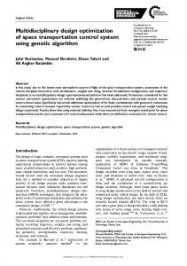
xvi A.5 The AircraftNoise sub-assembly model containing the low-speed aerodynamics model, high-lift system design constraints, aircraft noise design constraints, and aircraft noise analysis model. . . . . . . . . . . . . . . . 127 A.6 The optimization tool window showing the objective function, design constraints, and design variables and their lower and upper bounds. . . . . . 128 A.7 The Data Explorer window which is used to monitor the optimization convergence history. . . . . . . . . . . . . . . . . . . . . . . . . . . . . . . 129 A.8 Convergence history for the reference configuration used in the TE flap noise study in section 4.2. . . . . . . . . . . . . . . . . . . . . . . . . . . 130 A.9 Convergence history for the ∆N = 1 dB noise reduction of the reference configuration (shown in Figure A.8). . . . . . . . . . . . . . . . . . . . . 131 A.10 An example alpha-plot showing constraints for range (which is violated), second segment climb gradient, stability and control, along with the constraint violation criteria. . . . . . . . . . . . . . . . . . . . . . . . . . . . 134 A.11 An example of a parametric study, showing code output before and after bug fixes. . . . . . . . . . . . . . . . . . . . . . . . . . . . . . . . . . . . 134 A.12 Lift curves of a DC-9-30-like aircraft. Based on data from Shevell [8]. . . 136 A.13 Conditions for noise analysis of DC-10 at approach. . . . . . . . . . . . . 138 B.1 The effects of leading edge slats and trailing edge flaps on the wing lift curve. . . . . . . . . . . . . . . . . . . . . . . . . . . . . . . . . . . . . . 140 B.2 Variation of span factor Kb with flap span. . . . . . . . . . . . . . . . . . 141 B.3 A schematic showing how the value of flap span factor Kb is obtained and the definition of Swf . . . . . . . . . . . . . . . . . . . . . . . . . . . . . . 142 B.4 Variation of flap chord factor Kc with wing aspect ratio AR and flap lift factor αδ . . . . . . . . . . . . . . . . . . . . . . . . . . . . . . . . . . . . 144 B.5 Theoretical flap lift factor. . . . . . . . . . . . . . . . . . . . . . . . . . . 145 B.6 Flap effectiveness factor for a double slotted, fixed vane flap. Curve based on experimental data from Torenbeek [7]. . . . . . . . . . . . . . . . . . . 146
xvii C.1 Analysis of a BWB-450-like aircraft with a mission of 478 passengers and 8,700 nm range at cruise Mach 0.85. . . . . . . . . . . . . . . . . . . . . . 149
List of Tables 3.1
Design variables for cantilever wing aircraft . . . . . . . . . . . . . . . . .
33
3.2
Design variables for Strut-Braced-Wing aircraft . . . . . . . . . . . . . .
34
3.3
Design constraints
. . . . . . . . . . . . . . . . . . . . . . . . . . . . . .
35
3.4
BWB design variables . . . . . . . . . . . . . . . . . . . . . . . . . . . .
49
3.5
BWB design constraints . . . . . . . . . . . . . . . . . . . . . . . . . . .
49
3.6
BWB design parameters . . . . . . . . . . . . . . . . . . . . . . . . . . .
50
4.1
Results of the approach speed study. . . . . . . . . . . . . . . . . . . . .
71
4.2
Results of the TE flap noise reduction study. . . . . . . . . . . . . . . . .
85
4.3
Design details for the optimized cantilever wing and Strut-Braced wing aircraft. . . . . . . . . . . . . . . . . . . . . . . . . . . . . . . . . . . . . 100
4.4
Active design constraints. . . . . . . . . . . . . . . . . . . . . . . . . . . 101
4.5
Aircraft characteristics. . . . . . . . . . . . . . . . . . . . . . . . . . . . . 101
4.6
Airframe noise analysis with ANOPP of the optimized aircraft. . . . . . . 101
5.1
An outline of a MDO study of intermediate distributed propulsion effects. Table key: CP = Conventional Propulsion, DP = Distributed Propulsion, PM = Pylon Mounted, BLI = Boundary Layer Ingesting Inlet. . . . . . . 104
5.2
Optimum configuration comparisons between the conventional propulsion and distributed propulsion BWB designs, along with intermediate optimum designs showing the individual distributed propulsion effects. . . . . 108 xviii
xix A.1 Analysis of a B777-200ER-like aircraft. Percentage difference with publicly available data is presented where available. . . . . . . . . . . . . . . . . . 135 A.2 A comparison of lift curve properties with flight test data of DC-9-30 (data from Shevell [8]). . . . . . . . . . . . . . . . . . . . . . . . . . . . . . . . 137 A.3 Airframe noise analysis with ANOPP of DC-10 at approach. . . . . . . . 138 B.1 Coefficients for response surfaces of the flap span effectiveness factor (Kb ), the flap chord factor (Kc ), and the flap effectiveness factor (ηδ ). . . . . . 143 C.1 Weight analysis of a BWB-450-like aircraft with a mission of 478 passengers and 8,700 nm range at cruise Mach 0.85. . . . . . . . . . . . . . . . 148
Nomenclature AR
Aspect ratio
CD
Drag coefficient
CDi
Induced drag coefficient
CDiDP
Distributed propulsion induced drag coefficient
CDp
Profile drag coefficient
CDw
Wave drag coefficient
CJ
Jet momentum flux coefficient =
J 1 2 S ρU∞ ref 2
CL
Lift coefficient
CLapp
Approach lift coefficient =
CLmax
Wland qSref
Maximum lift coefficient =
M T OGW qSref
CLmaxlimit
Maximum theoretical lift coefficient for a given type of high-lift system
L/D
Lift to drag ratio
M
Mach number
M T OGW
Maximum Take-Off Gross Weight
Nref
Reference aircraft configuration noise level
Nnew
New aircraft configuration noise level
∆N
Target noise reduction
Sf
TE flap surface area
Sref
Wing reference area
sf c
Specific fuel consumption
t
Air temperature at a given altitude
T
Total thrust from engine xx
xxi = Tbleed + Texcess Tbleed
Bleed part of thrust from engine
Texcess
Excess part of thrust from engine
Tjet
Jet thrust = ηd Tbleed
Tnet
Bleed part of thrust from engine = Tjet + Texcess
T0
Maximum sea level static thrust
T OGW
Takeoff gross weight
U∞
Free stream velocity
Vmin
Minimum velocity at approach
V
Aircraft speed
Wland
Aircraft landing weight
wd
Duct weight factor
q
Dynamic pressure = 1/2ρV 2
ρ
Air density
δf
TE flap deflection
α
Angle of attack
αapp
Approach angle of attack
αstall
Stall angle of attack
αlimit
Maximum allowable angle of attack = θts − γgs
θts
Tail scrape angle
γgs
Glide slope angle
ηd
Duct efficiency
ηDP
Distributed propulsion factor
ηP
Froude propulsive efficiency
ηT
Engine internal thermal efficiency
κl
sf c factor
Λ
Wing quarter chord sweep angle
Θ
Ratio of jet thrust to net thrust =
Tjet Tnet
≡
CDp +CDw CD
Chapter 1 Introduction The goal of aircraft design is to achieve safe and efficient flight. In the world of commercial air transport, efficient, economically attractive configurations are needed. Therefore, all transport aircraft are designed for high performance and low cost and to meet any required constraints. Environmental and noise constraints are becoming increasingly more important. However, these constraints are generally not included in the early stages of the aircraft design process, except for the most recent Airbus 380 and the soon to come Boeing 787 and Airbus 350. Usually, aircraft have been designed to meet performance and weight goals and then adjusted to satisfy the environmental and noise requirements at the later stages in the design process. Due to the coupled nature of the design it is clear that to meet all the required constraints as well as achieving the best possible solution, all the different disciplines and constraints need to be considered simultaneously. Multidisciplinary Design Optimization (MDO) has been receiving increased interest in the aerospace industry as a valuable tool in aircraft design [9, 10]. The use of MDO in conceptual and preliminary design of aircraft provides the designer with better insight into the coupled nature of different aerospace disciplines related to aircraft design which then lead to improved aircraft performance and faster design cycle time. In a general MDO aircraft design framework, different analysis modules or their surrogates representing the different disciplines, such as structures and aerodynamics, are coupled with an optimizer to find an optimum design subject to specified design constraints. This provides a means of designing aircraft requiring tightly coupled technologies. Furthermore, MDO is the ideal tool to study the effects of introducing new technology or new design constraints 1
2 to conventional aircraft, as well as the design of unconventional aircraft. MDO has been successfully used at the Multidisciplinary Design and Analysis (MAD) Center at Virginia Tech (VT) to study advanced aircraft concepts such as the Strut-Braced Wing aircraft [6, 11] and the Blended-Wing-Body aircraft [3]. Noise, defined as an unwanted sound disturbance, is described mathematically on a logarithmic scale. Therefore, a reduction in one aircraft noise source will have an insignificant effect on the overall noise. So, in order to reduce the overall aircraft noise, all of the noise sources that are of the same magnitude, need to be reduced by the same amount. For example, if noise due to the engines, landing gear, and slats are all 90 dB and those are the only noise sources being considered, then the overall noise is equal to 10log10 (3 × 1090/10 ) = 94.77 dB. If slat noise is reduced by 5 dB, then the overall noise is 10log10 (1085/10 + 2 × 1090/10 ) = 93.65 dB, which is only a 1.12 dB reduction. If the slat noise is eliminated, then the overall noise is 10log10 (2 × 1090/10 ) = 93.01 dB. This is a simplified analysis, since there is some interference between the noise sources. Nonetheless, it clearly demonstrates the need to reduce all the noise sources by the same amount to achieve any significant overall noise reduction. The work presented in this dissertation deals with how to use MDO to design aircraft, at the conceptual design level, for low-noise signature. To observe differences in performance and weight associated with the resulting changes in the aircraft configuration to attain a lower noise level, both conventional and unconventional transport aircraft are studied. These include the conventional cantilever wing configuration, a Strut-BracedWing aircraft, and Blended-Wing-Body aircraft with both conventional propulsion and distributed propulsion.
1.1
Advanced Transport Aircraft Concepts
In this section the advanced aircraft configurations considered in this dissertation are presented, starting first with the typical commercial transport aircraft configuration, the swept cantilever wing concept.
3
1.1.1
Cantilever Wing
Liebeck [12] provides the following insight into the aircraft design evolution. The first powered controlled flight was by the Wright brothers in 1903. About 44 years later, the swept-wing Boeing B-47 took flight. Another 44 years go by, and the Airbus A330 takes off. The comparison of these aircraft, given in Figure 1.1, depicts the evolution of aircraft design in the last century and the focus toward what is regarded as the most efficient configuration.
Figure 1.1: Aircraft design evolution, the first and second 44 years. This also shows a remarkable engineering accomplishment, especially in the first 44 years. The B-47 and A330 embody the same fundamental design features of a modern subsonic jet transport: swept wing and podded engines hung on pylons beneath and forward of the wing. In the second 44 years, the configuration did not changed much, it has only matured and become more efficient by incorporating advanced technology in various components. The most recent aircraft designs that apply this configuration concept are the Airbus A380 and the ultra-long-range Boeing 787. Figure 1.2 shows a typical modern cantilever wing aircraft.
4
1.1.2
Strut-Braced-Wing
A Strut-Braced Wing aircraft configuration has a high-fuselage-mounted wing and a strut between the wing and the fuselage (Figure 1.3). The strut carries a part of the load, and therefore allows the main wing to be thinner and have a higher aspect ratio while not incurring a weight penalty compared to a cantilever wing concept. This permits a significant increase in aerodynamic performance. Compared to an optimized cantilever aircraft with a mission of 7,500 nm and 325 passengers, the SBW aircraft will be, depending on the placement of the engines, about 10-20% lighter and require approximately 14-24% less fuel [6, 11, 13, 14].
1.1.3
Blended-Wing-Body
The Blended Wing Body (BWB) (Figure 1.4) is a relatively new aircraft concept that has potential use as a commercial or military transport aircraft, cargo delivery, or as a fuel tanker. The BWB is basically a flying wing with the payload, i.e., passengers and cargo, enclosed in the thick, airfoil shaped, center section. Studies have shown large potential performance improvements for the BWB over a conventional subsonic transport configuration based on equivalent technology [12, 15]. The BWB concept was introduced by Robert Liebeck at the McDonnel Douglas Corporation (now the Boeing Company) in 1988. The airplane concept blends the fuselage, wing, and the engines into a single lifting surface, allowing the aerodynamic efficiency to be maximized. The biggest improvement in aerodynamic efficiency, when compared to a conventional aircraft, comes from the reduced surface area and thereby reduced skin friction drag. According to Liebeck [12], it is possible to achieve up to a 33% reduction in surface area. This reduction comes mainly from the elimination of tail surfaces and engine/fuselage integration. Clearly, the BWB shows a significant advantage over a conventional aircraft in terms of performance and weight. However, the BWB is a revolutionary aircraft concept and will require a large and expensive engineering effort to become a reality. Most likely, before being used as a transport aircraft, it will be utilized for military applications. In fact, Boeing and the US military are designing the BWB to be used as an advanced tactical transport and as an air refuel tanker (Figure 1.4).
5
Figure 1.2: A typical cantilever wing aircraft with under-the-wing installed engines. A configuration used by most of today’s commercial transport aircraft.
Figure 1.3: A Strut-Braced-Wing aircraft with fuselage mounted engines.
6
Figure 1.4: A Blended-Wing-Body aircraft with Boundary Layer Ingestion (BLI) Inlet Engines (figure by NASA).
1.2
The Distributed Propulsion Concept
Distributing the propulsion system using a number of small engines instead of a few large ones could reduce the total propulsion system noise [16]. There are other potential benefits of distributed propulsion. One advantage is its improved safety due to engine redundancy. With numerous engines, an engine-out condition is not as critical to the aircraft’s performance in terms of loss of available thrust and controllability. The load redistribution provided by the engines has the potential to alleviate gust load/flutter problems, while providing passive load alleviation resulting in a lower wing weight. There is also the possible improvement in affordability due to the use of smaller, easily-interchangeable engines. Ko et al. [1, 2, 3] suggested a distributed propulsion arrangement that is a hybrid of conventional propulsion, jet-wing, and a jet-flap. The configuration involves replacing a small number of large engines with a moderate number of smaller engines and ducting part of the engine exhaust to exit out along the trailing edge of the wing. Figures 1.5 and 1.6 show schematically the general arrangement of this configuration. During cruise, an increase in propulsive efficiency is attainable with this arrangement as the trailing edge jet
7 ‘fills in’ the wake behind the body, improving the overall aerodynamic/propulsion system, resulting in an increased propulsive efficiency. Dippold [17] and Walker [18] performed numerical studies of the jet-wing distributed propulsion arrangement and showed an improvement in propulsive efficiency can be attained with such an arrangement. At take-off and landing, the deflected trailing edge jet replaces the elevons for longitudinal control.
Figure 1.5: A planform view of a BWB with distributed propulsion configuration as proposed by Ko et al. [1, 2, 3].
8
Figure 1.6: Wing streamwise cross-sections at a location with an engine and at a location between engines (from Ko [1]).
9
1.3
Aircraft Noise
Civil transport aircraft must be certified in terms of noise levels set by the FAA in FAR Part 36 [19] and ICAO in Annex 16 [20]. For certification, the noise is measured at three different locations near the runway (Figure 1.7). Those are at • flyover, which is 6.5 km from the brake release point and under the take-off flight path where the aircraft is climbing with reduced power, • the highest measurement recorded at the sideline (450 m from the runway axis) during take-off with max take-off rating, • and at approach, which is 2 km from the runway threshold and under the flight path, with the aircraft at 120 m altitude and 3 degree glide slope, and the aircraft is in its noisiest configuration with landing gear extended and full flap deflection.
Figure 1.7: ICAO and FAR noise certification points. Based on aircraft maximum take-off weight and the number of engines, the Effective Perceived Noise Level (EPNL) is limited by FAA and ICAO regulations. The current and future FAR approach noise level limits are shown in Figure 1.8, along with measured approach noise levels for typical jet-propelled transport aircraft. In addition to these constraints, regulations limit the hours and the number of operations at most airports. There has been approximately a 100% increase in the number of noise related restrictions
10 in the last decade, and the number of airports affected by these noise restrictions has grown significantly worldwide [5]. NASA’s goal is to reduce aircraft noise by 10 decibels by the year 2007 [21] to meet the more stringent noise levels and regulations. This goal is scientifically demanding, because it means reducing the acoustic power by 90% [22]. NASA’s long term goal, within the next 20 years or so, is to reduce aircraft noise by 20 decibels. It is clear that to achieve these noise reduction goals a significant research effort is required. However, if the aircraft can be designed/modified so that it has some leeway within these constraints, airlines can gain improvement in their operations and relief will be provided to the airport’s surrounding community. This gives strong incentive for reduction in aircraft noise. 110
105
B747-400 B757-300 B767-400 B777-200 A300 A310-304 A320-214 A330-322 A340-212 Beechjet 400 Cessna Citation II Bombardier CL-600
Approach Noise (EPNdB)
Stage 3
100
95
-10 EPNdB Stage 4
90
85 10
100 MTOGW (1000 lbs)
1,000
Figure 1.8: Approach noise levels of jet propelled aircraft. Shown is the current approach noise level limit, Stage 3, and the next noise level limit, Stage 4. The data is from FAA Advisory Circular [4]. Smith [23] defines aircraft noise as unwanted sound that is generated whenever the passage of air over the aircraft structure or through its power-plants causes fluctuating pressure disturbances that propagate to an observer in the aircraft or on the ground below.
11 Aircraft main noise sources are the engines, the airframe, and the interference between the engines and the airframe. High-bypass ratio turbofan engines were introduced in the ’60s, and they have been the most important factor in reducing aircraft noise by approximately 20 decibels. Moreover, during take-off and flyover, when the engines develop maximum power, the engines are still the dominant noise source. The self-generated noise from the airframe is normally significant only during the approach. For this reason, airframe noise has been thought of as the ultimate aircraft noise “barrier” [23]. The work presented in this dissertation will focus on how to design aircraft for low airframe noise. For simplicity’s sake, engine noise will not be covered. For details on engine noise, the reader is referred to Smith [23] and Hubbard [24].
1.3.1
Airframe Noise
Airframe noise sources on a conventional transport are the landing gear, trailing edge (TE) flaps, leading edge (LE) slats, the clean wing, and the tail surfaces [25] (Figure 1.9). The leading-edge slats, flap edges, and the landing gear are the major contributors to airframe noise and the main landing gear is the dominant noise source on most modern wide-body transports [26] (Figure 1.10).
Figure 1.9: Airframe noise sources (from Hosder [5]). The landing gear assembly has a large number of components that vary in shape, size and orientation. Associated with the landing gear is also the wheel-well cavity. The flow past the gear assembly is turbulent, unsteady, separated and highly three-dimensional.
12 This flow is the source of landing gear noise, and it varies with approximately the sixth power of the aircraft speed [23]. The flow in the wheel-well cavity is mainly tonal and since the size of the gear components vary greatly, the noise spectrum is broadband [22].
Figure 1.10: Dominant airframe noise sources for conventional aircraft. High-lift systems are necessary to allow airplanes to take-off and land on runways of acceptable length without penalizing the cruise efficiency significantly [27, 28]. Leading edge slats are used to delay separation on the wing at high lift conditions to allow for increased angle of attack and a corresponding increase in maximum lift coefficient. Slat noise is closely related to the local slat/slot flow characteristics. The flow field in the slat region is characterized by high local velocities at the leading-edges of both the slat and the main wing, a vortex flow in the back side cove and an accelerated flow in the slot between the slat and the wing leading-edge [29]. The main source of slat noise comes from the region close to the slat trailing-edge, where resonance between the vortex shedding from the trailing-edge of the slat and the gap between the slat and the main wing [30]. This part of slat noise is tonal. Lilley [25] says that by changing the slat gap and overlap, it is possible to detune the system to avoid resonances, but at the expense of reducing the aerodynamic efficiency of the high-lift system. Instabilities in the cove shear layer produce the broadband component of the slat noise [22]. Flap noise originates from the flap trailing edges and flap side edges [25]. Due to the sharp change in lift between the flapped and unflapped portion of the wing at high-lift
13
Figure 1.11: A streamwise cut of a wing with high-lift system comprising of a leading edge slat and a trailing edge slat. conditions, a strong vortex is formed at the flap side edge, and that is why the flap side edge noise is the dominant flap noise source [22]. A clean wing is defined as the configuration that has all the high-lift devices and the undercarriage in stowed positions. The main noise mechanism for a clean wing is trailingedge noise, which originates from the scattering of the acoustic waves generated due to the passage of turbulent flow past the sharp wing trailing edge. The far-field noise intensity of trailing-edge noise varies approximately with the 5th power of the velocity [23].
1.3.2
Noise Abatement Procedures
Changing the flight path and/or the speed of the aircraft during flyover and approach is the most obvious way of reducing aircraft noise without modifying the aircraft itself. Airframe noise is an inverse function of the square of the distance from the source to the observer. Also, airframe noise varies approximately as the 5th power of the speed. Combining these effects, the approximate noise reduction for aircraft at approach that can be obtained from changing the altitude and speed can be calculated as [22] � N oiseReduction = 10log10
V Vref
�5 �
rref �2 , r
(1.1)
where V is the speed of the aircraft, r is the distance from the aircraft to the observer, and ref refers to normal approach values. This shows that approximately 3.1 dB noise reduction can be achieved if the aircraft flies 10% higher and 10% slower at approach. If the speed is kept constant, a 43% increase in altitude is required to obtain a 3.1 dB noise
14 reduction. Only a 13% reduction in speed is required to obtain the same noise reduction if the altitude is kept constant. Clearly, the speed reduction is more effective in reducing the airframe noise. However, for lower approach speeds the aircraft will have to increase the angle of attack to meet the required lift and/or increase the flap deflection. This will increase the drag, and therefore the thrust must be increased, which leads to an increase in engine noise. Finding the “best” trade-off between velocity and distance so that an optimal flight path can be found should be addressed by using optimization, such as the study presented by Zou and Clarke [31].
1.3.3
Add-On Treatments
Landing Gear One way to reduce landing gear noise is to add a fairing of some sort around the landing gear to make it’s shape more aerodynamic. This would reduce the separation and the strong shedding, which is the main source of noise. Lockard and Lilley [22] mention two types of fairings, a rigid fairing and a virtual fluidic fairing, like blowing. Both of these fairings would increase the complexity of the landing gear, but could reduce the noise significantly. Much research on landing gear noise is currently underway [32, 33, 34, 35]. Piet et al. [33] reported a 1.8 EPNdB landing gear noise reduction on an A340-300 aircraft by using fairings. Dobryzynski et al. [34] designed and tested low-noise landing gears of A340 type. Relative to the conventional landing gears, a reduction of broadband landing gear noise of the order 5 to 6 dB was achieved. They conclude that the main reason for today’s landing gear noise problems is the increase in the length of the landing gears. This is due to the continuous increase in high bypass ratio engine/nacelle diameter and the requirement to maintain engine-to-ground clearance for an under-the-wing engine installation. Therefore, the 10 dB noise reduction goal will not be reached with conventional landing gear configuration, and the development of fuselage mounted short landing gears should be considered for future aircraft.
15 High-Lift Systems Flap side edge noise can be reduced by disrupting and/or moving the vortex system by using the following methods [22]: • A porous flap tip smoothes out the transition from the flapped region to the unflapped region by allowing the pressure and suction side to diffuse the tip vortex and reduce the sharp change in lift. • A Continuous Moldline Link (CML) bridges the gap between the flapped region and the unflapped region and helps reduce the sharp change in lift much like a porous flap tip. The expected flap noise reduction in EPNL is over 5 dB [22]. • A fence moves the vortex away from the flap tip. A fence works similarly as a winglet [36]. This configuration has a cruise performance penalty. • Side-edge Blowing has the potential of moving and diffusing the vortex system, but will add complexity to the high-lift system. Slat noise noise can be reduced by using the following [22]: • By thinning the slat trailing edge the noise can be eliminated. • Vortex generators change the boundary layer thickness on the slat and could be effective in reducing the slat noise. • A porous slat could reduce the unsteadiness in the cove region and significantly affect the slat cove noise. • By filling the cove region the noise can be reduced.
1.3.4
Designing Aircraft for Low-Noise
Caves et al. [37, 38] developed a model that integrates a conceptual aircraft design model with the NASA Aircraft Noise Prediction Program (ANOPP) [39]. The model was used to study the effect of changing the thrust/weight ratio on the take-off flyover noise levels
16 and the sensitivity of approach angle to approach noise levels. Results showed that increasing the altitude during approach phase will significantly reduce approach noise. Antoine et al. [40, 41, 42, 43] used MDO to design the aircraft and mission to meet specified noise constraints at flyover, sideline, and approach conditions. Abatement procedures such as steeper approaches and thrust cutback on take-off were also included in the analysis. The results showed that engine bypass ratio was a driving factor in reducing engine noise. Furthermore, steeper approaches can effectively reduce approach noise. The BWB has been recognized as the ultimate low-noise aircraft configuration [5, 12, 44]. NASA [45, 46, 47] has done research on propulsion-airframe-aeroacoustic technologies for a BWB aircraft with an array of small turbofan engines which focused on reducing engine noise. Manneville et al. [48] studied BWB aircraft with a distributed propulsion system with multiple ultra-high bypass ratio engines and reported a 30 dB reduction in jet noise could be attainable with such a configuration.
1.4
Contributions of the Current Study
This research deals with how to design low-noise transport aircraft using MDO. The subject is approached in two ways. One way explicitly designs low-airframe-noise transport aircraft. This involves optimizing aircraft to minimize maximum-take-off-weight, while constraining noise at approach condition. A methodology is presented describing how to incorporate noise as an objective function and as a design constraint in the optimization formulation. The other way, implicitly designs low-noise aircraft, which involves choosing a configuration supporting low-noise operation and optimizing its design, not considering any aircraft noise during the procedure. To achieve the objective, two MDO frameworks were designed and developed. The framework used for the explicit design procedure was constructed using available aircraft and noise analysis computer codes, as well as designing new ones. The framework used for the implicit design procedure was initially developed by Ko [1], but here it has been improved and developed further to give more accurate and realistic aircraft designs. The guiding modeling philosophy behind the design of these frameworks is explained in detail. To explicitly design for low-airframe-noise, a typical modern transport aircraft (a can-
17 tilever wing aircraft) and a SBW aircraft are studied and compared. For the implicit design procedure, the effects of distributed propulsion on a BWB aircraft are studied.
1.5
Outline of the Dissertation
An outline of the dissertation is given if Figure 1.12. The design methodology for incorporation of noise into an MDO formulation is presented in Chapter 2. A detailed description of two MDO frameworks are given in Chapter 3. The first framework described is capable of optimizing both cantilever wing and SBW aircraft including noise constraints. The second framework can optimize BWB aircraft with distributed propulsion. Chapter 4 presents airframe noise reduction design studies of cantilever wing and SBW aircraft. A design study of the effects of distributed propulsion on BWB aircraft is presented in Chapter 5. The results are summarized and discussed in Chapter 6. Three appendices are included. Appendix A includes a user guide to the airframe noise reduction MDO model and results of validation. Appendix B gives details of a low-speed aerodynamics model used in the noise reduction MDO model. Appendix C gives results of validation studies for the BWB MDO model.
Figure 1.12: Outline of the Dissertation.
Chapter 2 Design Methodology Aircraft noise minimization can be approached in three ways: (1) by explicitly designing for low-noise, (2) by implicitly designing for low-noise, and (3) a combination of (1) and (2). By incorporating noise constraints into the design process, the aircraft is explicitly designed to meet required noise levels. The aircraft is implicitly designed for low-noise by selecting a configuration with features which support a low-noise operation. Of course the two approaches can be combined in the design of aircraft. A methodology for explicitly designing low-noise aircraft using Multidisciplinary Design Optimization (MDO) is presented in this chapter.
2.1
Implicit Design
A configuration that has the potential for significant reduction in environmental emissions and noise is the Blended-Wing Body (BWB) aircraft [12] (Figure 1.4). The key features that make the BWB a good candidate for low-noise low-emissions aircraft are: • The engines are located on the upper surface of the aircraft, and therefore the forward-radiated engine fan noise is shielded by the centerbody and the engine exhaust noise is not reflected by the lower surface of the wing [49]. • The BWB has a large wing area and does not require trailing edge flaps, since it can approach and land at a low lift coefficients. Therefore, a major source of airframe 18
19 noise is eliminated. However, the BWB uses elevons for longitudinal control which should generate noise, but possibly significantly less than trailing edge flaps. • The BWB is well suited for the use of the distributed propulsion concept (see section 1.2). With smaller engines a reduction in jet noise can be attained [45, 46, 47]. • Lower total installed thrust and lower fuel burn imply an equivalent reduction in engine emissions, using the same engine technology. It seems that the BWB offers a significant reduction in emissions and noise without any specific acoustic treatment. Another configuration that has the potential of reduction in weight, fuel consumption, emissions and noise is the Strut-Braced Wing (SBW) aircraft (Figure 1.3). As mentioned in section 1.1.2, the SBW aircraft can be designed to be about 10-20% lighter, and require approximately 14-24% less fuel than a cantilever wing aircraft at a comparable technology level. The total weight reduction depends on the placement of the engines, i.e., whether the engines are installed under the wing, which will provide wing load alleviation, or on the fuselage, which will not provide wing load alleviation. However, by having the engines mounted on the fuselage, the landing gear can be designed to be smaller by mounting it on the fuselage. A large reduction in landing gear noise can be achieved by designing it to be smaller and simpler [34]. Since the strut is used to alleviate the wing loading, the wing can still be designed to be thin and light although the engines may not necessarily be mounted on the wing for load alleviation.
2.2
Explicit Design
In general, the addition of aircraft noise into a MDO formulation for conceptual aircraft design can be approached in two ways. Aircraft noise can be an objective function that is to be minimized, or a design constraint that needs to be met.
2.2.1
Noise as an Objective Function
Commonly used objective functions in MDO for aircraft are: minimize Take-Off Gross Weight (T OGW ), maximize range, or minimize Direct Operating Cost (DOC). To
20 observe the changes in the aircraft systematically if noise is an objective function, a constraint is needed on one of the aforementioned functions. That is, if one wants to minimize the noise but allow only a 1,000 lb penalty in weight, a constraint should be added that limits the increase in T OGW by that amount. This way, a relation between noise reduction and the change in T OGW can be found by systematically increasing the allowable T OGW penalty (∆T OGW ) and optimizing the aircraft for each step.
Figure 2.1: A procedure to optimize aircraft for minimum noise (N ) while limiting the weight penalty with respect to a conventionally optimized configuration. The procedure to optimize aircraft for minimum noise while limiting the weight penalty is as follows (Figure 2.1). Start by optimizing the aircraft for minimum T OGW subject to the conventional design constraints. The optimized aircraft is the reference configuration with the reference weight T OGWref . For the next step, make noise the design objective and add a design constraint on T OGW that limits it by a weight penalty ∆T OGW . The design constraint can be written as
T OGWnew ≤ T OGWref + ∆T OGW.
(2.1)
Now, the reference configuration can be re-optimized for minimum noise subject to all the
21 same design constraints as before (as discussed in section 3.3.2), but with the additional constraint on T OGW . The weight penalty ∆T OGW can be successively increased and the aircraft re-optimized to obtain the change in weight and performance with reduced noise.
2.2.2
Noise as a Design Constraint
Minimal changes are needed to the MDO formulation if the aircraft noise is added as a design constraint. A sensible approach to this problem is to start by optimizing the aircraft for minimum T OGW subject to the conventional design constraints without considering noise. This will give an aircraft that is conventionally designed and optimized to be used as the reference configuration. The next step is to analyze the reference configuration at the desired flight condition (in our case at approach) to obtain a reference noise level (Nref ). Now, a design constraint can be added to the MDO formulation that will require a target noise reduction (∆N < 0) compared to the reference noise level. This design constraint can be written as
Nnew − Nref ≤ ∆N,
(2.2)
where Nnew is the noise level of the new configuration. The final step is to re-optimize the reference configuration with the same MDO formulation as before except with the added noise constraint. A new configuration will be obtained that has ∆N less noise. This procedure is shown in Figure 2.2. As discussed in the beginning of this chapter, to reduce the overall aircraft noise, each of the dominant noise sources need to be reduced simultaneously by the same amount. In order to achieve this goal using MDO, the airframe noise models need to be modeled appropriately to reflect the changes in the aircraft configuration. Since ANOPP will be used for airframe noise analysis, the available models need to be reviewed and discussed further before implementing them in the MDO formulation.
22
Figure 2.2: A procedure to optimize aircraft for a target noise reduction (∆N ) compared to a reference noise level (Nref ) of a conventionally optimized reference configuration.
2.2.3
Designing for Low-Airframe-Noise using ANOPP
The objective of the current study is to observe the changes in aircraft geometry, weight, and performance when considering airframe noise in the conceptual design of aircraft with MDO. It is clear from the overview in section 3.3.4 of the airframe noise models employed in ANOPP that not all of them are appropriate for use in MDO. A closer look at these models is, therefore, required before deciding on how to use them in the MDO formulation. Although the landing gear noise is currently the most dominant airframe noise, the landing gear noise model in ANOPP is not appropriate for use in the design optimization since it is a function of landing gear geometry (see section 3.3.4), which is generally not included in the design optimization of the entire aircraft. Design of the landing gear is an entirely separate problem in itself, and much research is being conducted on landing gear noise reduction [32, 33, 34, 35]. However, the landing gear model can be used when performing an off-line noise analysis of aircraft. The three remaining airframe noise models (LE slat, the clean wing, and TE flap) are
23 all related to the wing and tail surfaces of the aircraft. The noise of the high lift devices (LE slat and TE flap) are more dominant than the clean wing noise. The LE slat noise and TE flap noise are comparable. Furthermore, these three aerodynamic devices are all interconnected. The wing design is based on the weight of the aircraft, the required performance, and the design constraints. The required size and function of the highlift devices (LE slats and TE flaps) depend on the high-lift requirement at approach conditions and the size of the wing. Therefore, by reducing the high-lift requirement at approach it is possible to reduce or eliminate noise due to the high-lift devices. This means that by increasing the wing size, the high lift devices can be simplified, reduced in size or eliminated entirely. However, with the increased wing size, aircraft performance will be penalized. Clearly, MDO can, and should, be used to study the effect of increasing the wing size to reduce the high-lift requirement, thereby reducing noise associated with the high-lift devices. The LE slat noise model in ANOPP assumes a fixed geometry of the slat (15% slatchord to wing-chord ratio and full slat-span to wing-span). In MDO then, the aircraft wing geometry has to be changed to change the LE slat noise. The TE flap noise model is proportional to the flap area (Sf ) and proportional to the sine squared of the flap deflection (δf ). The TE flap noise model is constructed in a way that permits use in MDO. The size of the flap and the flap deflection can be designed with MDO so that the TE flap noise is reduced while still meeting the lift requirements at the approach condition. The clean wing TE noise is a function of the wing geometry and is also appropriate for use in MDO. LE slats are used to delay separation on the wing at high-lift conditions to allow for increased angle of attack and a corresponding increase in maximum lift coefficient. TE flaps increase the lift at zero angle of attack and also increase the maximum lift coefficient. So, the increased lift comes from deflecting the TE flaps and the deployment of the LE slats increases the possible angle of attack. Therefore by simplifying and/or reducing the size of the TE flaps, the high-lift capability is reduced and the wing area needs to be increased to meet the required high lift requirements due to FAR design requirements (CLmax ≥ 1.32 CLapp ). Furthermore, it is possible to eliminate the use of LE slats if the wing is large enough to carry all the lift and still have a high enough maximum lift coefficient to meet the design requirement.
24 TE Flap Noise Study Based the above discussion, and the limitations of the available airframe noise models in ANOPP, the following TE flap noise study is proposed. The objective of the study is to reduce or eliminate TE flap noise by reducing the high-lift requirement. Only TE flap noise is included in the optimization process. Other noise sources, such as the engines, the landing gear, LE slats, and the clean wing are not included in the optimization. An offline analysis is performed before and after each optimization run to monitor the changes in the other noise sources. However, it should be noted here that any noise reduction in TE flap noise will only matter to the overall aircraft noise if the other dominant noise sources (the engines, landing gear, LE slats) are reduced by the same amount.
Figure 2.3: An outline of the TE flap noise study. An outline of the proposed TE flap noise study is given in Figure 2.3. The MDO formulation is set up as discussed in section 3.3.2. We will minimize T OGW with respect to design variables in Table 3.1 (or Table 3.2 in the case of a SBW aircraft) subject to the design constraints in Table 3.3. With this formulation, a conventionally designed aircraft is obtained. This configuration is used as the reference configuration. The next step is to
25 perform airframe noise analysis to obtain the reference TE flap noise level, Nfref . Now a design noise constraint is added to the MDO formulation that requires a target TE flap noise reduction ∆Nf . The final step is to re-optimize the aircraft. The last step is repeated over and over until an overall desired noise reduction is attained or until any design constraint limits further progress. To save computational time, it is best to use the previous obtained design as a starting point to obtain a design for the next required target noise reduction.
Chapter 3 MDO Modeling This chapter gives the details of the Multidisciplinary Design Optimization (MDO) frameworks designed and developed in this research. The frameworks are intended for design optimization of low-noise aircraft, both implicitly and explicitly. An overview of the work done by the author is given, along with the guiding modeling philosophy, and the objectives for the design of the MDO frameworks.
3.1
Overview
Two different MDO frameworks have been designed and developed. One framework is used for implicitly designing for low-noise aircraft, and the other for explicitly designing for low-airframe-noise. The framework used for implicit design was initially designed and developed by Ko [1]. This framework handles Blended-Wing-Body (BWB) transport aircraft with conventional propulsion and distributed propulsion. The author has successfully improved this framework to yield more accurate and realistic designs. The major improvements are listed in Figure 3.1 and they include MDO formulation refinements, improved description of vehicle hull and geometry, improved wing weight model, engine model, and duct efficiency model, and lastly the addition of a cruise trim drag calculation. The details of these improvements and the BWB MDO framework are covered in section 3.4. The framework intended for explicit design of low airframe noise aircraft was developed 26
27
Figure 3.1: An overview of the major improvements made by the author to a Blended-WingBody transport aircraft MDO framework developed by Ko [1]. by the author. This framework, shown schematically in Figure 3.3, employs an existing aircraft analysis code that is capable of analyzing both cantilever wing and Strut-Braced Wing aircraft that has been developed at Virginia Tech [14]. NASA Langley’s Aircraft Noise Prediction Program (ANOPP) [39] is used for aircraft noise analysis and a code was developed that can handle low-speed aerodynamics of conventional transport aircraft. All these codes are programmed in Fortran except the low-speed aerodynamics code, which is written in Matlab. The ModelCenter software by Phoenix Integration
1
is a visual environment for process
integration and design optimization. The Analysis Server software by Phoenix Integration allows you to “wrap” or convert your design and analysis software into reusable components that can be directly accessed within ModelCenter. The combination of these two tools creates an integration platform for different types of computer codes programmed in different computer languages, such as Fortran, C, C++, and Visual Basic. ModelCenter also provides plug-ins for software such as Matlab, Mathcad, Excel, and CATIA V5. ModelCenter includes an optimizer, which is the Design Optimization Tools (DOT) software by Vanderplaats2 . By using ModelCenter and Analysis Server a framework can be created that allows old and new computer codes to work together. For example, old aerodynamics and structure legacy codes programmed in Fortran can be linked to an optimizer to create an MDO 1 2
Website: www.phoenix-int.com Website: www.vrand.com
28
Figure 3.2: A schematic showing the different analysis codes used to construct an MDO framework capable of performing aircraft design optimization which includes aircraft noise constraints. framework capable of analyzing different types of aircraft. The user can designate which design variables to use, such as wing span and wing chords, as well as design constraints, such as required range and landing distance. Due to the flexible framework provided by ModelCenter, it is also relatively easy to add new analysis modules in the framework, which is convenient when improved or new versions become available, or change the design objective, design variables, and design constraints. Both the frameworks designed and developed in this research use ModelCenter and Analysis Server to integrate the different computer codes. The Method of Feasible Directions (MFD) was used as the optimization algorithm for all the design studies presented in this research.
3.2
Modeling Philosophy
The goals of the present research are mainly twofold. Firstly, to create an MDO framework that can be used for the conceptual design of civil transport aircraft which includes
29 aircraft noise analysis. The framework needs to give accurate enough analysis so it will provide results that reflect the behavior of typical transport aircraft. Secondly, to use the framework to study effects on aircraft design of introducing new technology and/or new design constraints, such as allowable aircraft noise levels at airports. The guiding philosophy behind the modeling and design of the MDO frameworks presented in this research can be summarized as follows: • Keep aircraft analysis on the conceptual design level. • The framework needs to have the capability of analyzing conventional aircraft (cantilever wing) and unconventional aircraft (Strut-Braced Wing and a Blended-WingBody). • Realistic aerodynamic analysis (at high-speed and low-speed), weight analysis, and airframe noise analysis are required. • Analysis should be capable of capturing major design constraints of transport aircraft during take-off, approach, and landing. • Use low- to medium-fidelity analysis models to minimize computational requirements. • Framework needs to be flexible so design objectives, design variables, and design constraints can easily be chosen or changed. In summary, the MDO framework needs to be capable of analyzing both conventional and unconventional aircraft at the conceptual design level in terms of aerodynamics, performance, weight, and airframe noise with enough accuracy to reflect behavior of typical transport aircraft. Furthermore, the framework needs to be in an environment that allows for fast and easy changes to the MDO formulation.
30
3.3
A Model for Explicit Low-Noise Design: MDO of Low-Airframe-Noise Transport Aircraft
An MDO model has been developed that integrates aircraft performance analysis codes and noise analysis codes for the design of both cantilever wing and SBW aircraft (Figure 3.3).
Figure 3.3: An N-squared diagram of the MDO framework. The optimizer used is Design Optimization Tools (DOT) by Vanderplaats. The aircraft analysis code is capable of handling a cantilever wing and a Strut-Braced Wing aircraft [6]. ANOPP is used for airframe noise c analysis. ModelCenter by Phoenix Integration is used to integrate the analysis codes and provides the optimizer. For aircraft performance and weight analysis, a code previously developed at Virginia Tech (VT) was used [6]. This code is capable of optimizing aircraft, but it is used only in analysis mode in the framework. Several modifications and improvements were made to the code during the development, and they are described below. The Aircraft Noise Prediction Program (ANOPP) is a semi-empirical code that uses publicly available noise prediction schemes and is continuously updated by NASA Langely [39]. ANOPP uses “state of the art” noise prediction methods and is the industry standard. Therefore, ANOPP is used in this study for airframe noise analysis.
31
3.3.1
Aircraft Geometric Description
The aircraft is described using a parametric model with a relatively small number of design parameters. The fuselage geometry remains fixed during the optimization. Several input parameters define the geometry, such as the fuselage length and position of wing and tail surfaces (Figure 3.4).
Figure 3.4: Fuselage geometry and parameters. Three spanwise stations are used to define the shape of the wing planform (Figure 3.5). The geometric properties at those stations are design variables. They are chord length, airfoil thickness-to-chord ratio, and the quarter-chord sweep. A straight line wrap method is used to define the properties between the span stations.
Figure 3.5: Wing geometry and design variables
32 In the case of a SBW aircraft, a strut is attached from the fuselage to the wing (Figure 3.6). A telescoping sleeve mechanism allows the strut to be inactive in compression loads (to prevent buckling) and only during positive g conditions does the strut engage. An offset is included at the strut/wing intersection to minimize drag.
Figure 3.6: A schematic showing the wing-strut configuration.
Figure 3.7: High lift system configuration.
33 The high lift system configuration is shown in Figure 3.7. The high lift system is assumed to have leading edge (LE) slats of span bs and a slat-chord to wing-chord ratio of Es constant along the wing span. A continuous trailing edge (TE) flap configuration, with a flap span bf and a constant flap-chord to wing-chord ratio Ef along the wing span, have been chosen. By having a continuous TE flap, the lift-to-drag ratio is maximized and the flap-tip noise minimized. Both the slats and the flaps are located a distance x outboard of the fuselage (set to 1 ft). Ailerons are located outboard of the TE flap with a span ba and a aileron-chord to wing-chord ratio, Ea , constant along the wing span. The ailerons are not high lift devices and are only used for roll-control. They are included here for wing weight calculation.
3.3.2
MDO Formulation
The objective function selected is to minimize Take-Off Gross Weight (T OGW ). The set of design variables and design constraints are different between cantilever wing and SBW aircraft.
Nr. 1 2 3 4 5 6 7 8 9 10 11 12 13 14 15 16 17
Table 3.1: Design variables for cantilever wing aircraft Design Variable Description b/2 Wing semi-span ηb Wing break span station cr Wing root chord cb Wing break chord ct Wing tip chord (t/c)r Wing root thickness to chord ratio (t/c)b Wing break thickness to chord ratio (t/c)t Wing tip thickness to chord ratio Λc/4 Wing quarter chord sweep tskin Wing skin thickness at centerline kvtail Vertical tail scaling factor ηeng Engine spanwise location bf /2 TE flap semi-span Ef Flap-chord to wing-chord ratio Wf uel Fuel weight Tmaxsls Maximum sea level static thrust per engine hcruise Average cruise altitude
Range 90.0 - 132.1 0.2 - 0.9 52 - 100 ft 5 - 50 ft 5 - 50 ft 0.005 - 0.20 0.005 - 0.20 0.005 - 0.20 0 - 40 deg. 0.004 - 2.0 in. 0.5 - 2 0-1 0 - 80 ft 0 - 0.35 100,000 - 400,000 lb 10,000 - 150,000 lb 10,000 - 50,000 ft
34 A total of 17 design variables are used for cantilever wing aircraft (Table 3.1) and they include aircraft geometric properties (main wing, vertical tail, engine location, and high lift system) and operating parameters such as average cruise altitude, maximum sea level static thrust and fuel weight. The flap semi-span (bf /2) and flap-chord to wing-chord ratio (Ef ) were chosen to be the high lift system design variables.
Nr. 1 2 3 5 6 7 8 9 10 11 12 13 14 15 16 17 18 19 20 21 22
Table 3.2: Design Variable b/2 ηint cr ct (t/c)r (t/c)b (t/c)t Λc/4 tskin kvtail cstrut (t/c)strut Λc/4strut ∆xstrut ∆zstrut Fstrut bf /2 Ef Wf uel Tmaxsls hcruise
Design variables for Strut-Braced-Wing aircraft Description Range Wing semi-span 90.0 - 132.1 Wing-strut intersection spanwise location 0.2 - 0.9 Wing root chord 52 - 100 ft Wing tip chord 5 - 50 ft Wing root thickness to chord ratio 0.005 - 0.20 Wing break thickness to chord ratio 0.005 - 0.20 Wing tip thickness to chord ratio 0.005 - 0.20 Wing quarter chord sweep 0 - 40 deg. Wing skin thickness at centerline 0.004 - 2.0 in. Vertical tail scaling factor 0.5 - 2 Strut chord 4 - 20 ft Strut thickness to chord ratio 0.008 - 0.20 Strut quarter chord sweep 0 - 50 deg. Strut chordwise offset 0 - 10 ft Strut vertical aerodynamic offset 1 - 10 ft Strut tension force 0 - 1E6 lb TE-flap semi-span 0 - 80 ft Flap-chord to wing-chord ratio 0 - 0.35 Fuel weight 100,000 - 400,000 lb Maximum sea level static thrust per engine 10,000 - 150,000 lb Average cruise altitude 10,000 - 50,000 ft
A total of 22 design variables are used for SBW aircraft (Table 3.2). Main wing design variables are the same as for cantilever wing, except for the wing break location. The wing break is set to be the same as the wing-strut intersection, and the chord length is interpolated based on the root and tip chord. Design variables for the strut include wing-strut spanwise location, strut chord, thickness-to-chord ratio, quarter chord sweep, chordwise offset, vertical aerodynamic offset, and strut tension force. Design variables for the high lift system and operating parameters remain the same as for cantilever aircraft. The engines are fuselage mounted on the SBW configuration.
35 There are 16 design constraints which cover the aircraft geometry, takeoff, climb, cruise, and landing (Table 3.3). The same constraints are used for both cantilever wing and SBW, except for constraints number 10 and 11, which are only used for cantilever wing aircraft to ensure that there is enough room for the landing gear, which is assumed to be wing-mounted. The landing gear for SBW aircraft are assumed to be fuselage mounted (which will only affect the airframe noise analysis, not the weight estimation). Table 3.3: Design constraints Nr. Constraint Description 1 Range ≥ 7,730 nm 2 Fuel Capacity Fuel Volume ≤ Fuel Tank Volume 3 Balanced Field Length ≤ 11,000 ft 4 Second Segment Climb Gradient ≥ 0.027 5 Missed Approach Climb Gradient ≥ 0.024 6 Rate of Climb at Top of Climb ≥ 300 ft/min 7 Landing Distance ≤ 11,000 ft 8 Engine out Required Cn ≤ Available Cn 9 Section Cl ≤ 0.8 10 Wing break ≥ 32f t 11 Engine spanwise location ≥ 32f t 12 Wing tip deflection at taxi bump ≤ 20f t 13 TE flap tip location ηbo ≤ 0.75 14 Angle of attack at approach ≤ θts − γgs 15 Maximum lift coefficient at approach ≥ 1.32 CLapp (see Eq. (3.1)) 16 Maximum lift coefficient at approach ≤ CLmaxlimit Constraints number 13 to 16 pertain to the high lift system. Constraint 13 ensures that the outboard tip of the trailing edge flap does not exceed 75% of the wing semi-span to allow room for the outboard ailerons. The maximum possible angle of attack is limited by the fuselage tail scrape angle (θts ) and the glide slope angle (γgs ) in constraint number 14. The tail scrape angle is set to 12 degrees and the glide slope angle is assumed to be -3 degrees, giving a maximum possible angle of attack of 15 degrees. FAR Part 25 requires the maximum lift coefficient CLmax at approach to be greater or equal to (1.3)2 CLapp . Constraint 15 makes sure that this condition is fulfilled. Constraint 16 is included as a ‘sanity-check’ for the optimizer. This constraint limits the maximum lift coefficient attainable for the given type of high lift system. In this study, a conventional mechanical-type high lift system is used, and the maximum attainable lift
36
Figure 3.8: A schematic of a typical wing lift curve with TE flap deflection δf ≥ 0. Maximum lift coefficient CLmax is attainable at the stall angle of attack αstall . CLmaxlimit is the maximum attainable lift coefficient at approach for a given type of high lift system (on the order of 3.0). Angle of attack is limited by the fuselage tail scrape angle (θts ) and the glide slope angle (γgs ). coefficient at approach (CLmaxlimit ) is on the order of 3.0. Figure 3.8 graphically shows a typical wing lift curve along with the design constraints applied in this formulation. The flap deflection angle (δf ) required to fulfill the approach lift constraint (constraint 15 in Table 3.3) must be calculated given the flap semi-span and flap-chord to wing-chord ratio (which are set as design variables). The flap deflection angle is found by performing a one-dimensional search between minimum (δflb ) and maximum (δfub ) allowable angles so that the approach lift constraint is fulfilled. Mathematically, this is formulated as
minf (δf ) = |(1.3)2 CLapp − CLmax (δf )|
(3.1)
for δf ∈ [δflb , δfub ], where the lower and upper limits were set as δflb = 0o and δflb = 30o .
37
3.3.3
Aircraft Analysis
In this section the aircraft analysis module is described. This module is based on Virginia Tech’s (VT) previous work on SBW aircraft [6, 11, 14], but the module has been modified and improved here. Major improvements include the addition of a cg calculation and high-lift system analysis.
Mission Profile The mission used in this study is of 305 passengers and 7,730 nm range at cruise Mach 0.85 with 500 nm reserve range (Figure 3.9). The aircraft is assumed to be climbing during cruise at a constant Mach number so that the lift-to-drag ratio stays approximately constant.
Figure 3.9: SBW aircraft mission profile.
High-Speed Aerodynamics By using a combination of traditional aerodynamics estimation methods and response surface models, developed by using Computational Fluid Dynamics (CFD) analysis, an approximate aerodynamic model for cantilever wing and SBW aircraft was developed. The aerodynamic model accounts for parasite, induced, wave and interference drag.
38 The parasitic drag model is based on applying form factors to an equivalent flat plate skin friction drag analysis [50]. The amount of laminar flow on the wing and tails is based on experimental results for commercial aircraft [51, 52]. Transition location on the fuselage, nacelles, and pylons is estimated based on the Reynolds number. The induced drag is determined from a Trefftz plane analysis [53]. The analysis includes the estimated aircraft average cruise cg location (see section 3.3.3) and, therefore, gives the trimmed induced drag. Wave drag is calculated using an extended Korn equation which accounts for wing sweep using Simple Sweep Theory [54]. The drag divergence Mach number is estimated as a function of airfoil technology factor, thickness-to-chord ratio, section lift coefficient, and sweep angle. The wing is divided into several strips (about 16) and the wave drag is estimated for each strip. The total wave drag is the sum of the wave drag for each strip. A response surface model is used to calculate the interference drag of the wing, strut, and fuselage intersections [55]. The response surface model is based on CFD analysis of wing and wing-strut compositions at the cruise Mach number of 0.85. The model gives the drag penalty associated with the strut.
Low-Speed Aerodynamics Airframe noise analysis requires the specification of the high-lift system properties. Therefore, a high lift system analysis module was added to the aircraft analysis. The methods utilized are based on semi-empirical methods provided by Torenbeek [7] and Schemensky [56], both of which are based on methods provided by DATCOM. A detailed description of the low-speed aerodynamics model is presented in Appendix B.
Structures/Weights Two different wing-weight-formulations are available in the weights module. The first one uses NASA Langley’s Flight Optimization Software (FLOPS) [57] to calculate the wing weight and is appropriate for cantilever wing aircraft. The second formulation combines FLOPS with a subroutine that calculates the wing bending material weight. This model was adopted due to the unconventional wing concept of the SBW. The wing bending
39 material weight is calculated using a piecewise-linear beam model, representing the wing structure as an idealized double-plate model and takes into account the influence of the strut on the structural wing design [6]. Weights of the remaining components of the wing are calculated with FLOPS. A detailed description of the wing structures model can be found in [58]. The weight of the individual components of the aircraft, such as the fuselage, tail surfaces, and payload, are calculated using FLOPS.
Propulsion This study assumes a GE-90 class, high-bypass-ratio turbofan engines. Rubber engine sizing is used to scale the engine to meet thrust requirements. The engine size is determined by the maximum thrust required to meet the most demanding of several design constraints. These include rate of climb at top of climb, second segment climb gradient, balanced field length, and missed approach climb gradient. The engine weight is assumed to be proportional to the engine thrust. The Specific Fuel Consumption (sf c) model introduced for the BWB aircraft (Chapter 3.4.3) was implemented in this code.
Stability and Control Federal Administration Regulation (FAR) specifications require that an aircraft be able to maintain a straight flight at 1.2 times the stalling speed with one engine inoperative. The lateral force provided by the vertical tail provides the required yawing moment needed to maintain straight flight in an engine-out condition. Stability derivatives are calculated using a DATCOM empirical method. Grasmeyer [50] gives a detailed description of the stability and control model.
Performance The aircraft is assumed to be climbing during the cruise phase of the mission, therefore, range can be calculated using the Breguet range equation. A reserve range of 500 nm is used as an approximation to the FAR reserve fuel requirements. Takeoff and landing performance are estimated using semi-empirical methods. The required takeoff distance is calculated using an empirical relation by Torenbeek [7] and is
40 constrained to be less than or equal to 11,000 ft, which is a standard runway length. The second segment climb gradient is defined as the ratio of the rate of climb to the forward velocity at full throttle while one engine is inoperative and the landing gear is retracted while the aircraft (at maximum T OGW ) is climbing over a 50 foot obstacle. The required second segment climb gradient depends on the number of engines and for two engine aircraft it must be greater or equal to 0.024. The missed approach climb gradient is calculated in similar way as the second segment climb gradient calculation, but both engines are operative and the aircraft is at maximum landing weight (which is taken to be 73% of maximum T OGW ). Landing distance is determined using methods by Roskam and Lan [59] and is constrained to be less than or equal to a standard runway length of 11,000 ft.
Center of Gravity Previous versions of the code did not include a center of gravity (cg) analysis. The cg was an input parameter and was used for offline induced drag analysis. When performing optimization the cg location was not included in the induced drag and the minimum induced drag was obtained. This resulted in cantilever wing aircraft designs with relatively high wing sweep (around 40 degrees). To obtain more realistic aircraft designs it was decided to add a cg calculation and include the cg location in the induced drag analysis. The cg model calculates the cg of the wing, engines, and fuel. The overall cg location of the fuselage, payload, and tail surfaces is set as an input parameter. This arrangement is adequate since the geometry of the wing and position of the engines will change during the optimization, but other components will remain fixed. The aircraft cg is then a combination of the cg of the wing, engines, and fuel and the input cg for remaining components.
3.3.4
Airframe Noise Analysis
This section gives an overview of airframe noise analysis with ANOPP. The airframe noise models are described along with the noise analysis of aircraft in approach condition. Validation of the models is given in section 3.5.
41 Airframe Noise Models In ANOPP, the airframe noise module predicts broadband noise for the dominant components of the airframe based on prediction methods by Fink [60, 61]. The method is component based, and each noise source is modeled separately. Empirical and assumed functions are employed to produce sound spectra as a function of frequency, polar directivity angle (θ), and azimuthal directivity angle (φ). Each spectrum is the sum of all the airframe component spectra produced by the wing, tail, landing gear, flaps, and leading edge slats. The sum of all the noise sources gives the total airframe noise. The General Approach: Far-field, mean-square acoustic pressure for the airframe components is modeled as
hp2 i =
Π D (θ, φ) F (S) , 4πrs2 (1 − M∞ cosθ)4
(3.2)
where M∞ is the aircraft Mach number, rs is the source to observer distance, Π is the acoustic power of the airframe component, D is the directivity function, F is the spectrum function, and S is the Strouhal number, defined as
S=
fL (1 − M∞ cosθ) , M∞ c ∞
(3.3)
where c∞ is the ambient speed of sound, f is the frequency, and L is some length scale that is characteristic of the particular airframe noise source being computed. The general form of the acoustic power for each component is Π = K (M∞ )a G,
(3.4)
where K and a are empirical constants. The geometry function G is different for each airframe component and incorporates all geometry effects on the acoustic power. As indicated by equation (3.2), each airframe component has its own directivity function D and spectrum function F (see the ANOPP theoretical manual [39] for details). Using these functions and the acoustic power, the mean-squared acoustic pressure can be calculated. The acoustic power function for each airframe component will now be discussed.
42 Trailing-Edge Noise: The convection of the turbulent boundary layer past the trailing edge generates the noise for clean wing and tail surfaces. Fink’s method assumes that the turbulent intensity is independent of the Reynolds number, and the turbulent length scale is assumed to be the boundary layer thickness. The acoustic power due to trailing edge noise of a conventionally constructed wing is ΠT E = K1 (M∞ )5 δw ,
(3.5)
where K1 is equal to 4.464 × 10⁻⁵ for a “dirty” configuration and 7.075 × 10⁻⁶ for a “clean” configuration. The turbulent boundary layer thickness is computed from the standard flat-plate turbulent boundary layer model � δw = 0.37Sw
ρ∞ M ∞ c ∞ S w µ∞ b w
�−0.2 ,
(3.6)
where ρ∞ is the density, µ∞ is the dynamic viscosity, Sw is the wing area, and bw is the wing span. Leading-Edge Slat Noise: The deployment of the leading edge slats produces increased noise by two different mechanisms: • An increment of wing trailing edge noise is produced due to its impact on the boundary layer of the wing. • The leading edge slat itself produces trailing edge noise. The added acoustic power due to the increase in wing trailing edge noise or the slat trailing edge noise is assumed to be equal to the clean wing noise. Therefore, equation (3.5) can be used to predict the overall acoustic power for either slat noise source. Trailing-Edge Flap Noise: Noise due to a trailing edge flap is assumed to be produced by the lift fluctuations due to the incident turbulence on the flap. The acoustic power due to flap noise is
43
ΠT E F lap = K2 (M∞ )6 Sf sin2 δf ,
(3.7)
where Sf is the flap area, and δf is the flap deflection angle. For single and double slotted flaps the empirical constant K2 is 2.787 × 10⁻⁴ , and for triple slotted flaps K2 is 3.509 × 10⁻⁴ , representing a 1 dB increase due to added flap complexity. Landing Gear Noise: The landing gear noise model is highly simplified. It is assumed that there are only two predominant noise sources due to the landing gear, which are the wheel and the strut. Separate predictions are made for the strut and wheel noise which are then added together to yield the total landing gear noise. The acoustic power due to the wheel noise is ΠW heels = K3 (M∞ )6 n d2 ,
(3.8)
where n is the number of wheels and d is the wheel diameter. For a one- or two-wheel landing gear K3 is 4.349 × 10⁻⁴ , and for four-wheel landing gear it is 3.414 × 10⁻⁴ . The acoustic power due the strut noise is ΠStrut = K4 (M∞ )6 d `,
(3.9)
where ` is the strut length and K4 is equal to 2.753 × 10⁻⁴ .
Approach Noise Analysis The Effective Perceived Noise Level (EPNL), in units of EPNdB, is used as an evaluator of the subjective effects of aircraft noise on human beings [23]. EPNL is based on the noise and annoyance that is subjected to the human ear as the aircraft passes by in a flyover or at a approach (Figure 3.10). To calculate the EPNL, ANOPP interprets the aircraft as a point source moving past the observer at discrete locations (Figure 3.11). At each location along the flight path the
44
Figure 3.10: The duration of an aircraft noise-time history. Perceived Noise Level (PNL) of the aircraft heard at the observer location is calculated. This calculation accounts for the distance from the aircraft to the observer, atmospheric absorption effects, and doppler effect. To obtain the EPNL, the PNL is integrated along the flight path, yielding a single number that serves as a measure of the annoyance to the human ear due to aircraft noise.
SBW Airframe Noise Analysis Airframe noise analysis of SBW aircraft is performed in the same way as a cantilever wing aircraft. A SBW aircraft has the same noise sources as a cantilever wing aircraft, except for the additional strut. The strut is designed to be symmetric with an appropriate airfoil section for low-drag performance. The noise generated by the strut can then be calculated as wing TE noise. However, at regions close to and at the intersection of the strut to the fuselage and the wing, it is possible to have three-dimensional vortex shedding that can generate noise (Figure 3.12). It is not clear how to model noise generated at at those regions, and it is therefore neglected here.
45
Figure 3.11: ANOPP interprets the aircraft as a point source moving past the observer at discrete locations. The Effective Perceived Noise Level (EPNL) is obtained by integrating the Perceived Noise Level (PNL) along the entire flight path on approach or flyover.
Figure 3.12: Regions close to and at the intersection of the strut on to the fuselage and on to the wing can possibly have three-dimensional vortex shedding that can generate noise. This potential source of noise is not modeled in this study.
46
3.4
A Model for Implicit Low-Noise Design: MDO of BWB Transport Aircraft with Distributed Propulsion
In this section, a Multidisciplinary Design Optimization (MDO) framework for a BlendedWing-Body (BWB) transport aircraft (Figure 1.4 with distributed propulsion is described. The framework presented here is based on the work done of Ko et al. [1, 3], but it has been refined to give more accurate and realistic designs. An overview is given of the aircraft analysis and MDO formulation, but emphasis is given to the most important improvements made to the framework compared to the previous work by Ko et al.
3.4.1
BWB Geometric Description
The BWB planform is described using a parametric model with a relatively small number of design parameters. Five spanwise stations are used to define the shape of the planform, see Figure 3.13. The geometric properties at those stations are design variables. They are chord length, airfoil thickness, and quarter-chord sweep. A straight line wrap method is used to define the properties of the aircraft between the span stations. The center inboard section of the BWB is double decked. The passengers are on the upper deck, between the forward and rear spar and are seated in a three-class configuration in six aisles. To ensure that there is enough cabin space for the number of passengers carried on the BWB, an average of 8.5 f t2 of cabin floor area per passenger is assigned [62]. The cargo is stored on the lower deck, forward of the rear spar. Behind the rear spar is the afterbody that houses the aircraft systems and emergency exit tunnels. The definition of height and length of the double deck center section is shown in Figure 3.14. The height is assumed to be 90% of the maximum thickness of the airfoil section and the length is the distance between the forward and rear spars. Thickness constraints are used to ensure that the airfoil is thick enough at the forward and rear spars to enclose the double deck section. This is done by using a generic airfoil shape to define the thickness at the spar locations.
47
Figure 3.13: The BWB planform showing the five span stations, locations of the passenger cabin, afterbody, fuel tanks, and high lift and control systems.
Figure 3.14: A cross section of the BWB showing the double decked center section containing the passenger and cargo decks.
48 The fuel tanks are located in the wing sections outboard of the passenger cabin. They extend to the 95% semi-span location of the wing. Slats are located at the leading edge of the wing, outboard of the cabin section. Elevons, which are used for longitudinal control, are located inboard of the last wing section, where the ailerons are located, which are used for roll control. The distributed propulsion configuration does not include the elevons. Instead, the trailing edge jet is deflected for longitudinal control. The most important improvement of the BWB geometric description is the decoupling of the outer shell of the vehicle from the interior. In the previous formulation, the span stations were not only used to define the wing planform, but also the cabin geometry. Now, the cabin span is set as a parameter and is fixed during the optimization. In this way, the number of aisles and seat-rows are fixed. The position and length of the cabin are set as design variables and a constraint is added that ensures enough floor space for the passengers. With this formulation the optimizer can design the outer shell for optimum aerodynamic performance while still allowing enough room for the payload.
3.4.2
MDO Formulation
The objective function chosen here is to minimize T OGW . A total of 23 design variables are used in the MDO setup, given in Table 3.4, and they include aircraft geometric properties, described in section 3.4.1, and operating parameters such as average cruise altitude, maximum sea level static thrust and fuel weight. There are 27 design constraints, given in Table 3.5, and they cover the aircraft geometry and takeoff, climb, cruise, and landing conditions. The most important design parameters are listed in Table 3.6, and they are related to the aircraft mission, distributed propulsion, and control systems. ModelCenter is used to integrate different analysis models and setup the MDO framework (as described in section 3.1).
49
Table 3.4: BWB design variables Nr. Design Variable Description Range 1 b/2 Wing semi-span 60.0 - 132.1 ft 2 η2 Span station #2 0.05 - 0.50 3 ∆1 Span increment (η3 = η2 + ∆1 ) 0.10 - 0.50 4 ∆2 Span increment (η4 = η3 + ∆2 ) 0.10 - 0.25 5-9 ci Chord at span station i (i = 1, ..., 5) 10 - 300 ft 10-14 ti Thickness at span station i (i = 1, ..., 5) 0.5 - 30 ft 15-18 Λi Quarter chord sweep at section i (i = 1, ..., 4) 0 - 60 deg. 19 xLE Leading edge clearance in front of cabin 0 - 30 ft 20 xCabin Cabin length at center of aircraft 50 - 150 ft 21 Wf uel Fuel weight 148,000 - 592,000 lb 22 Tmaxsls Maximum sea level static thrust per engine 5,560 - 111,200 lb 23 hcruise Average cruise altitude 17.5 - 50.0 kft
Table 3.5: BWB design constraints Nr. Constraint Description 1 Range ≥ 7,750 nm 2 Fuel Capacity Fuel Volume ≤ Fuel Tank Volume 3 Balanced Field Length ≤ 11,000 ft 4 Second Segment Climb Gradient ≥ 0.027 5 Missed Approach Climb Gradient ≥ 0.024 6 Rate of Climb at Top of Climb ≥ 300 ft/min 7 Landing Distance ≤ 11,000 ft 8 Approach Velocity ≤ 140 knots 9-13 Longitudinal Stability and Control See section 3.4.3 14 Cabin Area ≥ 4,000 sqft 15-24 Wing Thickness See section 3.4.1 25 Span station limitation η4 ≤ 0.8 26 TE sweep at section 1 ΛT E1 ≥ 0 27 TE sweep at section 3 ΛT E3 ≤ 0
50
Nr. 1 2 3 4 5 6 7 8
3.4.3
Table Parameter M R Rres Npax Neng ηDP ηd wd
3.6: BWB design parameters Description Cruise Mach number Range Reserve range Number of passengers Number of engines Distributed propulsion factor Duct efficiency Duct weight factor
Value 0.85 7,750 nm 500 nm 478 4-8 0 - 100% 95-97% 10-20%
Aircraft Analysis
Mission Profile Previous work on BWB’s [3, 15, 1, 62, 63] considered a mission with 800 passengers and 8,700 nm range at cruise Mach 0.85. Recent studies by Boeing [12] consider a family of BWB’s with from 200 to 480 passengers and ranges up to 7,750 nm. The mission selected in this study is for 478 passengers and 7,750 nm range at cruise Mach 0.85 with 500 nm reserve range (Figure 3.15).
Figure 3.15: BWB aircraft mission profile.
51 Aerodynamics The aerodynamics module models the induced, wave, friction, and trim drag of the aircraft. This module evolved from Virginia Tech’s previous work on strut-braced wing concepts [50]. The induced drag is determined from a Trefftz plane analysis for minimum induced drag [53]. The model also calculates the load distribution on the wing and allows for nonplanar surfaces, which provides the capability to model winglets on the BWB. The wave drag calculation uses the Korn equation [54] to estimate the drag divergence Mach number and Lock’s method to find the transonic drag rise of a wing. Simple sweep theory is used to account for sweep. The wing geometry is divided into a number of spanwise strips and the wave drag model estimates the drag as a function of an airfoil technology factor, thickness to chord ratio, section lift coefficient and sweep angle for each individual strip. The friction drag model is based on applying form factors to an equivalent flat plate skin friction drag analysis. The amount of laminar flow on the BWB is estimated by interpolating results from the Reynolds number vs. sweep data obtained from the F-14 Variable Sweep Transition Flight Experiment [51] and wind tunnel test data from Boltz et al. [52]. This model is applied to the aircraft wing, winglets, and engine nacelles. Trim drag at cruise was added to the drag analysis and is calculated as the difference between the minimum induced drag and induced drag at the estimated aircraft cruise cg location.
Propulsion System The propulsion system analysis model calculates the weight, thrust and specific fuel consumption (sf c) performance of the engines as a function of flight Mach, altitude, max sea level static thrust, and sea level static sf c. The size and weight of the nacelles and pylons are also calculated. Engine models by Isikveren [64] were used in the previous formulation, but they were found to be inadequate for the range of engine sizes being considered in this study. For this work, an engine weight model was constructed that scales the engine weight with
52
Figure 3.16: Comparison of Virginia Tech’s (VT) engine weight model with engine weight data for turbofan and turbojet engines. the max sea level static thrust. The resulting model is
Weng = 18.4822T00.6 − 2500,
(3.10)
where T0 is the max sea level static thrust. This engine weight model was found by fitting a curve to the data which represents the quantitative difference between smaller and larger engines, which is that fewer larger engines will weigh less than more smaller engines for the same overall thrust of the propulsion system. Predictions of the engine weight model and actual engine data for gas turbine engines (turbojets and turbofans) is shown in Figure 3.16. The weight of the nacelle and the pylon are a function of the engine weight and are calculated using equations provided by Liebeck et al. [62]. Rubber sizing models were also constructed for the nacelle diameter and length by using a representative engine, GE-90-like, and available data for engine max envelope diameter
53
Figure 3.17: Comparison of VT’s nacelle diameter model with engine maximum envelope diameter of turbofan and turbojet engines. and length as a function of max sea level static thrust. The nacelle diameter model is
Dnac = 0.4367T00.5 ,
(3.11)
Lnac = 2.8579T00.4 .
(3.12)
and the nacelle length model is
Figures 3.17 and 3.18 show these nacelle size models plotted with data for maximum envelope diameters of gas turbine engines. A GE-90-like engine deck model was used to find the changes in thrust and sf c with altitude and airspeed. Gundlach [65] constructed these models by using regression analysis of engine data. The thrust model is
54
Figure 3.18: Comparison of VT’s nacelle length model with engine maximum envelope length of turbofan and turbojet engines.
� T = 0.6069 + 0.5344 (0.9001 − M )2.7981 T0
�
ρ ρsl
�0.8852 (3.13)
where T is engine thrust at given altitude and Mach, T0 is the max sea level static thrust, M is the Mach number, ρ is the air density at the given altitude, and ρsl is air density at sea level. The sf c model is [65] � sf c =
t tsl
�0.4704 (sf csls + 0.4021M ) .
(3.14)
where t is the air temperature at the given altitude, tsl is the temperature at sea level, and sf csls is the sea level static specific fuel consumption. Our previous study [3] assumed that sf csls was independent of engine size. However from analysis of actual engine data, it is clear that as the engine gets smaller in size the performance will be degraded and
55
Figure 3.19: Second order polynomial correlation of specific fuel consumption (sf c) at cruise power with maximum sea level static thrust for data of Rolls-Royce engines. Based on the cruise power (assuming an altitude of 30 kft and Mach 0.85) sf c correlation and Gundlach’s sf c model (Eq. 3.14), the curve for the sea level static sf c is obtained. sf csls will increase. To quantify this effect, the Rolls-Royce engine family was chosen, and the sf c at cruise power was plotted versus the maximum sea level static thrust of the engine, see Figure 3.19. A second order polynomial was fit to the data of sf c at cruise power. Assuming that the cruise condition is at Mach 0.85 at an altitude of 35,000 ft, the sea level static sf c is estimated using Gundlach’s model. Now, the extended Gundlach model gives the variation in sf c with altitude, airspeed and the sea level static sf c, which is now a function of maximum sea level static thrust. It is clear from the data shown in Figure 3.19 that smaller engines will have higher sf c, and this will have adverse effects on distributed propulsion systems which use a large number of smaller engines. The distributed propulsion arrangement adopted here for the BWB aircraft calls for a moderate number of engines (about 8) along the span with some of the engine exhaust to be ducted out of the aircraft trailing edge. This arrangement might place the inlets in the path of the boundary layer developing on the body of the aircraft. It is possible to
56 use traditional pylon mounted engines, but it is not clear how to duct part of the exhaust from that type of engine mounting. Boundary Layer Ingesting (BLI) inlets require the engine to be embedded into the wing, which in turn makes it relatively straightforward to duct part of the engine exhaust out the TE of the wing. However, using BLI inlets will result in a performance reduction of the engines due to an adverse fan pressure recovery which will lead to an increase in sf c. Gorton et al. [66, 67] have shown that active flow control can be used to enhance the performance of BLI inlets and overcome the increase in engine sf c. In this study, it is assumed that the use of BLI inlet engines will not degrade the engine performance and it will be comparable to pylon mounted engines.
Weights NASA Langley’s Flight Optimization Software (FLOPS) [57] has been used to calculate the wing weight. By comparing with Boeing’s weight analysis of comparable configurations, it was concluded that FLOPS is insufficient. In order to increase the fidelity of the wing weight analysis, the wing bending material weight is calculated using a double-plate model [6]. The remaining components of the wing weight are estimated using FLOPS. This model takes into account the geometry of the individual wing sections, size of movable control surfaces and slats, and the number and position of the engines on the wing for load alleviation. The calculation of individual component weights, such as passenger cabin, afterbody, landing gear, furnishings and fixed weights, for the BWB is based on the analysis done by Liebeck et al. [62]. However, due to the unconventionality of the passenger cabin and the low-fidelity of the weight analysis, a 15,000 lb weight penalty is added to give a better agreement for the analysis of a given reference baseline configuration (see section C.1 for details). A further 10% increase in fixed weight was also added after interaction with the Boeing staff.
Performance The aircraft performance module calculates both aircraft cruise and field performance. For the cruise performance, the aircraft range and top of climb rate of climb are calculated. Range is calculated based on the Breguet range equation. For the field per-
57 formance, the second segment climb gradient, balanced field length, landing distance, missed approach climb gradient and approach velocity are calculated. The balanced field length calculation is based on an empirical estimation by Torenbeek [7], while the landing distance is determined using methods suggested by Roskam and Lan [59]. The equations used for these analyzes can be found in Ko [1].
Stability and Control Only longitudinal control is considered in the BWB MDO formulation. The analysis compares the longitudinal center of gravity (cg) location with the longitudinal control capability of the aircraft through elevons (conventional design) or the thrust vectoring system (distributed propulsion design) based on two assessment criteria. These criteria draw in part on those used by the European MOB project [68]. The two criteria are evaluated at the approach flight phase. Based on a minimum approach velocity of 140 knots, a minimum velocity, Vmin of 110 knots is used for the longitudinal control evaluation. This is done to provide a 30% safety margin on approach. The two criteria that are used are: • Maximum elevon deflection boundary at Vmin • Maximum angle-of attack boundary at Vmin The maximum elevon deflection boundary at Vmin criteria requires that the cg location of the aircraft should be within limits such that the aircraft elevon trim angles do not exceed the maximum deflection angles of ±20o . The angle of attack at this condition is the one which provides the required lift during 1g flight. The maximum angle of attack boundary at Vmin criteria requires that the aircraft cg is at a location such that the angle of attack of the elevon-trimmed aircraft does not exceed the stall angle of attack. Currently, the stall angle of attack is taken to be at 27o . These two criteria set forward and rear cg limits on the aircraft cg location at four critical weight conditions. Those conditions are at: • Operational empty weight
58 • Operational empty weight + Full fuel weight • Zero fuel weight • Takeoff gross weight (T OGW ) These design conditions are enforced in the BWB MDO framework using inequality constraints.
3.4.4
Distributed Propulsion Models
Distributed propulsion models appropriate for MDO have been developed by Ko et al. [1, 3]. The effects of distributed propulsion on propulsive efficiency and induced drag are modeled. The control/propulsion integration and the ducts are also modeled. A brief review of the models is presented here for convenience. These models are the same as presented in [1, 3], except for the duct model, which has been improved.
Propulsive Efficiency It is common for ships and submarines to position the propulsor at the rear of the vehicle. This arrangement tends to maximize the propulsive efficiency by ‘filling in’ the vehicle wake [69]. A similar improvement in propulsive efficiency is expected to be achieved for aircraft by the jet-wing concept, which involves ducting the engine exhaust out the trailing edge of the wing. Ko et al. [1, 2] provide a mathematical assessment of this hypothesis. In an aircraft design performance assessment, the Froude Propulsive Efficiency can be related to the performance in terms of the thrust specific fuel consumption (sf c). We should expect that an increase in the Froude Propulsive Efficiency will result in a reduction in sf c, improving the aircraft’s overall performance. To relate the Froude Propulsive Efficiency to sf c, consider the approximate relation given by Stinton [70]
sf c =
U∞ , κl ηP ηT
(3.15)
59 where U∞ is the free stream velocity, κl is the sf c factor (determined to be 4000 ft-hr/s by Stinton [70]), ηP is the Froude propulsive efficiency, and ηT is the engine internal thermal efficiency. Assuming a constant free stream velocity, sf c factor and internal engine thermal efficiency, we can obtain the following relation [1] sf c ηP = new . sf cnew ηP
(3.16)
Hence, given a baseline propulsive efficiency ηP and sf c, a new sf cnew can be calculated for an increase in propulsive efficiency ηPnew . With this formulation established, the next step is to determine the attainable propulsive efficiency improvement with the distributed propulsion configuration compared to a conventional propulsion configuration. To do that, Ko et al. [1, 2, 3] consider three different subsonic vehicle configurations. The first one is a two-dimensional, non-lifting, self-propelled vehicle with an engine (Figure 3.20). The wake of the body is taken as independent of the jet from the engine. For the system to be self-propelled, the drag associated with the velocity deficit due to the wake is balanced by the thrust of the engine. The loss in propulsive efficiency is due to any net kinetic energy left in the wake (characterized by the non-uniformities in the velocity profiles) compared to that of a uniform velocity profile. For this case, a typical Froude Propulsion Efficiency for a high bypass ratio turbofan at Mach 0.85 is 80% [71]. The second vehicle is a non-lifting distributed-propulsion configuration, where the jet and the wake of the body are combined (Figure 3.21). In an ideal distributed-propulsion system, the jet will perfectly ‘fill in’ the wake creating a uniform velocity profile. The kinetic energy added to the flow by the propulsor compared to that of a uniform velocity profile is therefore zero, which results in a Froude Propulsive Efficiency of 100%. In practice, the jet does not exactly ‘fill in’ the wake but produces smaller non-uniformities in the velocity profile as illustrated in Figure 3.22. However, this velocity profile will result in a smaller net kinetic energy loss than that of the case shown in Figure 3.20, where the body and engine are independent. The efficiency associated with a distributed propulsion configuration will be bounded by the efficiency of the decoupled body/engine case (nominally at 80%) and the perfect distributed propulsion configuration of 100%. It should be noted, however, that the effect the jet has on the pressure distribution of
60
Figure 3.20: A typical velocity profile behind a body and an engine (from Ko [1]). the body has not been included. It is expect that the jet will entrain the flow over the surface and increase the drag, but this effect is has not modeled. The last configuration is a lifting body with an engine in a distributed propulsion configuration. In this case, the drag on the system is not only due to the viscous drag but also the induced drag due to the downwash. This means that the engine jet now ‘overfills’ the wake. Therefore, even in a perfect system, a 100% Froude Propulsive Efficiency is not attainable. In the perfect system of this configuration, part of the jet would be used to perfectly ‘fill in’ the wake while the remaining jet would be in the free stream away from the body and used to overcome the induced drag. This arrangement is like that of our distributed propulsion concept illustrated in Figures 1.5 and 1.6. If the induced
61
Figure 3.21: A velocity profile of an ideal distributed propulsion body/engine system (from Ko [1]). drag constitutes about 50% of the total drag (viscous drag + induced drag), as in welldesigned wings, then the maximum possible increase in Froude Propulsive Efficiency will be half of that in the non-lifting body case, i.e. the Froude Propulsive Efficiency using a nominal high bypass ratio turbofan in a distributed-propulsion setting would be between 80% -90%. The above analysis of a subsonic lifting body shows that the upper limit of the Froude propulsive efficiency is determined by the ratio of the viscous drag to the total drag. In the same way, for a lifting body in transonic flow, the upper limit of the Froude propulsive efficiency is determined by the ratio of the viscous and wave drag to the total drag. The wave drag is included because the presence of shocks on the body affects the size and shape of the wake behind the wing/body. With the upper and lower limits of propulsive efficiency attainable with distributed propulsion now known, the effects can be modeled with Equation (3.16). By parametrically varying the improved propulsive efficiency and optimizing the aircraft, the effects of ‘filling in’ the wake can be studied.
62
Figure 3.22: A velocity profile of a realistic distributed propulsion body/engine system (from Ko [1]). Induced Drag A key theory in describing and analyzing the jet wing is Spence’s theory [72, 73, 74]. Spence extended thin airfoil theory to describe airfoil and wing performance with a jet wing in terms of the jet coefficient CJ , which is defined as
CJ =
J 1 2 S ρU∞ ref 2
,
(3.17)
where J is the jet thrust, ρ is density, and Sref is the wing planform reference area. Using Spence’s Theory, the induced drag of an aircraft under an elliptical load distribution can be described as [1]
CDiDP =
CL2 , πAR + 2CJ
(3.18)
where CL is the lift coefficient and AR is the wing aspect ratio. Comparing Equation (3.18) with the induced drag coefficient equation for a non-jet-winged wing with an elliptical load distribution, we find the addition of the factor 2CJ in the denominator that describes the influence of the jet wing on the induced drag of the wing. To implement the effects of the jet on the induced drag of the wing, the induced drag is calculated for
63 the equivalent wing with out the jet, and then corrected with the following ratio [1] CDiDP 1 = . 2CJ CDi 1 + πAR
(3.19)
A typical value of the jet coefficient is 0.03. Therefore, it is clear that the effect of the jet on the induced drag is very small.
Control/Propulsion Integration In the distributed propulsion BWB configuration, the elevon controls are replaced with a vectored jet wing control system. This system controls the BWB longitudinally by changing the deflection angle of the jet exiting the trailing edge of the wing. Ko et al. [1] estimated the effects of the jet deflection angle on the lift and pitching moment of the aircraft by extending Spence’s two-dimensional jet-flap theory [72] to a three-dimensional wing. Details of the formulation and the verification of the results can be found in [1].
Duct Modeling There will be duct weight and thrust losses associated with ducting some of the engine exhaust through the trailing edges of the aircraft. The duct weight is simulated by a duct weight factor applied to the propulsion system weight. There is a possibility that the duct weight does not scale linearly with the propulsion system weight. It has been suggested that perhaps the duct weight scales more closely with the jet velocity or the mass flow rate of the engine. However, the current distributed propulsion BWB MDO framework scales the duct weight through the use of a factor applied to the propulsion system weight. A nominal factor of 10-20% has been deemed realistic. To simulate the duct losses on the portion of the thrust that is exhausted out of the trailing edge, a duct efficiency factor is applied to the that portion of the aircraft thrust. Let the total thrust produced by a turbofan engine be
64
Figure 3.23: A schematic showing how the bleed part of the turbofan engine exhaust is diverted through a duct and the excess part out the rear.
T = Tbleed + Texcess .
(3.20)
The bleed part is diverted through the duct and out the trailing edge, and the excess part goes out the rear of the engine, see Figure 3.23. Then, the net thrust available from the propulsion system is
Tnet = Tjet + Texcess ,
(3.21)
where Tjet = ηd Tbleed and ηd is the duct efficiency. The amount exhausted out the trailing edge should be enough to ‘fill in’ the wake behind the aircraft. In the present formulation, this amount has been determined to be equal to the profile and wave drag of the wing. So, the ratio of jet thrust to net thrust is set to the ratio of profile and wave drag to total drag of the vehicle, or Tjet = Θ, Tnet
(3.22)
where
Θ≡
CDp + CDw . CD
Now the ratio of net thrust and total thrust can be determined as
(3.23)
65
Tnet = T
�
�−1 1 − ηd 1+ Θ . ηd
(3.24)
Initially, the effect of the duct efficiency was introduced through equation (3.24) in the BWB MDO formulation. This led to results that were unexpected. With this formulation the optimizer was able to increase the total thrust T of the engine to overcome any thrust loss due to the ducts and still satisfy the critical design constraints, which is the second segment climb gradient constraint in this case. By increasing the thrust the engines will get larger and heavier. Then, two things will drive the design. First, because the engines are heavier there is increased load alleviation on the wing. This gives incentive to increase the span and aspect ratio, thereby increasing the lift-to-drag ratio which, in turn, will allow for a decrease in required fuel weight. Second, since the engines are larger the specific fuel consumption (sf c) will decrease, which also will allow a decrease in fuel weight. So, by decreasing the duct efficiency the new aircraft design will be more efficient, that is, it will require less fuel to finish the mission, which of course is not realistic. This formulation has no adverse effects, except for increased propulsion system weight, of having thrust loss due to the ducts. Instead of accounting for the duct efficiency as a direct loss in thrust, it is more appropriate to account for the effect on the engine workload. The drag of the vehicle is constant for a given design at given conditions. Therefore, the thrust loss should be overcome by increased thrust from the given engines, but not by increasing the size of the engine. Increased workload on the engines means increased fuel flow. So, the effect of thrust loss should be accounted for by increasing the sf c of the engines. The specific fuel consumption for an engine is defined to be
sf c =
w˙f , T
(3.25)
where w˙f is the fuel flow rate. By using equations (3.24) and (3.25) a relation between the new sf cnet , which accounts for the thrust loss, and the old sf c can be obtained as � sf cnet =
� 1 − ηd 1+ Θ sf c. ηd
(3.26)
66 If the duct efficiency is 95% and the ratio of profile and wave drag to total drag is 0.5, then the increase in sf c is approximately 2.6%. With this formulation, the optimizer will see an increase in sf c by 2.6%, but not a loss in total thrust by 2.6%.
3.5
Model Validation
Before using any MDO framework in aircraft design, it is vital to validate the analysis modules. By performing analysis of vehicles that have publicly available data, an understanding of the model accuracy is attained. Both MDO frameworks presented here were validated by performing analysis using each module and comparing with known results. The different parts are (1) aerodynamic analysis, (2) weight analysis, (3) airframe noise analysis, and (4) high-lift system analysis. The results, which are presented in Appendices A.2 and C.1, showed that each module of the frameworks yielded acceptable analysis accuracy for conceptual design studies.
Chapter 4 Low-Airframe-Noise Aircraft Design This chapter presents conceptual design studies with the purpose of explicitly designing low airframe noise aircraft using the design tools and methodologies presented in Chapters 2.2 and 3.3. The study is in three parts. The first part involves optimizing a cantilever wing aircraft without considering aircraft noise and then, as a part of post-analysis, airframe noise analysis is performed. The second part introduces airframe noise into the Multidisciplinary Design Optimization (MDO) formulation as the aircraft is designed for minimum Trailing Edge (TE) flap noise. The third and the last part compares cantilever wing and Strut-Braced Wing (SBW) aircraft in terms of performance and airframe noise signature. A mission of 7,730 nm range with 305 passengers at cruise Mach 0.85 is assumed for all the studies (see Figure 3.9).
4.1
Effects of Approach Speed
The objective of this part of the study is optimize cantilever wing aircraft for different approach speeds. Aircraft noise is not considered during the optimization, but airframe noise analysis is performed in a post-design analysis. This study will show how each airframe noise component varies with approach speed and the optimized aircraft configuration.
67
68 A typical approach speed for a long range jet, such as Boeing 767-300, Boeing 777, and Airbus 340, is 140 ± 3 knots [75]. In this study, the approach speed is varied from 130 to 150 knots in increments of 5 knots, and the aircraft optimized for each case. The configuration is a cantilever wing, and FLOPS is used for wing weight calculation. The objective function is to minimize Take-Off Gross Weight (T OGW ). The design variables and design constraints are shown in Tables 3.1 and 3.3, respectively. Results of the optimization study are presented in Table 4.1 and Figures 4.1 to 4.19.
4.1.1
Aircraft Planform and Performance Comparison
A comparison of the wing planforms of the aircraft optimized for each approach speed is given in Figure 4.1. The results show that, as expected, with reduced approach speed the approach lift coefficient and maximum lift coefficient both increase (Figure 4.2). The approach lift coefficient increases from 1.27 to 1.37 (7% increase) by reducing the approach speed from 150 knots to 130 knots. The wing reference area and TE flap area both increase as more lift is required from the wing planform, and the high-lift system with the reduced approach speed (Figures 4.3 and 4.7). The configuration optimized for 130 knots approach speed has a reference area of 5,704 sqft and flap area of 722 sqft, whereas the configuration optimized for 150 knots has a reference area of 4,460 sqft (27% less) and flap area of 535 sqft (35% less). When comparing the difference in the planforms, it is observed that with reduced approach speed from 150 knots to 130 knots, the wing span increases from 222.6 ft to 234.4 ft (11.8 ft increase) and the flap span from 109.7 ft to 125.1 ft (15.4 ft), while the flap-chord to wing-chord ratio (Ef ) stays approximately constant at 0.18 (Figures 4.4, 4.5, 4.6). Although the wing span increases significantly, the wing aspect ratio decreases from about 11.1 to 9.6, since the reference area increases as well (Figures 4.15). The flap deflection hits the upper bound of 30 degrees for all the configurations, and the angle of attack at approach is about 7.6 degrees for all the configurations (Figures 4.8 and 4.9). Wing weight increases with the increased wing size (Figure 4.10). The configuration optimized for 130 knots approach speed has a 12,000 lb (98,880 lb vs. 86,900 lb) heavier wing than the 150 knots approach speed configuration. In spite of a decrease in wing aspect ratio, the lift-to-drag ratio stays approximately constant (around 21.23 to 21.57) as the wing gets larger (Figure 4.14). The reason for this is the effect of the increase in
69 wing span on the induced drag. The induced drag is inversely proportional to the square of the wing span. So, the 11.8 ft increase in wing span reduces the induced drag enough to overcome the increase in parasite drag due to a reduction in wing aspect ratio from 11.1 to 9.6. The specific fuel consumption (sf c) is approximately constant around 0.548 to 0.551 lb/hr/lb (Figure 4.16). Since the T OGW increases by 23,145 lbs (3.9%) the Specific Range (SR) drops by 0.8 nm per 1000 lbs of fuel and the aircraft becomes more inefficient. As a result, the required fuel weight to meet the range constraint increases by 6,262 lb (2.8%) and the Zero Fuel Weight (ZF W ) increases by 16,867 lbs (4.6%) (Figures 4.12 and 4.13).
4.1.2
Airframe Noise Analysis
The landing gear configuration is assumed to be the same as on the Boeing 777. The main landing gear has six wheels per base (total of 12 wheels) of 50 in. diameter and 12.5 ft. strut length. The nose landing gear has two wheels with diameter of 40 in. and a 6 ft strut. The results of airframe noise analysis with ANOPP of the optimized aircraft in the approach condition is given in Figure 4.19. Shown are the Effective Perceived Noise Levels (EPNL) due to the landing gear, LE slats, TE flaps, and the clean wing TE noise, as well as the total airframe noise. Not included is the noise due to the tail surfaces, which is significantly lower than the other noise sources. Clearly, the dominating airframe noise sources are the main landing gear, LE slats, and TE flaps. The landing gear noise and LE slat noise are of comparable magnitude (they are within the noise analysis accuracy of ANOPP, which is 2 EPNdBs), but the TE flap noise is about 2 EPNdBs lower. The nose landing gear noise and clean wing TE noise are about 10 EPNdBs lower than the dominating noise sources. The main landing gear is not the most dominating noise according to these results, which does not agree with results of flight experiments. The reason is due to the simplified landing gear noise model used in ANOPP, which assumes that the wheels and the clean strut are the only noise sources. In fact, the wheels seem to be the dominant noise term of the two. Neglected is noise due to cables, braces, links, and the wheel well cavity. The difference in total airframe noise between the configurations optimized for approach
70 speed of 130 and 150 knots is 3.1 EPNdB. Although airframe noise varies as the fifth power of speed, this difference in total airframe noise is not significant. Therefore, it seems that a significant noise reduction is not achieved by optimizing the aircraft for reduced approach speed. Furthermore, to achieve the 10 EPNdB noise reduction goal, the noise due to main landing gear, LE slats, and TE flaps must all be reduced by 10 EPNdB. To achieve any further noise reduction, all the noise sources (including noise due to the nose landing gear, clean wing, and tail surfaces) need to be reduced commensurately. The changes in wing planform affects performance on all the parts of the aircraft mission. For example, reduced wing loading (Figure 4.18) can potentially lead to a reduction in engine noise during take-off. For a given take-off field length, the Take-Off Parameter (T OP ) is constant. T OP is defined as [8]
κ=
W/S , σCLmax (T /W )
(4.1)
where W/S is the wing loading, σ = ρ/ρs , and T /W is the thrust to weight ratio. Equation 4.2 can be rewritten as �
T W
�
1 = κσCLmax
�
W S
� .
(4.2)
This equation says that for a given take-off field length (κ = constant) a reduction in wing loading allows for a reduction in thrust to weight ratio by the same amount. Therefore, the thrust can be reduced and a reduction in engine noise is possible.
71
Table 4.1: Results of the approach speed study. Approach Speed (knots) Approach Mach
130 0.197
Wing Span (ft) Flap Span (ft) Flap Chord Ratio Fuel Weight (lb) Average Cruise Altitude (ft)
234.4 125.1 0.184 232,127 42,378
TOGW (lb) Wing Weight (lb) Zero Fuel Weight (lb) Wing Area (sqft) Reference Area (sqft) Flap Area (sqft) Wing Aspect Ratio W/S (lb/sqft) L/D at Cruise CL at Cruise Specific Range (nm/1000 lb fuel) sfc at Cruise (lb/hr/lb) Angle of Attack (deg) Flap Deflection (deg) CL at Approach CLmax at Approach
614,232 98,877 382,105 6,084 5,704 723 9.64 107.81 21.47 0.492 31.10 0.548 7.67 30.00 1.37 2.32
Total Slat Main Landing Gear Flap Nose Landing Gear Clean Wing
90.3 85.6 85.1 83.6 74.7 72.7
Parameters 135 140 145 0.204 0.212 0.219 Design Variables 230.8 227.3 224.9 122.0 118.2 114.3 0.180 0.181 0.180 228,565 227,375 226,373 41,790 41,059 40,232 Aircraft Properties 605,995 600,007 595,159 95,965 92,337 89,564 377,430 372,631 368,786 5,767 5,520 5,307 5,319 4,990 4,698 658 625 584 10.01 10.36 10.77 114.07 120.39 126.85 21.57 21.46 21.38 0.507 0.516 0.522 31.61 31.71 31.80 0.549 0.550 0.550 7.69 7.59 7.54 30.00 30.00 30.00 1.35 1.32 1.30 2.27 2.23 2.19 Airframe Noise (EPNdB) 91.1 91.9 92.6 86.3 87.0 87.6 86.0 87.0 87.9 84.7 85.6 86.4 75.7 76.8 77.7 73.5 74.3 75.1
150 0.227 222.6 109.7 0.176 225,865 39,516 591,103 86,900 365,238 5,122 4,460 535 11.11 132.71 21.26 0.527 31.81 0.551 7.56 30.00 1.27 2.14 93.4 88.2 88.8 87.2 78.7 75.9
72
Figure 4.1: A comparison of wing planforms which are optimized for approach speeds from 130 to 150 knots.
73
Figure 4.2: Approach lift coefficient (CLapp ) and maximum lift coefficient at approach (CLmax ) are reduced with increasing approach speed (Vapp ).
Figure 4.3: Wing reference area (Sref ) increases with reduced approach speed (Vapp ).
74
Figure 4.4: The wing span (b) increases with reduced approach speed (Vapp ).
Figure 4.5: The TE flap span (bf ) increases with reduced approach speed (Vapp ).
75
Figure 4.6: The flap-chord to wing-chord ratio (Ef ) is approximately the same for all the optimized aircraft.
Figure 4.7: Larger TE flap area (Sf ) is required with reduced approach speed (Vapp ).
76
Figure 4.8: The flap deflection (δf ) hits the upper bound of 30 degrees for each optimized aircraft.
Figure 4.9: The angle of attack (α) is approximately the same for each optimized aircraft.
77
Figure 4.10: The wing weight increases as the approach speed (Vapp ) is reduced.
Figure 4.11: Aircraft Take-Off Gross Weight (T OGW ) increases with reduced approach speed (Vapp ).
78
Figure 4.12: The required fuel weight increases as the aircraft gets heavier and the approach speed (Vapp ) is reduced.
Figure 4.13: Aircraft Zero Fuel Weight (ZF W ) increases with reduced approach speed (Vapp ).
79
Figure 4.14: The lift-to-drag ratio at cruise (L/Dcruise ) for each optimized aircraft configuration.
Figure 4.15: The wing aspect ratio decreases with reduced approach speed (Vapp ).
80
Figure 4.16: The specific fuel consumption (sf c) is approximately the same for each optimized aircraft configuration.
Figure 4.17: The specific range (SR) increases as the aircraft becomes lighter and the approach speed is increased.
81
Figure 4.18: Wing loading is reduced with reduced approach speed.
Figure 4.19: ANOPP airframe noise analysis of the optimized configurations.
82
4.2
TE Flap Noise Reduction
The objective of this part of the study is to reduce or eliminate TE flap noise by reducing the high-lift requirement. TE flap noise is the only airframe noise included in the optimization process, and other noise sources, such as the engines, the landing gear, LE slats, and the clean wing are not included. An off-line analysis is performed before and after each optimization run to monitor the changes in the other noise sources. Although noise due to LE slats is not included in the optimization process, LE slats are still deployed at approach condition for high lift. The configuration considered is a cantilever wing aircraft, and FLOPS is used for wing weight calculation. The approach speed is fixed at 140 knots. The objective function is to minimize T OGW . The design variables and design constraints are shown in Tables 3.1 and 3.3, respectively. Noise is added as a design constraint through Equation (2.2). The TE flap target noise reduction for each optimization step is set to ∆Nf = 1 EPNdB. The methodology used here is described in sections 2.2.2 and 4.2. The reference aircraft is the configuration obtained in the previous design study which was optimized for 140 knots. Figure 4.20 compares the changes in wing planform and TE flap geometry as the TE flap noise is reduced. Table 4.2 and Figures 4.25 to 4.35 show the change in aircraft planform and aircraft characteristics as a function of the TE flap noise reduction relative to the reference configuration. Results up to approximately 10 EPNdB noise reduction are shown. In the last step, which is not shown on the graphs, the TE flap is removed altogether. To reduce TE flap noise, the flap area is reduced by reducing the flap span, and at the same time the wing reference area and angle of attack both increase to meet the required lift at approach. To obtain a 9.58 EPNdB flap noise reduction, the flap area is reduced by 513.2 sqft (or 82.2%) and the flap span reduces from 118.2 ft to 14.5 ft (Figures 4.21 and 4.22). The wing reference area increases by 617 sqft (12.4%) and the angle of attack increases from 7.6 degrees to 12.1 degrees (Figures 4.23 and 4.24). As a result, the approach lift coefficient is reduced from 1.32 to 1.18 (10.6%) and the maximum lift coefficient is reduced from 2.23 to 2.00 (10.3%) (Figure 4.25). The flap deflection stays constant at 30 degrees (Figure 4.26) and so all the flap noise reduction comes from reducing the flap area, which is logical since the objective is to minimize weight. Since
83 the TE flap area is being reduced while the wing reference area increases, the wing weight penalty is only 2,164 lbs (Figure 4.28). By increasing the wing span by 5 ft (2.2%) the induced drag is reduced and the lift-to-drag ratio stays approximately constant although the wing aspect ratio decreases from 10.4 to 9.6, or 7.7% (Figures 4.27, 4.30, and 4.29). The sf c and specific range are approximately constant (Figures 4.31 and 4.32). As a result, the penalty in required fuel weight is negligible, and the T OGW increases only about 2,000 lbs, which is an essentially constant T OGW (Figures 4.33 and 4.34). According to ANOPP, the other airframe noise components stay approximately constant although the wing planform changes and the angle of attack at approach increases (Figure 4.35). The results show that the TE flap can be removed, together with all the noise associated with that device, without incurring any significant performance penalties. The weight penalty is not significant since the removal of flaps provides a weight reduction and the increased wing span provides an induced drag reduction to counter the aerodynamic performance penalty at cruise condition due to larger wing area and lower wing aspect ratio. It should be noted that although noise due to the TE flaps has been eliminated, the overall airframe noise reduction is only 1 EPNdB. If noise due to the LE slats and landing gear is reduced, which is currently being pursued, the elimination of the flap will be very significant and the clean wing noise will be the next ‘noise barrier’. One might ask the following question: For a given configuration, can the flap deflection be reduced to reduce noise and at the same time increase the angle of attack to meet the required lift at approach? This way, there would not be any performance penalty and the noise would still be reduced. The answer is: If, for a given configuration, the flap deflection is reduced then the maximum lift coefficient is reduced and the FAR design requirement that CLmax ≥ 1.32 CLapp is violated. However, this is not unlike what is actually happening in the optimization. The optimizer decides to keep the flap deflection constant at the upper bound of 30 degrees to get as much lift as possible for the given flap area. Then, the CLmax requirement is reduced by increasing the wing reference area. Now, with the increased planform area the flap area can be reduced and thereby the noise is reduced and the wing weight penalty will be minimized. Finally, the angle of attack increases since the CLapp is reduced. The reference configuration has an approach angle of attack of about 7.5 degrees. The final optimized configuration, i.e., the configuration which has no TE flaps, has an ap-
84 proach angle of attack about 12.5 degrees. So, the question is: How does the configuration that has no TE flaps, have high enough stall angle of attack to meet the CLmax constraint? The answers is, as the TE flaps are removed the condition of the flow on the wing improves and the stall angle of attack increases, allowing enough lift to attained to meet the CLmax constraint. This effect can be seen in Figure B.1. In fact, the stall angle of attack for the reference configuration is αstall = 21.7o with CLmax = 2.24, and the configuration with no TE flaps has αstall = 25.3o with CLmax = 1.93. Another important question that needs to addressed is: Why can the TE flap be eliminated without incurring any significant performance or weight penalties? High-lift systems are needed on aircraft so they can take-off and land at a given runway. In this study a standard runway length of 11,000 ft was used. The take-off and landing constraints were never active, meaning that the required take-off and landing lengths were less than 11,000 ft. This standard runway length is possibly not realistic and something of the order 9,000 ft is a more realistic number. If the take-off and/or landing constraints were active, then the wing area needed to meet them would have to increase, thereby incurring a weight penalty. A parametric study of the runway length should be considered in future studies to answer this question. The aircraft model used in this study does not account for the increased drag associated with the increased angle of attack at approach. Since drag increases, the engine thrust must be adjusted to maintain the same approach speed. As a result the engine noise will be increased. Therefore, a detailed drag calculation at approach condition should be implemented so this noise penalty can be calculated. The airframe noise analysis shows that the LE slat noise and clean wing TE noise stay approximately constant, although the wing planform is changed and the angle of attack is increased. As the angle of attack increases, separation on the wing will increase. Hosder et al. [44] show that as wing angle of attack increases and separation occurs on the wing, the clean wing TE noise increases dramatically. Since the TE noise model in ANOPP is a function of wing boundary layer thickness, assuming a flat plate boundary layer analysis, the TE noise model is independent of angle of attack. Because of this, the clean wing TE noise in ANOPP stays constant although the angle of attack increases.
Table 4.2: Results of the TE flap noise reduction study. Flap Noise Reduction (EPNdB)
0.00
1.13
2.10
Wing Span (ft) Flap Span (ft) Flap Chord Ratio Fuel Weight (lb) Average Cruise Altitude (ft)
227.3 118.2 0.181 228,105 41,059
228.3 91.7 0.176 227,859 41,363
229.1 74.0 0.176 228,166 41,596
TOGW (lb) Wing Weight (lb) Zero Fuel Weight (lb) Wing Area (sqft) Wing Reference Area (sqft) Flap Area (ft) Aspect Ratio W/S (lb/sqft) L/D at Cruise CL at Cruise Specific Range (nm/1000 lb fuel) sfc at Cruise (lb/hr/lb) Angle of Attack (deg) Flap Deflection (deg) CL at Approach CLmax at Approach
600,737 92,337 372,631 5,520 4,990 625 10.36 120.39 21.46 0.516 31.71 0.550 7.59 30.00 1.32 2.23
600,822 92,754 372,963 5,592 5,104 518 10.21 117.72 21.49 0.512 31.76 0.549 8.59 30.00 1.29 2.18
601,028 92,640 372,861 5,669 5,197 450 10.10 115.66 21.46 0.508 31.70 0.549 9.24 30.00 1.27 2.14
91.9 87.0 87.0 85.6 76.8 74.3
91.7 87.1 87.0 84.5 76.8 74.4
91.5 87.1 87.0 83.5 76.8 74.4
Total Slat Main Landing Gear Flap Nose Landing Gear Clean Wing
Parameters 4.04 5.07 Design Variables 230.0 230.5 230.8 59.7 48.3 38.6 0.173 0.172 0.172 227,173 227,571 227,770 41,886 42,070 42,193 Aircraft Properties 601,585 602,035 602,627 94,216 94,300 94,629 374,413 374,464 374,857 5,716 5,736 5,761 5,292 5,349 5,412 377 316 261 9.99 9.93 9.85 113.67 112.55 111.36 21.62 21.58 21.58 0.507 0.507 0.504 31.91 31.84 31.82 0.549 0.549 0.549 9.88 10.42 10.90 30.00 30.00 30.00 1.25 1.24 1.22 2.11 2.09 2.06 Airframe Noise (EPNdB) 91.4 91.2 91.1 87.2 87.2 87.2 87.0 87.0 87.0 82.5 81.6 80.5 76.8 76.8 76.8 74.4 74.4 74.4 3.08
6.09
7.05
8.10
9.58
231.7 30.9 0.173 227,564 42,387
231.8 25.0 0.174 227,609 42,419
232.0 19.9 0.175 227,559 42,570
232.2 14.5 0.179 228,092 42,692
602,685 94,984 375,121 5,808 5,467 217 9.82 110.24 21.61 0.504 31.86 0.549 11.24 30.00 1.21 2.04
602,832 95,071 375,223 5,819 5,502 180 9.77 109.56 21.61 0.502 31.85 0.549 11.55 30.00 1.20 2.03
602,996 95,258 375,437 5,842 5,545 147 9.71 108.75 21.62 0.501 31.87 0.549 11.81 30.00 1.20 2.01
602,871 94,501 374,780 5,886 5,607 111 9.61 107.52 21.54 0.498 31.76 0.549 12.07 30.00 1.18 1.99
91.0 87.2 87.0 79.5 76.8 74.5
91.0 87.3 87.0 78.6 76.8 74.5
90.9 87.3 87.0 77.5 76.8 74.5
90.8 87.3 87.0 76.0 76.8 74.5
85
86
Figure 4.20: A comparison of wing planform and TE flap geometry as the TE flap noise is reduced.
87
Figure 4.21: The flap area is reduced to reduced TE flap noise (since the flap-chord to wing-chord ratio stays approximately constant at 0.17 to 0.18).
Figure 4.22: Flap area is reduced by reducing the flap span.
88
Figure 4.23: Wing reference area is increases to meet required lift at approach condition.
Figure 4.24: Angle of attack at approach increases to meet required lift at approach.
89
Figure 4.25: Approach lift coefficient (CLapp ) and maximum lift coefficient (CLmax ) are both reduced with increased wing reference area.
Figure 4.26: Flap deflection stays constant its upper bound of 30 degrees.
90
Figure 4.27: Wing span is increased to increase reference area and reduce induced drag at cruise condition.
Figure 4.28: Although wing span increases, the wing weight penalty is negligible since TE flaps are being removed.
91
Figure 4.29: The wing aspect ratio decreases with the increased reference area.
Figure 4.30: Although the wing aspect ratio decreases, the lift-to-drag ratio stays approximately constant since the wing span is increased to reduce induced drag.
92
Figure 4.31: Specific fuel consumption (sf c) stays approximately constant.
Figure 4.32: Specific range (SR) stays approximately constant.
93
Figure 4.33: Required fuel weight stays approximately constant since aircraft efficiency stays constant.
Figure 4.34: The T OGW penalty is negligible as the TE flap noise is being eliminated.
94
Figure 4.35: According to ANOPP, airframe noise sources other than the TE flap noise, stay approximately constant.
95
4.3
Airframe Noise Analysis: Cantilever Wing vs. SBW Aircraft
The purpose of this part of the study is to compare cantilever wing and SBW aircraft in terms of performance and airframe noise signature. The aircraft are designed using the framework presented in section 3.3, without considering noise during the optimization. Airframe noise analysis is then performed on the optimized configurations. The objective function is to minimize T OGW for both configurations. The design variables for the cantilever wing aircraft are presented in Table 3.1 and the design variables for the SBW aircraft are presented in Table 3.2. The design constraints are in Table 3.3. The wing bending material weight is calculated using a piecewise-linear beam model, and the weight of the remaining components are calculated with FLOPS (see section 3.3.3 for further details). The airframe noise analysis is performed as described in Chapter 3.3.4. The optimized configurations are shown in Figures 4.36 and 4.37. In Figure 4.38 the wing planforms are compared. Tables 4.3 to 4.6 present detailed aircraft characteristics and airframe noise analysis. The results show that the addition of the strut allows for an increase in wing aspect ratio and a reduction in t/c. The reduction in t/c allows the wing to unsweep. Thus, the wing weight is reduced by 9.5%, while the aspect ratio is increased by 15.2%. The resulting SBW design has 11.5% higher lift-to-drag ratio, requires 14.9% less fuel for the same mission, and has a 9.8% lighter T OGW . Both aircraft have a flap deflection of 30 degrees (which is the upper bound). The cantilever wing aircraft has an approach angle of attack of 7.7 degrees, whereas the SBW has a 5.8 degree angle of attack. The flaps are similar in size (Figure 4.38). These results are comparable to results found in earlier design studies conducted at Virginia Tech [6, 11]. The difference in these studies and the earlier ones is the addition of the high-lift system analysis, addition of cg estimation in the induced drag calculation, and an improved engine model with the improved sf c model (see section 3.4.3). For airframe noise analysis, the cantilever wing aircraft is assumed to have the same landing gear configuration as a Boeing 777 aircraft, which is an under-the-wing mounted landing gear. The main landing gear has two 12.5 ft struts and six 50 in. diameter wheels
96 per base. The SBW aircraft is assumed to have a short fuselage mounted landing gear. The strut length is set to 6 ft, but each base has 4 wheels with the same diameter as the Boeing 777, or 50 in. The results of the airframe noise analysis with ANOPP of the optimized designs is shown in Table 4.6. The total airframe noise is found to be comparable for the cantilever wing and SBW aircraft. The main landing gear noise is 1.8 EPNdB less for the SBW since there are only 4 wheels per each base and the cantilever wing has 6. The strut noise was found to have no effect on the main landing gear noise. The wing-strut noise was estimated as a clean wing TE noise and was found to be 67 EPNdB, which is significantly less than the dominating noise sources. Clearly, the landing gear noise model is too simplified to provided a realistic analysis, since the strut seems to have no effect. And as mentioned earlier, the landing gear model neglects noise due to cables, braces, links, and the wheel well cavity. Therefore, future airframe noise analysis should be done with more up to date models, such as the one by Guo et al. [35]. In spite of the deficiencies of ANOPP’s airframe noise models, the results indicate that the SBW aircraft should have a similar or potentially a lower airframe noise level than a cantilever wing aircraft.
97
Figure 4.36: Optimized cantilever wing aircraft.
98
Figure 4.37: Optimized Strut-Braced wing aircraft.
99
Figure 4.38: A comparison of cantilever wing and SBW wing planforms and flap geometry.
100
Table 4.3: Design details for the optimized cantilever wing and Strut-Braced wing aircraft. Design Cantilever SBW Parameter Wing w/fuselage engines b/2 (ft) 112.7 116.6 ηb (= ηint ) 0.370 0.680 cr (ft) 52.0 33.2 cb (ft) 27.3 15.8 ct (ft) 5.0 7.6 (t/c)r 0.123 0.117 (t/c)b 0.087 0.057 (t/c)t 0.072 0.068 Λc/4 (deg) 30.9 28.1 tskin (in.) 0.035 0.039 kvtail 1.078 0.919 ηeng 0.284 cstrut (ft) 4.1 (t/c)strut 0.090 Λc/4strut (deg) 25.8 ∆xstrut (ft) 1.0 ∆zstrut (ft) 2.6 Fstrut (lb) 253,341 bf /2 (ft) 58.3 55.7 Ef 0.169 0.201 δf (deg) 30.0 30.0 α (deg) 7.7 5.8 Wf uel (lb) 229,884 195,945 Tmaxsls (lb) 80,250 67,602 hcruise (ft) 41,313 43,116
101
Table 4.4: Active design constraints. Design Cantilever SBW Constraint Wing w/fuselage engines Range Active Active Second Segment Climb Gradient Active Rate of Climb at Top of Climb Active Engine Out Active Active Section Cl Active Engine Spanwise Location Active N/A Approach lift coefficient Active Active
Table 4.5: Aircraft characteristics. Design Cantilever SBW Parameter Wing w/fuselage engines T OGW (lb) 601,901 543,066 Fuel Weight (lb) 230,614 196,236 Wing Weight (lb) 90,044 81,492 Reference Area (sqft) 5,122 4,760 Aspect Ratio 9.91 11.42 Wing Loading (lb/sqft) 117.5 114.1 L/Dcruise 21.14 23.54 0.508 0.546 CLcruise sf ccruise (lb/hr/lb) 0.548 0.562 Specific Range (lb/1000 lb fuel) 31.25 37.59
Difference -9.8% -14.9% -9.5% -7.1% +15.2% -2.9% +11.3 +7.5% +2.6% +20.3%
Table 4.6: Airframe noise analysis with ANOPP of the optimized aircraft. Airframe Cantilever SBW Difference Component (EPNdB) (EPNdB) (EPNdB) Main Landing Gear 87.02 85.21 -1.81 LE Slats 87.06 87.02 -0.04 TE Flaps 85.54 85.33 -0.21 Nose Landing Gear 76.76 76.76 0.00 Clean Wing 74.31 74.41 +0.10 Wing-Strut 67.16 Total Airframe Noise 91.89 91.27 -0.62
Chapter 5 Effects of Distributed Propulsion on BWB Aircraft The study presented in this chapter investigates the effects of distributed propulsion by designing and comparing conventional propulsion and distributed propulsion BlendedWing-Body aircraft. The framework presented in section 3.4 is used. A mission of 7,750 nm range with 478 passengers at cruise Mach 0.85 is assumed for all the studies (Figure 3.15).
5.1
Description of Study
Two different configurations of BWB designs are studied, a distributed propulsion BWB aircraft and a conventional propulsion BWB aircraft used as a comparator. An eight engine configuration with boundary layer ingestion inlets is used for the distributed propulsion BWB aircraft design, while the conventional propulsion BWB aircraft has a pylon mounted four engine configuration. For the optimum distributed propulsion BWB design, the engines are evenly spaced inboard of the 70% semi-span location on the wing (ηeng = 0.1, 0.3, 0.5, 0.7). Part of the engine exhaust exits through the trailing edge across the entire span of the aircraft. The ducts used to divert the engine exhaust out the trailing edge are assumed to have an efficiency of ηd . To account for the weight of the ducts, the weight of the propulsion system is increased by wd . No detailed studies
102
103 have yet been done to determine a nominal value for these parameters. However, duct efficiency of 95-97% and duct weight factor of 10-20% are judged to be realistic. Therefore, two optimized configurations were obtained. An ‘optimistic’ design with ηd = 97% and wd = 10% and a ‘conservative’ design with ηd = 95% and wd = 20%. To examine the individual distributed propulsion effects on the BWB design, six additional optimized BWB designs were obtained. These designs, described in Table 5.1, were created by adding each distributed propulsion effect individually to the conventional BWB configuration and obtaining an optimum solution. The first design is a conventional propulsion BWB with four pylon mounted engines. The second design has eight pylon mounted engines. In the third design, the pylon mounted engines are replaced with boundary layer ingestion inlet engines. This change is modelled by removing the pylon and considering only half the wetted area of the nacelles when calculating their profile drag. The first distributed propulsion effect is introduced in design number four. Here, a part of the exhaust is ducted out the trailing edge, but only induced drag effects are included. This design also includes the elevons for wing weight calculation. The elevons are removed in design number five. Design number six introduces the duct weight by increasing the propulsion system weight by 10-20%. Duct efficiency is reduced from 100% to 95-97% in design seven. The last design has the distributed propulsion factor which gives, if possible, approximately the same T OGW as the first design. This is the break even point and any further savings by ‘filling in’ the wake will produce a distributed propulsion BWB that is more efficient than a conventional propulsion one.
Table 5.1: An outline of a MDO study of intermediate distributed propulsion effects. Table key: CP = Conventional Propulsion, DP = Distributed Propulsion, PM = Pylon Mounted, BLI = Boundary Layer Ingesting Inlet. Nr. Propulsion Number of Engine DP Effects Other Configuration Engines Configuration Properties 1 CP 4 PM N/A 2 CP 8 PM N/A 3 CP 8 BLI N/A No Pylons and 1/2Swetnac 4 DP 8 BLI Induced drag With elevons 5 DP 8 BLI Induced drag Without elevons 6 DP 8 BLI Duct weight wd = 10 − 20% 7 DP 8 BLI Duct efficiency ηd = 95 − 97% 8 DP 8 BLI DP factor ηDP = 0 − 100%
104
105
5.2
Results
The results for both the conventional propulsion BWB and the distributed propulsion configuration along with each intermediate optimized designs are presented in Table 5.2. To analyze the results it is best to discuss each pair of adjacent cases. Cases 1 and 2: Designs in cases 1 and 2 represent a change in the number of engines, from four large engines to eight smaller engines. Design 1 has engines positioned at η = 0.1 and 0.3, whereas design 2 has the engines positioned at η = 0.1, 0.3, 0.5, and 0.7. As can be seen from Table 5.2, the span increases from 239.5 ft to 245.5 ft, and the aspect ratio from 4.28 to 4.45, for cases 1 and 2, respectively. There are mainly two effects driving this change. First, by distributing the engines along the span, load alleviation on the wing is increased. This effect gives incentive to increase the span and aspect ratio, resulting in an increase in the lift-to-drag (1.4% increase). Second, the thrust per engine is reduced, so the engines get smaller in size. As a result, the sf c increases by 13.5% and the fuel weight increases by 16.5%. This effect also gives incentive to increase the span and aspect ratio to increase the cruise efficiency. The resulting design 2 has a T OGW that is 65,935 lb (or 7.6%) heavier than design 1. However, the total thrust is 9.4% lower for design 2. The reason for this difference is due to the second segment climb gradient (SSCG) constraint, which requires the aircraft to have enough excess power to climb at a specified gradient with one engine out. Obviously, this requirement is more critical for the four engine design. Although design 2 needs less thrust, the propulsion system weight is 7.3% higher than design 1. Cases 2 and 3: Case 2 has eight pylon mounted engines and case 3 has eight Boundary Layer Ingestion (BLI) inlet engines. This difference is modelled by eliminating the pylons and considering only half the wetted area of the nacelles for calculation of nacelle profile drag. We are assuming that the same sf c can be achieved with BLI inlets engines as pylon mounted engines by employing flow control. By eliminating the pylons, the propulsion system weight decreases by 5.6%, and the load alleviation is reduced. This gives an incentive to reduce the span and aspect ratio to reduce wing weight. The optimizer is able to do this and still increase the lift-to-drag ratio by 2.8%, since the nacelle drag has been reduced. As a result, the fuel weight is
106 reduced by 4.2% and T OGW by 2.4%. The sf c has increased slightly (0.3%) since the thrust has been decreased by 1.7%. Cases 3 and 4: At this point, a part of the thrust is ducted out the trailing edge, and the first effect of distributed propulsion is introduced, i.e., the effect on the induced drag. However, although the trailing edge jet is now used for longitudinal control, the elevons are retained for the wing weight calculation. As can be seen from Table 5.2, the jet coefficient (CJ ) is 0.032 and the resulting reduction in induced drag is only 0.5%. As a result, the lift-to-drag ratio increases by approximately 0.1% and the fuel weight is reduced by 0.2%. This allows for a decrease in wing span by 0.3 ft and a reduction in wing weight by 0.4% and T OGW by 0.2%. It is therefore clear, that the induced drag effect of the trailing edge jet is very small. Cases 4 and 5: By removing the elevons the wing weight is reduced by 15,773 lb (12.1%). However, this weight reduction is also due to a 3.5 ft decrease in wing span. The lift-to-drag ratio is reduced by 1.5%, but the fuel weight is reduced by 1.3% since the T OGW has been reduced by 21,174 lb (2.3%). Cases 5 and 6: To simulate the duct weight, the propulsion system weight is increased by 20%. Now, the wing will have heavier engines, and the load alleviation is increased and the span and aspect ratio can be increased. In fact, the span increased by 3.1 ft and aspect ratio is increased from 4.25 to 4.32. However, in spite of this increase, the lift-to-drag ratio decreases by 0.6%. The reason for this reduction is not the reduced span efficiency (E) but the increase in trim drag. If the trim drag were omitted from the calculation then the lift-to-drag ratio would be 24.71 for design 5 and 24.97 for design 6, which makes sense since design 6 has a larger span and higher aspect ratio. The reason for the reduced span efficiency is caused by the slightly different number of singularities used per section of wing in the induced drag calculation. The same span efficiency can be obtained for designs 5 and 6 by using the same number of singularities per section. This is a source of numerical noise, and partly explains why convergence can be hard to achieve when small effects, like the induced drag effect, are introduced into the formulation. However, by adding the duct weight the T OGW increases by 32,247 lb (3.7%) and the fuel weight increases by 13,317 lb (3.8%). Clearly, the duct weight has a significant effect on the weight and performance of the aircraft.
107 Cases 6 and 7: Here, the duct efficiency is reduced from 100% to 95%. Since the ratio of profile drag and wave drag to total drag is approximately 0.506, the sf c has increased by 2.6%. This leads to a 3.2% increase in fuel weight, but the optimizer has also increased the span (by 1.2 ft) and aspect ratio (from 4.32 to 4.36) to increase the lift-to-drag ratio (by 0.5%) to reduce the effect of increased sf c. The T OGW is increased by 1.7% or about 15,000 lb. Cases 7 and 8: In this step, the savings due to ‘filling in’ the wake is introduced. The objective was to find the savings needed to give a distributed propulsion BWB design with approximately the same T OGW as the conventional propulsion BWB in case 1. To achieve this, the distributed propulsion factor (ηDP ) was varied from 0 - 100% in steps of 25%, and optimum BWB designs were obtained for each step. The change in T OGW with change in distributed propulsion savings for each optimized design is shown in Figure 5.1. This graph shows that 100% of possible savings due to ‘filling in’ the wake is required to obtain a distributed propulsion BWB design, with ηd = 95% and wd = 20%, that has approximately the same T OGW as a conventional propulsion BWB. A comparison of the two optimized planforms is given in Figure 5.2. It is interesting to note how similar the planforms are. Both designs have wing spans of approximately 239 ft and an aspect ratio of 4.28. Although their T OGW s are close, the weight distribution differs. The conventional propulsion BWB has about a 15,000 lb heavier wing, which is mostly due to elevon weight, than the distributed propulsion BWB. However, the propulsion system weight of the distributed propulsion BWB is approximately 10,000 lb heavier than its comparator. Furthermore, the distributed propulsion BWB has a 1.6% higher lift-to-drag ratio, but the cruise sf c is 3.8% higher due to smaller engines, yielding a 1.2% more fuel weight than the conventional propulsion BWB.
Table 5.2: Optimum configuration comparisons between the conventional propulsion and distributed propulsion BWB designs, along with intermediate optimum designs showing the individual distributed propulsion effects. Case Number Propulsion Configuration Engine Configuration Distributed Propulsion Effects
1 CP PM
2 CP PM
3 CP BLI
N/A Other Properties
Number of Engines Duct Weight Factor Duct Efficiency Distributed Propulsion Factor
4
N/A
Wing Span (ft) Average Cruise Altitude (ft) Max SLS Thrust per engine (lb) Max SLS Total Thrust (lb) Fuel Weight (lb) Fuel Weight + Correction (lb)
239.5 36,475 56,708 226,832 314,330 315,224
TOGW (lb) TOGW + Correction (lb) Wing Weight (lb) Propulsion System Weight (lb) Wing Area (sqft) Aspect Ratio L/D @ Cruise CL @ Cruise E sfc @ Cruise (lb/hr/lb)
860,936 861,830 127,934 59,414 13,400 4.28 23.90 0.223 0.944 0.579 0 1 0.502 1
5 DP BLI Induced Drag Flaps Off
6 DP BLI Duct Weight
8 1.00 1.00 0.00
8 1.00 1.00 0.00
8 1.20 1.00 0.00
8 1.20 0.95 0.00
8 1.20 0.95 1.00
238.9 36,113 24,924 199,392 346,009 346,272
242.0 35,979 25,671 205,364 358,425 359,589
243.2 35,964 25,984 207,872 369,908 370,197
239.3 35,341 24,296 194,365 318,374 318,939
880,710 880,973 114,713 59,505 13,440 4.25 24.54 0.220 0.944 0.659
912,056 913,220 117,886 73,258 13,542 4.32 24.39 0.225 0.936 0.657
927,222 927,510 119,984 74,029 13,566 4.36 24.52 0.227 0.935 0.674
860,769 861,334 113,200 69,829 13,378 4.28 24.28 0.211 0.938 0.601
0.033 0.995 0.525 1
0.032 0.995 0.509 1
0.031 0.995 0.506 0.974
0.031 0.995 0.537 0.973
Design Variables 245.5 242.7 242.4 36,048 35,799 35,802 25,698 25,265 25,126 205,587 202,117 201,011 365,983 351,510 349,714 367,102 351,666 350,848 Aircraft Properties 926,871 904,691 901,884 927,990 904,848 903,018 133,863 131,062 130,486 63,767 60,211 59,925 13,538 13,436 13,430 4.45 4.38 4.38 24.23 24.90 24.92 0.229 0.223 0.223 0.934 0.937 0.937 0.657 0.659 0.659 DP Properties 0 0 0.032 1 1 0.995 0.496 0.520 0.522 1 1 1
7 8 DP DP BLI BLI Duct Propulsive Efficiency Efficiency
108
CJ CDiDP/CDi Θ Tnet/T
8
No Pylons 1/2 Nacelle Parameters 8
4 DP BLI Induced Drag Flaps On
109 This MDO study of the effects of distributed propulsion shows that all of the possible savings due to ‘filling in’ the wake are required to obtain a ‘conservative’ distributed propulsion BWB design with a comparable T OGW as a conventional propulsion BWB with four pylon mounted engines. As a further comparator, an ‘optimistic’ distributed propulsion BWB design was obtained. Figure 5.2 shows that about 65% of the possible savings due to ‘filling in’ the wake are required to obtain a design with the same T OGW as the conventional propulsion BWB. Schetz et al. [76] performed numerical simulations of jet-wing distributed propulsion flow fields of supercritical airfoil sections. The studies show that jet-wing distributed propulsion can be used to obtain propulsive efficiencies on the order of turbofan engine aircraft. If the trailing edge of the airfoil thickness is increased, then jet-wing distributed propulsion can give up to an 8% improvement in propulsive efficiency. However, increasing the trailing edge thickness must be done with care, as there is an associated drag penalty. It, therefore, seems to be a challenge to design a distributed propulsion BWB with the same or comparable T OGW as a conventional propulsion BWB. Therefore, other potential benefits of distributed propulsion need to be considered when evaluating the overall performance of the design, and those are: (1) reduced total propulsion system noise, (2) improved safety due to engine redundancy, (3) an engine-out condition is not as critical to the aircraft’s performance in terms of loss of available thrust and controllability, (4) the load redistribution provided by the engines has the potential to alleviate gust load/flutter problems, while providing passive load alleviation resulting in a lower wing weight, and (5) possible improvement in affordability due to the use of smaller, easily-interchangeable engines.
110
Figure 5.1: The change in T OGW of a distributed propulsion (DP) BWB with change in possible savings by ‘filling in’ the wake for the cases of an ‘optimistic’ (wd = 10%, ηd = 97%) design and a ‘conservative’ (wd = 20%, ηd = 95%) design, compared with the T OGW of a conventional propulsion (CP) BWB (4 engines).
CP BWB
TOGW (lb) 860,936 L/D @ Cruise 23.90 0.223 CL @ Cruise sfc @ Cruise (lb/hr/lb) 0.579
DP BWB
860,769 24.28 0.211 0.601
Figure 5.2: Comparison of the optimum configuration design of the conventional propulsion (CP) BWB (Case 1 in Table 5.2) and a distributed propulsion (DP) BWB (Case 8 in Table 5.2 with wd = 20% and ηd = 95%).
Chapter 6 Conclusions Multidisciplinary Design Optimization (MDO) is essential in the conceptual design and development of advanced aircraft concepts. In this study, MDO has been used to design low-airframe-noise aircraft and investigate the effects of the distributed propulsion concept on Blended-Wing-Body (BWB) aircraft.
6.1
Low-Airframe-Noise Aircraft Design
A methodology for designing low-airframe-noise aircraft has been developed and implemented in an MDO framework capable of optimizing both a cantilever wing and a StrutBraced-Wing (SBW) aircraft. The framework employs aircraft analysis codes previously developed at the Multidisciplinary Design and Analysis (MAD) Center at Virginia Tech. These codes have been improved to provide more detailed and realistic analysis. The Aircraft Noise Prediction Program (ANOPP) is used for airframe noise analysis. The MDO framework was used to perform three different studies. The first study investigates the effects of changing the approach speed on aircraft performance and airframe noise. In the second study, a cantilever wing aircraft is designed for low TE flap noise at the approach condition. The third study compares the airframe noise signature of cantilever wing and SBW aircraft at the approach condition. The results show that reducing airframe noise by reducing the approach speed alone will not provide significant noise reduction without a large performance and weight penalty. 111
112 The difference in the total airframe noise between configurations optimized for approach speeds of 130 and 150 knots was found to be 3.1 EPNdB. The aircraft with the approach speed of 130 knots had a penalty in Take-Off Gross Weight (T OGW ) of 4% compared to the configuration optimized for 150 knots. This penalty was mainly due to an increase in weight of the wing structure associated with the increased wing area. Therefore, more dramatic changes to the aircraft design are needed to achieve a significant airframe noise reduction, e.g., a re-design of the high-lift devices and the landing gear or even considering different aircraft configurations. In another study we found that a cantilever wing aircraft can be designed to have minimal TE flaps without having a significant performance penalty. If noise due to the LE slats and landing gear is reduced, which is currently being pursued, the elimination of the flap will be very significant and the clean wing noise will be the next ‘noise barrier’. However, the take-off and landing constraints were not active since a standard runway length of 11,000 ft was used. It would be interesting to repeat the study for a series of reduced runway lengths. The results suggest that aircraft should land at high angle of attack, or around 12 - 13 degrees, to eliminate the TE flap noise. This could prove to be a difficult challenge for the designer, since the high angle of attack will induce flow separation on the wing, and at high angles of attack the pilots vision of the runway will be limited. It is however not impossible to overcome these design challenges. Active flow control could be used to limit the flow separation, and the cockpit could be designed so the pilot could see the runway during approach and landing. Future studies should investigate how to reduce clean wing TE noise. A noise model more detailed than the one provided by ANOPP should be used. The clean wing TE noise model proposed by Hosder et al. [44] and the methodology presented in this study should be used in conjunction in the design optimization of an aircraft wing for minimum clean wing TE noise. Furthermore, the landing gear noise model in ANOPP is too simplified to account for all of the noise sources, and a model such as presented by Guo et al. [35] should be used in future studies. The last design study showed that a SBW aircraft with fuselage mounted engines can achieve a 10% reduction in T OGW and a 15% reduction in fuel weight compared to a cantilever wing aircraft for the same mission. Airframe noise analysis, using ANOPP,
113 showed that a SBW aircraft, with a short fuselage-mounted landing gear, could have a similar or potentially a lower airframe noise level than a cantilever wing aircraft.
6.2
Effects of Distributed Propulsion
An MDO framework for BWB aircraft with distributed propulsion, developed by Ko [1], has been refined to give more accurate and realistic aircraft designs. The distributed propulsion concept considered calls for a moderate number of engines distributed along the span of the wing of the aircraft. Part of the exhaust is ducted through the trailing edge of the wing, while the rest is exhausted through a conventional nozzle. A vectored thrust system applied to the trailing edge jet replaces elevons for longitudinal control and flaps. The most important changes to the framework that have led to more realistic designs are: (1) refinements of the MDO formulation, (2) more accurate description of vehicle hull and cabin, (3) new and more appropriate engine weight and performance models, (4) addition of a cruise trim drag calculation, (5) increased fidelity of the wing weight calculation by the addition of a double-plate model for the calculation of the wing bending material weight, (6) weight penalties applied to passenger cabin weight calculation were added after interaction with Boeing staff, and (7) improved duct efficiency model. To study the effects of distributed propulsion, two different BWB configurations were optimized. A conventional propulsion BWB with four pylon mounted engines and two versions of a distributed propulsion BWB with eight boundary layer ingestion inlet engines: (1) a ‘conservative’ distributed propulsion BWB design with 20% duct weight factor and a 95% duct efficiency, and (2) an ‘optimistic’ distributed propulsion BWB design with 10% duct weight factor and a 97% duct efficiency. The results show that 65% of the possible savings due to ‘filling in’ the wake are required for the ‘optimistic’ distributed propulsion BWB design to have comparable T OGW as the conventional propulsion BWB, and 100% savings are required for the ‘conservative’ design. Therefore, considering weight alone, this may not be an attractive concept. Intermediate optimum designs reveal that the savings in T OGW are due to elimination of the elevons and the increase in propulsive efficiency due to ‘filling in’ the wake. The savings due to the effect of the trailing edge jet on the induced drag is negligible. The
114 adverse effects of having a distributed propulsion system are the added duct weight and the thrust loss due to the ducting some of the exhaust out the trailing edge. Furthermore, distributed propulsion requires a moderate number of small engines distributed along the span of the wing. Smaller engines are not as efficient as larger ones, since they have higher specific fuel consumption. This is one of the biggest reasons why distributed propulsion has a significant weight penalty. Clearly, there is a need to obtain a physics-based model of the duct weight and duct efficiency. The most obvious way is to represent the duct by two flat plates, positioned close to each other, with the exhaust flowing between them. With this arrangement, the duct weight can be estimated. Furthermore, duct efficiency could be estimated by analyzing the flow between the two plates. This arrangement has the potential of giving a realistic representation of the performance and weight of the ducts, but it needs to be investigated further before implementing in the MDO framework. Although a significant weight penalty is associated with the distributed propulsion system presented in this study other characteristics need to be considered when evaluating the overall effects. Potential benefits of distributed propulsion are for example reduced propulsion system noise, improved safety due to engine redundancy, less critical engineout conditions, gust load/flutter alleviation, and increased affordability due to smaller, easily-interchangeable engines.
References [1] Ko, A. “The Multidisciplinary Design Optimization of a Distributed Propulsion Blended-Wing-Body Aircraft”. Ph.D. Dissertation, Virginia Polytechnic Institute and State University, April 2003. [2] Ko, A., Schetz, J. A., and Mason, W. H. “Assessment of the Potential Advantages of Distributed Propulsion for Aircraft”. 16th International Symposium on Air Breathing Engines (ISABE), ISABE-2003-1094, Cleveland, OH, Aug. 31-Sept. 5 2003. [3] Ko, A., Leifsson, L.T., Mason, W.H., Schetz, J.A., Grossman, B., and Haftka, R.T. “MDO of a Blended-Wing-Body Transport Aircraft with Distributed Propulsion”, AIAA Paper 2003-6732, AIAA’s 3rd Annual Aviation Technology, Integration, and Operations (ATIO) Technical Forum, Denver, Colorado, 17–19 November, 2003. [4] Anon. “Advisory Circular”, U.S. Department of Transportation (DOT); Federal Aviation Administration (FAA), Washington D.C., 15. November, 2001. [5] Hosder, S. “Clean Wing Airframe Noise Modeling for Multidisciplinary Design and Optimization”. Ph.D. Dissertation, Virginia Polytechnic Institute and State University, July 2004. [6] Gern, F.H., Gundlach, J.F., Naghshineh-Pour, A., Sulaeman, E., Tetrault, P.A., Grossman, B., Kapania, R.K., Mason, W.H., Schetz, J.A., and Haftka, R.T. “Multidisciplinary Design Optimization of a Transonic Commercial Transport with a StrutBraced Wing”, World Aviation Conference and Exposition, SAE 1999-01-5621, San Francisco, CA, Oct., 1999. [7] Torenbeek, E. Synthesis of Subsonic Airplane Design, Delft University Press, Netherlands, 1982. 115
116 [8] Shevell, R.S. Fundamentals of Flight. Prentice Hall, Englewood Cliffs, New Jersey, 1989. [9] Sobieszczanski-Sobieski, J. and Haftka, R. T. “Multidisciplinary Aerospace Design Optimization: Survey of Recent Developments”. Structural Optimization, 14(1):1– 23, 1997. [10] Kroo, I. “MDO Applications in Preliminary Design: Status and Directions”. AIAA Paper 97-1408, 1997. [11] Gundlach, J.F., Tetrault, P-A., Gern, F.H., Naghshineh-Pour, A., Schetz, J.A., Ko, A., Mason, W.H., Kapania, R.K., Grossman, B., and Haftka, R.T. “Conceptual Design Studies of a Strut-Braced Wing Transonic Transport”. Journal of Aircraft, 37(6):976–983, Nov.–Dec. 2000. [12] Liebeck, R.H. “Design of the Blended Wing Body Subsonic Transport”. Journal of Aircraft, 41(1):10–25, January–February 2004. [13] Gundlach, J.F., Tetrault, P-A., Gern, F.H., Naghshineh-Pour, A., Schetz, J.A., Kapania, R.K., Mason, W.H., Grossman, B., and Haftka, R.T. “Multidisciplinary Design Optimization of a Strut-Braced Wing Transonic Transport”, AIAA Paper 2000-0420, 38th Aerospace Sciences Meeting and Exhibit, Reno, Nevada, 10–13 January, 2000. [14] Gern, F.H., Ko, A., Grossman, B., Haftka, R.T., Kapania, R.K., and Mason, W.H. “Transport Weight Reduction through MDO: the Strut-Braced-Wing Transonic Transport”, 35th AIAA Fluid Dynamics Conference and Exhibit, Toronto, Canada, AIAA-2005-4667, June 6-9, 2005. [15] Liebeck, R.
“Design of the Blended-Wing-Body Subsonic Transport”.
AIAA
Aerospace Sciences Meeting and Exhibit, AIAA-2002-0002, Reno, NV, January 1417 2002. [16] NASA Aeronautics Blueprint: Toward a Bold New Era in Aviation, Web-address: aeronautics.nasa.gov, August 2005. [17] Dippold, V. “Numerical Assessment of the Performance of Jet-Wing Distributed Propulsion on Blended-Wing-Body Aircraft”. M.Sc. Thesis, Virginia Polytechnic Institute and State University, July 2003.
117 [18] Walker, J. “Numerical Studies of Jet-Wing Distributed Propulsion and a Simplified Trailing Edga Noise Metric Method”. M.Sc. Thesis, Virginia Polytechnic Institute and State University, August 2004. [19] Anon. “Federal Aviation Regulations (FAR), Part 36. Noise Standards: Aircraft Type and Airworthiness Certification”, U.S. Department of Transportation (DOT); Federal Aviation Administration (FAA), Washington D.C., 1969. [20] Anon. “International Standards and Recommendation Practices-Environmental Protection - Annex 16 to the Convention on International Civil Aviation; Volume 1; Aircraft Noise. 2nd Edition”, International Civil Aviation Organization (ICAO), Montreal, 1988. [21] Anon. Aeronautics and Space Transportation Technology: Three Pillars for Success, Turning Goals Into Reality, NASA Annual Progress Report 1997-98. [22] Lockard, D.P. and Lilley, G.M. “The Airframe Noise Reduction Challange”, NASA Technical Memorandum 2004-213013, April, 2004. [23] Smith, M.J. Aircraft Noise. Cambridge University Press, New York, 1989. [24] Hubbard, H.H. (Editor), Aeroacoustics of Flight Vehicles: Theory and Practice, Volume 1: Noise Sources, NASA Reference Publication 1258, WRDC Technical Report 90-3052, 1991. [25] Lilley, G.M. “The Prediction of Airframe Noise and Comparison with Experiment”. Journal of Sound and Vibration, 239(4):849–859, 2001. [26] Lockard, D.P., Khorrami, M.R., and Li, F. “High Resolution Calculation of a Simplified Landing Gear”, 10th AIAA/CEAS Aeroacoustics Conference, AIAA Paper 2004-2887, May, 2004. [27] van Dam, C.P. “The Aerodynamic Design of Multi-Element High-Lift Systems for Transport Airplanes”. Progress in Aerospace Sciences, 38:101–144, 2002. [28] Reckzeh, D. “Aerodynamic Design of the High-Lift-Wing for a Megaliner Aircraft”. Aerospace Science and Technology, 7:107–119, 2003.
118 [29] Dobryzynski, W.M. and Pott-Pollenske, M. “Slat Noise Source Studies for Farfield Noise Prediction”, 7th AIAA/CEAS Aeroacoustics Conference, AIAA Paper 20012158, May, 2001. [30] Singer, B.A., Lockard, D.P., and Brentner, K.S. “Computational Aeroacoustic Analysis of Slat Trailing Edge Flows”. American Institute of Aeronautics and Astronautics Journal, 38(9):1558–1564, September 2000. [31] Zou, K.F. and Clarke, J.P. “Adaptive Real-Time Optimizaiton Algorithm for Noise Abatement Approach Procedures”, AIAA Paper 2003-6771, AIAA’s 3rd Annual Aviation Technology, Integration, and Operations (ATIO) Technical Forum, Denver, Colorado, 17–19 November, 2003. [32] Ravetta, P.A., Burdisso, R.A., and Ng, W.F. “Wind Tunnel Aeroacoustic Measurements of a 26%-scale 777 Main Landing Gear Model”, 10th AIAA/CEAS Aeroacoustics Conference, AIAA Paper 2004-2885, May, 2004. [33] Piet, J.F., Davy, R., Elias, G., Siller, H.A., Chow, L.C., Seror, C., and Laporte, F. “Flight Test Investigation of Add-On Treatments to Reduce Aircraft Airframe Noise”, 11th AIAA/CEAS Aeroacoustics Conference, AIAA Paper 2005-3007, May, 2005. [34] Dobryzynski, W.M., Sch¨oning, B., Chow, L.C., Wood, C., Smith, M., and Seror, C. “Design and Testing of Low Noise Landing Gears”, 11th AIAA/CEAS Aeroacoustics Conference, AIAA Paper 2005-3008, May, 2005. [35] Guo, Y.P., Yamamoto, K.J., and Stoke, R.W. “An Empirical Model for Landing Gear Noise Prediciton”, 10th AIAA/CEAS Aeroacoustics Conference, AIAA Paper 2004-2888, May, 2004. [36] Asai, K. “Theoretical Considerations in the Aerodynamic Effectiveness of Winglets”. Journal of Aircraft, 22(7):635–637, 1985. [37] Caves, B.E., Jenkinson, L.R., and Rhodes, D.P. “Adapting Civil Aicraft Conceptual Design Methods to Account for Broader Based Constraints”, AIAA Paper 97-5595, World Aviation Congress, Anaheim, CA, Oct. 13-16, 1997.
119 [38] Caves, B.E., Jenkinson, L.R., and Rhodes, D.P. “Development of an Integrated Conceptual Aircraft Design and Aircraft Noise Model for Civil Transport Aircraft”, ICAS Paper 98-6,4,3, 21st ICAS Congress, Melbourne, Australia, Sept. 13-18, 1998. [39] Zorumski, W.E. “Aircraft Noise Prediction Program Theoretical Manual”, NASA TM-83199, 1982. [40] Antoine, N.E. and Kroo, I.A. “Aircraft Optimization for Minimal Environmental Impact”, AIAA Paper 2002-5667, 9th AIAA/ISSMO Symposium on Multidisciplinary Analysis and Optimization, Atlanta, Georgia, 4-6 Sept. 2002. [41] Antoine, N.E. and Kroo, I.A. “Optimizing Aircraft and Operations for Minimum Noise”, AIAA Paper 2002-5868, AIAA’s Aircraft Technology, Integration, and Operations (ATIO) Technical Forum, Los Angeles, California, 1-3 Oct. 2002. [42] Antoine, N.E. “Aircraft Optimization for Minimal Environmental Impact”. Ph.D. Dissertation, Stanford University, August 2004. [43] Antoine, N.E., Kroo, I.A., Willcox, K., and Barter, G. “A Framework for Aircraft Conceptual Design and Evironmental Performance Studies”, AIAA Paper 20044314, 10th AIAA/ISSMO Symposium on Multidisciplinary Analysis and Optimization, Albany, New York, 30 Aug. - 1 Sept., 2004. [44] Hosder, S., Schetz, J.A., Grossman, B., and Mason, W.H. “Airframe Noise Modeling Appropriate for Multidisciplinary Design and Optimization”, AIAA Paper 20040698, AIAA Aerospace Sciences Meeting and Exhibit, Reno, NV, January, 2004 . [45] Hill, G.A. and Olson, E.D. “Applications of Response Surface-Based Methods to Noise Analysis in the Conceptual Design of Revolutionary Aircraft”, AIAA Paper 2004-4437, 10th AIAA/ISSMO Symposium on Multidisciplinary Analysis and Optimization, Albany, New York, 30 Aug. - 1 Sept., 2004. [46] Hill, G.A., Brown, S.A., and Geiselhart, K.A. “Integration of Propulsion-AirframeAeroacoustic Technologies and Design Concepts for a Quiet Blended-Wing-Body Transport”, AIAA Paper 2004-6403, AIAA’s 4th Aircraft Technology, Integration, and Operations (ATIO) Technical Forum, Chicago, Illinois, 20 - 22 Sept., 2004.
120 [47] Burg, C.M., Hill, G.A., Brown, S.A., and Geiselhart, K.A. “Propulsion Airframe Aeroacoustics Technology Evaluation and Selection Using a Multi-Attribute Decision Making Process and Non-Deterministic Design”, AIAA Paper 2004-4436, 10th AIAA/ISSMO Symposium on Multidisciplinary Analysis and Optimization, Albany, New York, 30 Aug. - 1 Sept., 2004. [48] Manneville, A., Pilczer, D., and Spakovszky, Z.S.
“Noise Reduction Assess-
ments and Preliminary Design Implications for a Functionally-Silent Aircraft”, 10th AIAA/CEAS Aeroacoustics Conference, AIAA Paper 2004-2925, 2004. [49] Clark, L.R. and Gerhold, C.H. “Inlet Noise Reduction by Shielding for the Blended Wing Body Airplane”, AIAA Paper 99-1937, May 1999. [50] Grasmeyer, J.M., Naghshineh, A., Tetrault, P.A., Grossman, B., Haftka, R.T., Kapania, R.K., Mason, W.H., and Schetz, J.A. “Multidisciplinary Design Optimization of a Strut-Braced Wing Aircraft with Tip-Mounted Engines”. MAD Center Report MAD-98-01-01, January 1998. [51] Braslow, A.L., Maddalon, D.V., Bartlett, D.W., Wagner, R.D., and Collier, F.S. “Applied Aspects of Laminar-Flow Technology”. Viscous Drag Reduction in Boundary Layers, pages 47–78, 1990. [52] Boltz, F.W., Renyon, G.C., and Allen, C.Q. “Effects of Sweep Angle on the Boundary Layer Stability Characteristics of an Untapered Wing at Low Speeds”. NASA TN D-338, 1960. [53] Grasmeyer, J.M. “A Discrete Vortex Method for Calculationg the Minimum Induced Drag and Optimum Load Distribution for Aircraft Configurations with Noncoplanar Surfaces”, AOE-242, AOE Department, VPI and SU, Blacksburg, Virginia 24061. January 1998. [54] Malone, B. and Mason, W.H. “Multidisciplinary Optimization in Aircraft Design Using Analytic Technology Models”. Journal of Aircraft, 32(2):431–438, March– April 1995. [55] Tetrault, P.A., Schetz, J.A., and Grossman, B. “Numerical Prediction of the Interference Drag of a Streamlined Strut Intersecting a Surface in Transonic Flow”,
121 AIAA Paper 2000-0509, 38th AIAA Aerospace Sciences Meeting and Exhibit, Reno, NV, January 10 - 13, 2000. [56] Schemensky, R.T. “Development of an Empirically Based Computer Program to Predict the Aerodynamic Characteristics of Aircraft. Volume I: Empirical Methods”, Air Force Flight Dynamics Laboratory AFFDL-TR-73-144, November 1973. [57] McCullers, L.A. FLOPS User’s Guide, Release 5.81. [58] Naghshineh-Pour, A. “Structural Optimization and Design of a Strut-Braced Wing Aircraft”. M.Sc. Thesis, Virginia Polytechnic Institute and State University, November 1998. [59] Roskam, J. and Lan, C.T.E. “Airplane Aerodynamics and Performance”, DARCorporation, Lawrence, KS. 1997. [60] Fink, M.R. “Airframe Noise Prediction Method”, FAA-RD-77-29, March, 1977. [61] Fink, M.R. “Noise Component Method for Airframe Noise”. Journal of Aircraft, 16(10):659–665, October 1979. [62] Liebeck, R., Page, M.A., Rawdon, B.K., Scott, P.W., and Wright, R.A. “Concepts for Advanced Subsonic Transports”. NASA CR 4624, Sept. 1994. [63] Liebeck, R., Page, M.A., Rawdon, B.K., Girvin, R.R., Scott, P.W., Potsdam, M.A., Bird, R.S., Wakayama, S., Hawley, A.V., and Rowland, G.T. “Blended-Wing-Body Configuration Control Document (1-26-96) CCD-2”, McDonnell Douglas Aerospace, Long Beach, CA. Jan. 1996. [64] Isikveren, A.T.
“Quasi-Analytical Modelling and Optimization Techniques for
Transport Aircraft Design”, Ph.D. Dissertation, Royal Institute of Technology (KTH), Department of Aeronautics, Stockholm, Sweden. 2002. [65] Gundlach, J.F. “Multidisciplinary Design Optimization and Industry Review of a 2010 Strut-Braced WIng Transonic Transport”. M.Sc. Thesis, Virginia Polytechnic Institute and State University, June 1999. [66] Gorton, S.A., Owens, L.R., Jenkins, L.N., Allan, B.G., and Schuster, E.P. “Active Flow Control on a Boundary-Layer-Ingesting Inlet”, AIAA Paper 2004-1203, 2004 .
122 [67] Harrison, N.A. “Active Flow Control of a Boundary Layer Ingesting Serpentine Diffuser”. M.Sc. Thesis, Virginia Polytechnic Institute and State University, July 2005. [68] Laban, M., Arendsen, P., Rouwhorst, W., and Vankan, W. “A Computational Design Engine for Multi-Disciplinary Optimization with Application to a Blended Wing Body Configuration”, 9th AIAA/ISSMO Symposium on Multidisciplinary Analysis and Optimization, AIAA 2002-5446, Atlanta, GA. Sept. 4–6 2002. [69] Marine Engineering, Vol. 1. Society of Naval Architect and Marine Engineers, Ed. Herbert Lee Seward, pages 10–11. [70] Stinton, D. The Anatomy of the Airplane, 2nd Edition. American Institute of Aeronautics and Astronautics, Reston, VA, 1998. [71] Hill, P. and Peterson, C. Mechanics and Thermodynamics of Propulsion, 2nd Edition. Addison-Wesley, New York, 1992. [72] Spence, D. A. “The Lift Coefficient of a Thin, Jet-Flapped Wing”. Proceedings of the Royal Society of London, 238(121):46–68, Dec. 1956. [73] Spence, D. A. “A Theory of the Jet Flap in Three Dimensions”. Proceedings of the Royal Society of London, 251(1266):407–425, June 1959. [74] Spence, D. A. “The Lift Coefficient of a Thin, Jet-Flapped Wing. II. A Solution of the Integro-Differential Equation for the Slope of the Jet”. Proceedings of the Royal Society of London, 261(1304):97–118, Apr. 1961. [75] Rudolph, P.K.C. “High-Lift Systems on Commercial Subsonic Airliners”, NASA Contractor Report 4746, September 1996. [76] Schetz, J.A., Hosder, S., Walker, J., and Dippold, V. “Numerical Simulation of Jet-Wing Distributed Propulsion Flow Fields”, ISABE-2005-1123, Sept., 2005. [77] Willshire, W.L. and Garber, D.P. “Advanced Subsonic Transport Approach Noise The Relative Contribution of Airfame Noise”, NASA-TM-104112, Langley Research Center, Hampton, Virginia, June 1992.
123 [78] Roman, D., Allen, J.B., and Liebeck, R.H. “Aerodynamic Design Challenges of the Blended-Wing-Body Subsonic Transport”, AIAA Paper 2000-4335, 2000.
Appendix A Airframe Noise MDO Model A.1
User Guide
This section describes the Airframe noise MDO model and how to operate it in the ModelCenter software. It is assumed that the user is somewhat familiar with the ModelCenter and Analysis Server software. For further documentation and help the user should access the built-in help of ModelCenter (or www.phoenix-int.com).
A.1.1
Model Description
An overview of the MDO framework is shown in Figure A.1. This Figure is a snapshot of the actual ModelCenter environment. Part A of the model contains the optimizationloop, i.e. the optimizer and the analysis modules, also shown in Figure A.2. Data monitors of design objective, design variables, and design constraints are in part B (also Figure A.3). Part C contains the model hierarchy and lists all variables and parameters for all the individual analysis modules (see also Figure A.4). The first module in the optimization-loop, Figure A.2, is the optimizer (provided internally by ModelCenter). The optimizer is the driver function for the optimization process (see section A.1.3 for a description of how to perform an optimization study). The second module is DeNormalizer, which is a Visual Basic script that converts the normalized variables used by optimizer to the format used in the analysis modules. The 124
125
Figure A.1: A snapshot of the airframe noise MDO model in ModelCenter. The main analysis modules and optimizer are in part A. Data monitors of the design objective, design variables, and design constraints are in part B. Part C shows model hierarchy and lists all variables and parameters for all the individual analysis modules. HiLiftSysGeo module is also a Visual Basic script, and it calculates the geometry features of the high-lift system that need to be sent to the aircraft analysis module SBW, and aircraft noise analysis module AircraftNoise. The SBW module is the Virginia Tech Strut-Braced Wing code [6], and is employed to calculate aircraft high-speed aerodynamics, performance, weight, and all the aircraft design constraints (except those related to aircraft noise). The SBW code is a Fortran code for Unix, so the Analysis Server is used to access it. For a user manual of the SBW code see [50], where a description of all the input and output variables can be found. AircraftNoise is an assembly of several codes shown in Figure A.5. The first module is the HighLiftModel which is a Matlab script of the low-speed aerodynamics model described in Appendix B. Any design constraint pertaining to high-lift at approach and landing is calculated in the Visual Basic
126 script HighLiftConstraints. The input to the aircraft analysis code ANOPP is gathered and formatted in the Visual Basic script NoiseAnalysisInput. ANOPP is a Fortran code for Unix and is operated through the Analysis Server. All aircraft noise constraints are calculated in the Visual Basic script NoiseConstraints.
Figure A.2: The network of the optimizer and main analysis modules.
Figure A.3: Data monitors for the objective function, design variables, and design constraints. The Perturb DV’s button increments the design variables by +1%.
127
Figure A.4: The model hierarchy listing all variables and parameters for all the individual analysis modules
Figure A.5: The AircraftNoise sub-assembly model containing the low-speed aerodynamics model, high-lift system design constraints, aircraft noise design constraints, and aircraft noise analysis model.
128
A.1.2
Performing an Analysis
An analysis for a given set of design variables and design parameters can be carried out by clicking Play on the analysis modules, or by clicking the design constraints icon on the data monitors, or by right-clicking on the variables in the model hierarchy listing.
Figure A.6: The optimization tool window showing the objective function, design constraints, and design variables and their lower and upper bounds.
A.1.3
Performing an Optimization
By double clicking on the optimizer icon a window appears that contains the objective function, design variables and design constraints, see Figure A.6. The user can drag and drop variables from those listed in the model hierarchy (Figure A.4) into the optimizer to setup the optimization formulation. The user can also set the lower and upper bounds for each variable and constraint as well as choosing the optimization algorithm and
129 it’s specific parameters. The Method of Feasible Directions (MFD) was used as the optimization algorithm for all the design studies presented in this research. By clicking on Run the optimization is started and the Data Explorer pops up (Figure A.7). The Data Explorer shows the optimization progress. It shows the objective function for each design cycle. Further monitoring can be easily added, such as each design variable and constraint, by clicking on Add Page/Chart (see Figure A.7). The optimization can be stopped at any time by pushing the red stop button on the top of the Data Collector. Once the optimization has stopped, the optimization history can be saved, along with values of all variables in the analysis modules for each design cycle.
Figure A.7: The Data Explorer window which is used to monitor the optimization convergence history.
130
A.1.4
Optimization Experience: Tips-and-Tricks
This section describes some important optimization experiences gained during this study. For further tips-and-tricks, see Ko [1].
Obtaining the ‘Best’ Design The first starting point is very important. Since a gradient based optimization algorithm is used, it is critical to start from various design points, to minimize the risk of ending up in a local minimum. It was found that by starting from at least three different wing geometries was required. By changing the wing span, wing break location, chords, thickness-to-chord ratio, and wing sweep, it is easy to generate different wing geometries. It is also useful to vary the engine thrust and cruise altitude. If the MDO model is well formulated the optimizer usually finds approximately the same ‘best’ design starting from different starting point designs. 6.08 6.07 6.06
TOGW (x 105 lb)
6.05 6.04 6.03 6.02 6.01 6.00 5.99
0
5
10
15 Design Cycle
20
25
30
Figure A.8: Convergence history for the reference configuration used in the TE flap noise study in section 4.2.
131 A couple of studies in this research required adding or changing a feature of an optimized design and then re-optimizing. It was found that using a previous optimized design usually gave the ‘best’ new design and saved computational time. For example, in the study of TE flap noise reduction (section 4.2), when optimizing for the next ∆N noise reduction, it was best to use the latest optimized design as a starting point. This saves computational time since minimal changes are needed compared with the starting point, given that the increment, i.e., the change in TE flap noise, is small enough. A ∆N = 1 dB was found to be adequate. A sample convergence history sequence is given in Figures A.8 and A.9. 6.030
6.025
TOGW (x 105 lb)
6.020
6.015
6.010
6.005
6.000
5.995
0
2
4
6
8 10 12 Design Cycle
14
16
18
20
Figure A.9: Convergence history for the ∆N = 1 dB noise reduction of the reference configuration (shown in Figure A.8). The study of the distributed propulsion effects on BWB aircraft given in Chapter 5 required incrementally adding different features of the model. The adjacent design was used as a starting point when obtaining the next optimized design. This saved a lot of computational time when compared to starting from a totally different design, but usually the same final design could be obtained.
132 MDO Formulation The quality of the MDO formulation is very important. It was found that if the formulation had even a tiny little problem, the optimizer would usually find it and the optimization would halt or yield unrealistic designs. One example of a modeling problem found in the BWB model was calculation of the weight of cabin webs, which run from one side of the cabin to the other at a discrete spacing of 12.5 ft. The calculation was setup starting from the left side of the cabin, and then incrementally adding webs until there was no more room. As a result, the designs could have more webs on one side of the wing than the other, yielding unsymmetrical designs. Furthermore, at that time in the formulation the cabin span was set as a design variable. As a result, the optimizer had problems, since the total weight of the webs would jump in a discrete manner as the cabin span was changed. The solution this problem was twofold, first the cabin span was fixed, i.e., it was set as a parameter so it would remain fixed during the optimization, then the cabin web weight calculation was made symmetric about the aircraft centerline, eliminating unsymmetrical solutions. Another example of a modeling problem in the BWB model was the formulation of the span stations as design variables. Initially, the span stations defined different sections of the BWB aircraft, i.e., the first span station defined the passenger cabin, and the next one defined the inner fuel tank. This formulation allowed a coupling between the inside of the aircraft with its outer shell, i.e., it allowed the shape of the outer wing to be dictated by the size and shape of the cabin. From an aerodynamic standpoint, this is unacceptable. The outer shape of the wing should be designed to maximize lift-to-drag ratio, while fulfilling a volume requirement, i.e., the wing should have enough volume to house the cabin and fuel tanks. Several formulations were tried to solve this problem. The final solution was to uncouple the span stations from the inside of the wing and adding constraints at each span station that made sure that the wing is thick enough to house the cabin and fuel tanks. The formulation of the span stations can be found in Table 3.4. This formulation makes sure that the span stations are monotonic, while allowing the wing to be shaped by the aerodynamic requirements. An example of a modeling problem encountered in the low-airframe-noise MDO framework is the formulation of the high-lift system design variables and constraints. Initially, the span of the TE flap was set as a design variable and the flap chord ratio was set
133 as a parameter. The optimizer failed to obtain feasible solutions with this formulation since it could not change the wing and TE flap geometry to reduce the TE flap noise, while still satisfying the CLmax requirement. The reason for this was that the optimizer could not reduce the shape of the TE flap and increase the size of the wing at the same time since the TE flap was a function of the wing size. The solution was to make the flap chord ratio a design variable. Then the optimizer had another design dimension to change the shape of both the wing and the TE flap.
Debugging One skill that the author had to attain during this research is debugging-skills. Debugging a complex computer code can be very tricky. There are two very useful tools that can help the programmer: an alpha-plot and a parametric-study. If two ‘optimum’ designs are obtained and a problem is suspected to exist in the solution, an alpha-plot can be useful to reveal the root of the problems. An alpha-plot is created by linearly interpolating design variables between two optimum design points (x = (1 − α)x1 +αx2 , where α is a parameter between 0 and 1 and x is a vector of design variables). The constraint functions are then plotted as a function of α. The conjecture is that this plot will reveal the constraints that are being violated between the two optimum designs. Those constraints should then be examined further to find out what is causing them to be violated. An example alpha-plot is given in Figure A.10. In ModelCenter any variable or parameter can be varied to yield a response from the MDO model by using the Parametric Study tool. The author found this tool very valuable to locate a problem in the MDO formulation. By parametrically varying different variables of an analysis module and plotting different outputs, both from the module being studied and other modules, problems could often be spotted. Once the problem has been spotted it is possible to go into the computer codes themselves and locate the programming bug. This work is of course tedious, but worth the effort. An example of a parametric plot is shown in Figure A.11. This study shows a discrete jump in T OGW with very small changes in wing span. This problem was due to the modeling of the cabin web weight calculation, which was discussed above.
134
Constraint Value 5.00E-03
Alpha
Range 0.00E+00 0.00 -5.00E-03
0.25
0.50
SSCG
0.75
1.00
-1.00E-02 -1.50E-02 -2.00E-02
S&C@TOGW -2.50E-02
Design 1
Design 2
Figure A.10: An example alpha-plot showing constraints for range (which is violated), second segment climb gradient, stability and control, along with the constraint violation criteria. 1017600 1017400 1017200
With “jump”
1017000 TOGW 1016800 [lbs] 1016600
With revised code
1016400 1016200 1016000 303
303
303
303
303
303
303
303
303
303
Span [ft]
Figure A.11: An example of a parametric study, showing code output before and after bug fixes.
135
A.2 A.2.1
Model Validation Aircraft Analysis
The aircraft analysis module was validated by performing an analysis of Boeing-777200ER-like aircraft with a mission of 305 passengers and 7,730 nm range at cruise Mach 0.85. The analysis results are presented in Table A.1 and they give confidence in both the weight and aerodynamic analysis modules, since the predicted T OGW is within 0.4% and the range is within 1.5%. It should be noted that FLOPS was used for wing weight analysis. Table A.1: Analysis of a B777-200ER-like aircraft. Percentage difference with publicly available data is presented where available. Input Parameters Cruise Mach 0.85 Altitude (ft) 35,000 Number of Passengers 305 Wing Span (ft) 199 ft 11 in Fuel Weight (lb) 265,000 Aircraft Characteristics T OGW (lb) 630,225 (-0.4%) Wing Weight (lb) 79,576 Range (nm) 7,847 (+1.5%) (L/D)cruise 18.6 CLcruise 0.426 sf ccruise (lb/hr/lb) 0.548 Specific Range (nm/1000 lb fuel) 26.5
A.2.2
High-Lift System Analysis
The high lift system module was validated by performing an analysis of a DC-9-30 aircraft at approach conditions. Lift curves of DC-9-30 for flap deflection from 0 to 50 degrees, and with and without slats are shown in Figure A.12.
136
Figure A.12: Lift curves of a DC-9-30-like aircraft. Based on data from Shevell [8].
137 A comparison of lift curve properties with flight test data of a DC-9-30 is given in Table A.2. The results show that the high-lift system model can predict the wing lift curve properties well enough so that it can be used effectively in the conceptual design of transport aircraft. Table A.2: A comparison of lift curve properties with flight Shevell [8]). Configuration CLα CL0 Clean Wing 5.03 (+0.6%) 0.16 (-1.5%) Slats only 5.03 (+0.6%) 0.16 (-1.5%) Flaps (50 deg) only 5.03 (+0.6%) 1.27 (+2.4%) Flaps (50 deg) + Slats 5.03 (+0.6%) 1.27 (+2.4%)
A.2.3
test data of DC-9-30 (data from CLmax αstall 1.34 (+1.5%) 15.0 (-3.3%) 1.95 (-1.0%) 23.1 (+2.6%) 2.17 (+1.6%) 11.8 (+2.6) 2.88 (+0.3%) 19.9 (-3.0%)
Airframe Noise Analysis
The airframe noise module was validated by performing analysis of a DC-10 aircraft at approach condition. The aircraft is approaching at Mach 0.21 (139 knots) on a 3 degree glide slope at a 6.5 angle of attack and with the landing gear deployed (Figure A.13). Airframe noise analysis is performed when the aircraft is at altitude of 120 m (393.7 ft) and 2,000 m (1.24 mi) from the runway. The airframe noise analysis results in Table A.3 compare well with results presented in a NASA report by Willshire and Garber [77].
138
Figure A.13: Conditions for noise analysis of DC-10 at approach.
Table A.3: Airframe noise analysis with ANOPP of DC-10 at approach. Noise Source NASA Report [77] VT (EPNdB) (EPNdB) Main Landing Gear 87 86.7 TE Flap 86 86.6 LE Slat 85 85.3 Nose Landing Gear 76 76.4 Clean Wing TE (Not Published) 72.4 Horizontal Tail (Not Published) 68.5 Vertical Tail (Not Published) 5.1 Total Airframe Noise 92 91.8
Appendix B Low-Speed Aerodynamics Model The lift curve properties for conventional aircraft wings with LE slats and TE flaps are calculated based on semi-empirical methods provided by Torenbeek [7] and Schemensky [56], both of which are based on methods provided by DATCOM. Figure B.1 shows a typical lift curve and the effects of LE slats and TE flaps that are modeled. For a given Mach number, the wing lift curve is a linear function of the angle of attack, that is
CL (α) = CLα α + CL0 ,
(B.1)
where CL is the wing lift coefficient, CLα is the wing lift curve slope, α is the wing angle of attack, and CL0 is lift coefficient at zero angle of attack. This expression is valid up to angles of attack approaching the stall angle of attack. For swept wings Torenbeek [7] models the wing lift curve slope as 2π/β
CLα =
r 2 βAR
+
1 k2 cos2 Λβ
+
�
2 βAR
�2 ,
(B.2)
where
tanΛβ =
tanΛ1/2 , β
139
(B.3)
140
Figure B.1: The effects of leading edge slats and trailing edge flaps on the wing lift curve. and
k= with β =
√
βClα , 2π
(B.4)
1 − M 2 . Equation (B.2) yields good results for Λβ > 30o and the lift curve
slope is overestimated by ∼ 4% for Λβ = 0o and by ∼ 2% for Λβ = 20o . Wing-fuselage interference effects can be included as [7]
(CLα )wf = Kf use CLα ,
(B.5)
where � Kf use =
df use 1 + 2.15 b
�
Snet π d2f use + . S 2CLα S
(B.6)
The net wing area Snet is defined as the projection of the part of the wing outside the
141 fuselage, and S is the gross wing area. The lift coefficient at zero angle of attack is calculated as [7]
CL0 = (CLα )wf α0l �t ,
(B.7)
where α0l = 4/(3π) and is reduced by 0.0006 per degree of Λβ . �t < 0 is the wing tip washout angle.
Figure B.2: Variation of span factor Kb with flap span. By deflecting the TE flaps, the lift curve is ‘shifted’ upwards or downwards (Figure B.1). The change in the lift curve due to flap deflection is modeled in terms of an increment in lift at zero angle of attack (∆f CL0 ), and an increment in maximum lift coefficient (∆f CLmax ). The increment in lift curve slope due to the flap deflection is neglected here. The increment in zero angle of attack lift is calculated as [7] � ∆f CL0 = Kb Kc ∆f Cl0
CLα Clα
� ,
(B.8)
where Kb is the flap span effectiveness factor , and Kc is the flap chord factor. These
142
Figure B.3: A schematic showing how the value of flap span factor Kb is obtained and the definition of Swf . factors are based on experimental data and Torenbeek [7] provides graphs with their values. Polynomials were fit to the data so they can be used in a computer program. The Response Surface Toolkit in ModelCenter was used for this task. The flap span effectiveness factor is modeled as
Kb (bf /b, λ) = a0 + a1 (bf /b) + a2 λ + a3 (bf /b)2 + a4 λ2 + a5 (bf /b)λ + a6 (bf /b)2 λ + a7 (bf /b)λ2 , (B.9) and the flap chord factor is modeled as
143
Kc (AR, αδ ) = a0 + a1 AR + a2 αδ + a3 AR2 + a4 αδ2 + a5 ARαδ + a6 AR2 αδ + a7 ARαδ2 , (B.10) where the a0 s are coefficients given in Table B.1, and αδ is the flap lift factor (shown in Figure B.5) and is modeled as [7]
αδ = 1 −
θf − sinθf , π
(B.11)
� � c f 2 −1 . c
(B.12)
where
θf = cos
−1
A graph of each factor is given in Figures B.2 and B.4. Table B.1: Coefficients for response surfaces of the flap span effectiveness factor (Kb ), the flap chord factor (Kc ), and the flap effectiveness factor (ηδ ). ai Kb Kc ηδ a0 -0.8601E-02 0.1955E+01 7.4774E-01 a1 0.1693E+01 -0.1206E+00 1.1925E-03 a2 -0.2769E-01 -0.2192E+01 -5.6548E-05 a3 -0.6725E+00 0.4943E-02 -5.5556E-07 a4 0.27273E-01 0.1338E+01 a5 -0.2781E+00 0.2251E+00 a6 0.2972E+00 -0.6356E-02 a7 -0.1455E-01 -0.9800E-01 ∆f Cl0 is the section lift increment for α = 0o due to flap deflection for a representative section, e.g. halfway along the semi-flap span, and is modeled as [7]
∆f Cl0 = ηδ αδ Clα δf ,
(B.13)
where ηδ is a flap effectiveness factor, Clα section lift curve slope, and δf is the flap deflection angle. The flap effectiveness factor depends on the type of flaps being used. A double slotted flap with a fixed vane was chosen and the flap effectiveness factor as a
144 function of flap deflection is shown in Figure B.6. The flap effectiveness factor is based on experimental data provided by Torenbeek [7] and is modeled as
ηδ (δf ) = a0 + a1 δf + a2 δf2 + a3 δf3 ,
(B.14)
where the a0 s are coefficients given in Table B.1. The section lift curve slope depends on the airfoil section shape.
Figure B.4: Variation of flap chord factor Kc with wing aspect ratio AR and flap lift factor αδ . An increment in maximum wing lift coefficient due to flap deflection is calculated as [7]
∆f CLmax = 0.92∆f Clmax
Swf cosΛ1/4 , S
(B.15)
where Swf /S is the ratio of wing area affected by the trailing edge flaps to the total wing area. Assuming that Clα = 2π, the increment in maximum section lift coefficient due to flap deflection can be calculated as [7]
145
∆f Clmax = 2δf sinθf .
(B.16)
Figure B.5: Theoretical flap lift factor. Interference effects of wing, fuselage and flap is calculated as [7]
∆CL = Kf f
2 bfi , 1 + λ ∆f Cl0
(B.17)
where Kf f is the lift interference factor and has 0 and 2/3 as the lower and upper limits and 1/3 as a good average. Other interference effects are neglected. The increment in wing maximum lift coefficient due to leading edge slats is calculated as [7]
∆s CLmax = ∆s Clmax
Sws 2 cos Λ1/4 , S
(B.18)
where Sws /S is the ratio of wing area affected by the leading edge slats to the total wing area. The increment in maximum section lift coefficient due to slat deflection is
146
Figure B.6: Flap effectiveness factor for a double slotted, fixed vane flap. Curve based on experimental data from Torenbeek [7]. calculated as [7]
∆s Clmax = Clmaxslat − Clmax − ∆f Clmax ,
(B.19)
where the section lift coefficient with slats deflected is calculated as [7]
Clmaxslat = (1 − ks )
Cl0 + ∆f Cl0 + 0.47Clα 1 + 0.035Clα
(B.20)
with ks = 0.07. Validation of the method presented above is given in section A.2.2.
Appendix C Blended-Wing-Body MDO Model Although the analysis models of the BWB MDO model have changed considerably since the initial development by Ko [1], the operation of the model has not changed much. Therefore, the user guide provided in [1] is still valid. This Appendix provides the details of the model validation.
C.1
Model Validation
The BWB model was validated by analyzing published Boeing BWB configurations. The latest Boeing designs have a mission of 7,750 nm at Mach 0.85 carrying 478 passengers [12]. However, the only data currently publicly available for those designs is a comparison of the BWB-450 with the Airbus A380 made by Liebeck [12], and this is based on a mission with approximately 480 passengers and approximately 8,700 nm range. Based on available data for the A380, it is possible to deduce approximately the weight of the BWB-450. The reference BWB-450-like planform is shown in Figure C.1 along with some performance and weight results of an analysis. A break down of the weight analysis is shown in Table C.1. Compared to our estimate of the BWB-450, the difference in T OGW is less than 3%, which is acceptable agreement for our study. Furthermore, the difference 1 2
Includes a weight penalty of 15,000 lb due to the unconventionality of the cabin pressure vessel. Includes a weight penalty of 10%. Added after interaction with Boeing staff.
147
148
Table C.1: Weight analysis of a BWB-450-like aircraft with a mission of 478 passengers and 8,700 nm range at cruise Mach 0.85. Component Weight (lb) Wing 131,375 Cabin and afterbody 1 85,572 Landing gear 50,740 Propulsion system (3 engines) 62,774 2 Subsystems 123,125 Operational Empty Weight 453,586 Payload (480 pax) 105,160 Zero Fuel Weight 558,756 Fuel Weight 390,720 TOGW 949,466 in cruise L/D is less than 1.4%, based on results published by Roman et al. [78]. All design constraints were fulfilled.
149
Figure C.1: Analysis of a BWB-450-like aircraft with a mission of 478 passengers and 8,700 nm range at cruise Mach 0.85.
Vita Leifur Thor Leifsson was born on December 23, 1975 in Reykjavik, the capital of Iceland. In 1995 he graduated from Menntaskolinn vid Hamrahlid in Reykjavik. In the same year he began his undergraduate study in the Mechanical and Industrial Engineering Department at the University of Iceland. He graduated with a C.Sc. in Mechanical and Industrial Engineering in June of 1999. One year later, June 2000, he received a M.Sc. in Mechanical Engineering. The following two years he worked at Hafmynd Ltd. in Reykjavik, designing and developing Autonomous Underwater Vehicles. In August 2002 he moved to Blacksburg, Virginia to start his doctoral studies. He graduated with a Ph.D. in Aerospace Engineering in the field of Aerodynamics in May of 2006 from the Department of Aerospace and Ocean Engineering at Virginia Tech. After completing his studies, he started working for Airbus UK as a Wing Integration Engineer in the Department of Aerodynamics.
150