Multi-level hierarchic Markov processes as a framework for herd management support
Dina Research Report No. 41
January 1996
Anders R. Kristensen1 and Erik Jørgensen2
This report is also available as a PostScript file on World Wide Web at URL: ftp://ftp.dina.kvl.dk/pub/Dina-reports/resear41.ps
1
Dina KVL Dept. of Animal Science and Animal Health Royal Veterinary and Agricultural University Bülowsvej 13 DK-1870 Frederiksberg C Tel: + 45 35 28 30 91 Fax: +45 35 28 30 87 E-mail:
[email protected] WWW: http://www.dina.kvl.dk/~ark
2
Dina Foulum Department of Biometry and Informatics Research Centre Foulum P.O. Box 23 DK-8830 Tjele Tel: + 45 89 99 12 30 Fax: +45 89 99 16 69 E-mail:
[email protected] WWW: http://www.foulum.min.dk/~ej
2
Dina Research Report No. 41, January 1996
Abstract A general problem in relation to application of Markov decision processes to real world problems is the curse of dimensionality, since the size of the state space grows to prohibitive levels when information on all relevant traits of the system being modeled are included. In herd management, we face a hierarchy of decisions made at different levels with different time horizon, and the decisions made at different levels are mutually dependent. Furthermore, decisions have to be made without certainty about the future state of the system. These aspects contribute even further to the dimensionality problem. A new notion of a multi-level hierarchic Markov process specially designed to solve dynamic decision problems involving decisions with varying time horizon has been presented. The methods contributes significantly to circumvent the curse of dimensionality, and it provides a framework for general herd management support in stead of very specialized models only concerned with a single decision as for instance replacement. The applicational perspectives of the technique is illustrated by an example relating to the management of a sow herd.
Kristensen & Jørgensen: Multi-level hierarchic Markov processes
1.
3
Introduction
In the operational management of a herd we often have to deal with sequential decision problems. In most cases they refer to individual animals or groups of animals. The most frequently studied problems have dealt with decisions concerning replacement/culling, insemination or medical treatment. The sequential approach and the stochastic nature of dynamic programming in the form of Markov decision processes make the method well suited as a framework for decision support in this area where we have to deal with aspects like random variation in the traits of an animal as well as the cyclic nature of production from e.g. dairy cows or sows. A general problem in relation to application of Markov decision processes to real world problems is the curse of dimensionality, since the size of the state space grows to prohibitive levels when information on all relevant traits of the system being modeled are included. This is also the situation when the method is applied as a framework for herd management support in animal production. In particular, Markov decision programming techniques have been used to solve animal replacement problem. A survey of such applications is given by Kristensen (1993a; 1994). As an example, consider the dairy cow replacement model presented by Houben et al. (1994). The traits considered (i.e the state variables), when a decision was made, were The age of the cow (204 levels) Milk yield in present lactation (15 levels) Milk yield in previous lactation (15 levels) Time interval between 2 successive calvings (8 levels) Clinical mastitis - an infectious disease in the udder (2 levels - yes/no) Accumulated number of mastitis cases in present lactation (4 levels) Accumulated number of mastitis cases in previous lactation (4 levels) In principle the size of the state space is formed as the product of the number of levels of all traits, i.e. 204 × 15 × ... × 4 = 11,750,400 states. In practice it is smaller because some combinations are impossible and because the traits related to previous lactation are not considered during first lactation. Exclusion of such not feasible states resulted in a model with 6,821,724 different states. The model described only considers traits that vary over time for the same animal. If furthermore, we wish to include permanent traits of the present animal being considered for replacement, the state space would become even larger. An example of a permanent trait is the genetic merit, which was considered at 5 levels in models by Kristensen (1987; 1989). The usual policy iteration method as developed for optimization by Howard (1960) provides an optimal policy over an infinite number of stages. It involves the solution of a set of linear simultaneous equations of the same size as the state space of the model. Thus a direct
4
Dina Research Report No. 41, January 1996
application of the policy iteration method to the model of the example requires the solution of 6,821,724 equations, which is prohibitive. The other traditional method used for optimization is value iteration, which uses the well known functional equations in order to determine an optimal policy over a finite number of stages. By continual increase of the time horizon, however, an optimal policy over an infinite number of stages may be approximated, but, usually the numerical calculations involved are of vast dimensions. To circumvent this dimensionality problem, Kristensen (1988; 1991) introduced the notion processes (called subprocesses) built together in one Markov decision process called the main process. One of the reasons that replacement models formulated as an ordinary Markov decision process are usually very large is that age of the animal in question is included as a separate state variable (considered at 204 levels in the example cited). As a result most of the elements of the transition matrix equal zero, because only transitions from states at age a to states at age a+1 are possible. The hierarchic Markov process omits age as a state variable and takes advantage from the fact that when a replacement occurs, not just a regular state transition takes place, but the process (life cycle of the replacement animal) is restarted. Furthermore the method is excellent in distinguishing permanent traits from traits that vary over time for the same animal. Thus permanent traits that vary among animals but are constant over time for the same animal are defined as state variables of the main process and traits that vary over time for the same animal are defined as state variables of the subprocesses. Each stage of the main process represents a separate Markov decision process (a subprocess) with a finite number of stages, i.e. the maximum life span of an animal. The number of subprocesses equals the number of states in the main process. The immediate expected rewards in the main process are calculated from the rewards of the subprocess. The optimization technique to be used in hierarchic Markov processes is a combination of value iteration in the subprocesses and policy iteration in the main process. The hierarchic method is exact under an infinite planning horizon, and practical experience shows that it is very efficient in the sense of fast convergence and heavily reduced proportions of numerical calculations (Kristensen 1994). The original optimization techniques under two alternative criteria of optimality were described by Kristensen (1988; 1991). Later on, a solution technique based on linear programming has been described by Hardie (1996). She concluded, that due to the hierarchic formulation, the resulting linear programming problem is decomposable into a number of sub-problems with a corresponding number of tie-in constraints. Hierarchic Markov processes have been used in dairy cow replacement models by Kristensen (1987; 1989). The models contained 60,000 and 180,000 states respectively. In both cases the hierarchic technique reduced the size of the system of simultaneous linear equations to be
Kristensen & Jørgensen: Multi-level hierarchic Markov processes
5
solved from 60,000 and 180,000 to just 5 which was the number of levels of the permanent trait of the model and thereby the size of the main process state space. Also Houben et al. (1994; 1995a,b) used the method in the dairy cow replacement model cited above. The reduction of the system of equations was in their case from 6,821,724 to just 1, because no permanent traits were considered in the model. Jørgensen (1993) applied the method in a model used in the determination of optimal delivery policies in the slaughter pig unit, and so did Broekmans (1992). Verstegen et al. (1994) used the technique in an experimental economics study investigating the utility value of management information systems. They used a formulation involving Bayesian updating of traits as described by Kristensen (1993b). The introduction of hierarchic Markov processes has contributed to the circumventing of the curse of dimensionality in replacement models, but even the model by Houben et al. (1994) with almost 7 million states is a result of a compromise between precision and computability. For instance, it would be relevant also to consider state variables for genetic merit, body weight and season, but at the current level of computer performance even hierarchic Markov processes would not suffice in that case. It is therefore obvious to consider whether the basic idea of a hierarchic Markov process could be further developed with similar computational advantages. If we again consider the model cited above, we observe that some of the state variables are necessarily constant over several stages. In the model, a lactation is represented by from 11 to 17 stages of a subprocess (depending on the time interval from a calving to a new conception). The state variables representing the performance of the cow during the previous lactation will naturally be constant during the entire present lactation, i.e. over at least 11 stages. It would therefore be obvious to introduce a third level in the hierarchic process, so that we have got a top level representing traits that are constant over the entire life span of the animal, an intermediate level representing traits that are constant over a period (for instance a lactation) and a bottom level representing traits that vary from stage to stage. In other models more than three levels might be relevant. We shall therefore in this paper introduce the more general notion of a multi-level hierarchic Markov process in order to circumvent the curse of dimensionality in Markov decision programming models to an even more satisfactory extent than with just two levels. Apart from the curse of dimensionality, an other major problem in relation to application for herd management support is the integration of decisions made at different levels (i.e. with different time horizon). If, for instance, two alternative actions are compared at the tactical level, we have to make some assumptions concerning actions to be taken at the operational level. A usual assumption would be just to assume that the same policy is used at the operational level independently of the action taken at the tactical level. If, however, there are
6
Dina Research Report No. 41, January 1996
interactions between actions at the tactical level and the optimal policy at the operational level, such an assumption will not be correct. In other words it may very well happen that if action 1 is taken at the tactical level then policy a is optimal at the operational level. On the other hand, if action 2 is taken at the tactical level then policy b is optimal at the operational level. A correct comparison of actions 1 and 2 implies that action 1 is evaluated under the policy a and action 2 is evaluated under the policy b. The hierarchic technique presented in this paper has the potential of simultaneous optimization of actions at several levels because actions may be defined at all levels of the hierarchy (not just the bottom level as it was the case in the original two-level hierarchic process described by Kristensen, 1988). The objective of this paper is to define the notion of a multi level hierarchic Markov process and present optimization techniques to be used under different criteria of optimality. The purpose of the study is to contribute to the major problems related to the curse of dimensionality and the integration of decisions made at different levels.
2.
Definition, notation and terminology
Consider an ordinary finite time Markov decision process with N stages and a finite state space Ω(n) = {1,...,u(n)} for stage n, 1 ≤ n ≤ N. The action set Dn of the nth stage is assumed to be finite, too. A policy s of the process is a map assigning to each stage n and state i an action s(n,i) ∈ Dn. The set of all possible policies of the process is denoted Γ. When the state i is observed and the action d is taken, a reward rid(n) is gained and some kind of physical output mid(n) may be involved. Let pijd(n) be the transition probability from state i at stage n to state j at stage n+1 if the action d is taken at stage n. Furthermore, there exists a probability distribution of states at stage 1. If a fictive stage 0 with only one state and one action is added to the model, this initial distribution may be represented by the symbols pijd(0),...,pijd(0), where always, i=d=1. Finally a discount factor βijd(n) may be used for discounting rewards from stage n+1 to stage n (thus it is implicitly assumed that stage length is given by the value of stage, state transition and action). At the fictive stage 0, the discount factor is always equal to 1. Since a policy defines an action for all states, the parameters may be indexed by policies or actions as convenient, i.e. pijs(n) = pijd(n) if d=s(n,i), etc. Furthermore we shall define the vectors rs(n) = (r1s(n),...,rus(n))’ and ms(n) = (m1s(n),...,mus(n))’ as well as the matrices ps(n) = {pijs(n)}, βs(n) = {βijs(n)} and qs(n) = {βijs(n)pijs(n)}. We shall assume that we have got a set of alternative processes each having its own individual parameters (transition probabilities, rewards, outputs, discount factors). Letting these processes represent a bottom level b in a multi-level hierarchic Markov process with L levels (as a maximum), we shall refer to the parameters and sets using arguments specifying a unique identification ρb-1 of the process in question, i.e. rid(ρb-1,n), mid(ρb-1,n), βid(ρb-1,n), pijd(ρb-1,n) and
Kristensen & Jørgensen: Multi-level hierarchic Markov processes
7
Γ(ρb-1). We shall return to a precise definition of the specification, which includes information on all higher levels. The processes at a higher level l, 1 < l < b ≤ L are defined as follows. A process at level l is also running over a limited number of stages. The duration of a single stage at level l is equal to the duration of an entire process at level l+1. We assume that a state il ∈ {1,...,u(ρl-1,nl)} is observed at the beginning of each stage nl. Having observed the state, we have to choose a subprocess from a finite set of ν(ρl-1,nl,il) alternatives available given ρl-1, nl and il. This selection of subprocess is referred to as the level specific action, δl. In other words, there is a one to one correspondence between the set (nl,il,δl) and the process running at the level below. In accordance with this definition, we shall use the notation ρl = ρl−1 (nl,il,δl) in order to illustrate that the identification of a process at level l+1 is given by the identification of the parent process combined with the present stage, state and level specific action of the parent. In addition to the level specific action, we also have to decide what policy to follow in the process selected, i.e. the process ρl−1 (nl,il,δl). Therefore, a full action d(ρl−1) is defined as the combined values of δl and the policy s(ρl-1 (nl,il,δl)) chosen for the level below. Thus, the action set for state il of stage nl at level l is defined as the set ∆(ρl-1,nl,il) × Γ(ρl) where ∆(ρl-1,nl,il) is the level specific action set, and Γ(ρl) is the set of all possible policies for process ρl at level l+1. A level specific policy σ is defined as a map assigning to each stage nl and state il a level specific action δl ∈ ∆(ρl-1,nl,il). A full policy s(ρl-1) in turn is defined as a map assigning to each stage nl and state il a level specific action δl ∈ ∆(ρl-1,nl,il) and a policy s(ρl-1 (nl,il,δl)) for the process running at the level below. The expected immediate reward vector rs(ρl-1,n) for stage n of process ρl-1 at level l under policy s may be calculated recursively from the parameters at level l+1 as follows:
(1)
From Eqs. (1) it is easily seen that
8
Dina Research Report No. 41, January 1996
(2)
The expected immediate physical output at level l is calculated completely analogously. The transition probabilities at level l are defined partially by the transition probabilities and policy at level l+1 and partially by a set of terminal probability distributions belonging to the state space Ω(ρl,N) at level l+1. We shall assume that for each il+1 ∈ Ω(ρl,N) there exists a probability distribution defining the probability φiκ(ρl) of observing state κ at the next stage of level l−k, where k, 0 ≤ k < l, is the number of levels to move up in the hierarchy (from level l) in order to find a process, which is not at the terminal stage. At the bottom level b, the terminal probability distributions have to be defined explicitly, whereas at higher levels l, 1 < l < b, they are calculated as follows:
(3)
As a matrix expression, and using the simplifying notation ρli = ρl−1 (nl,i,δl), Eq. (3) may be written as:
(4)
where u = u(ρl,nl).
Kristensen & Jørgensen: Multi-level hierarchic Markov processes
9
For nl < Nl, the over all transition probability pijs(ρl-1,nl), at level l may be calculated explicitly as
(5)
Using the same simplifying notation as in Eq. (4), we have
(6)
The only exception from the principle described above concerns the initial state probabilities p1j1(ρl-1,0). Those probabilities are not calculated from the level below. They have to be defined explicitly for every process at any level. If discounting is involved, the matrix qs(ρl-1,nl) may be calculated completely analogously just by including the level l+1 discount factors at all stages. Since φs(ρl-1) and ps(ρl-1,nl) are calculated completely analogously, we shall define qs(ρl-1,Nl) as the matrix {βij(ρl-1,Nl)φij(ρl-1)} in order to simplify the notation when the optimization algorithm is described later. The process running at the top level (i.e. level 1) is called the main process. It is defined by the parameters at level 2 in a similar way as for lower levels. The only exception is that the main process may run over an infinite number of stages and, consequently the parameters are assumed to be independent of stage number. Therefore, the argument for stage number is skipped at level 1, and by convention we shall refer to the main process as ρ0. Thus, for instance, the reward vector at level 1 will be referred to as just rs(ρ0) and analogously for other parameters. We are now ready to give an exact definition of the process specification. If we consider a process at level l+1, we have to specify, the stage and state of all processes at higher levels, i.e. ρl = ((i1,δ1),(n2,i2,δ2),...,(nl,il,δl)) = ρl-1 (nl,il,δl).
10
Dina Research Report No. 41, January 1996
3. An illustrative example of application in a sow herd 3.1. The sow herd as parallel series of events In order to illustrate the potential of a multi level hierarchic Markov process in relation to herd management support, an example concerning a sow herd has been constructed. The model has not actually been built. It only serves as a clarifying example. A sow herd may be regarded as a (fixed) number of parallel courses or processes each representing one sow and its future successors. The total number of processes thus equals the herd size. Each process (chain of sows) may be represented by a series of recurrent events like mating, farrowing, weaning and replacement as illustrated in Fig. 1.
M F W M F W M F W R M F W M F W R M F W M F W M F W M F W R Figure 1. Event series of a process representing one sow and its future successors. M=mating, F=farrowing, W=weaning, R=replacement.
3.2. Model structure If the series is represented as a multi-level hierarchic Markov process, we may define levels as illustrated by Figure 2.
Events: M
F
W
M
F
W
R
M
F
W
M
F
W
M
F
W
M
F
W
R
Level 1: Stage No.:
n
n+1
Level 2: Stage No.:
1
2
1
2
3
4
Level 3: Stage No.:
1
2
3
1
2
3
1
2
3
1
2
3
1
2
3
1
2
3
Level 4: Stage No.:
Figure 2.
1234123412341234123412341234123412341234123412341234123412341234123412341234
The event series (M=mating, F=farrowing, W=weaning, R=replacement) modeled by a 4-level hierarchic Markov process.
The characteristics of the processes at various levels are summarized in Table 1. At the top level, the stage length is defined as the life span of a single sow in the chain. Accordingly, the state variable must represent a trait which is constant over time for the same animal. The
Kristensen & Jørgensen: Multi-level hierarchic Markov processes
11
Table 1. Characteristics of the processes running at various levels of the sow herd model. _____________________________________________________________________________ Level Time horizon Stage State variables Level specific actions _____________________________________________________________________________ 1 Infinite Life span of a sow Genetic merit Wean piglets at age δ1 2
Life span of a sow
Reproductive cycle Litter size at birth, previous parity
3
Reproductive cycle
Stage1: From first mating till farrowing Stage 2: From farrowing till weaning Stage 3: From weaning till mating
Mate with boar of specific quality δ2
Stage 1: - None
Stage 1: - Accept δ3,1 matings as a maximum - Feed at level δ3,2 Stage 2: Stage 2: - Litter size at birth - Feed at level δ3,3 Stage 3: Stage 3: - Litter size at birth - Feed at level δ3,4 - Litter size at - Accept δ3,5 days weaning as a maximum to wait for heat
Process 1: Process 1: Process 1: Process 1: From first ma- One week - Weeks since last - Replace sow ting till farrowmating - Test for pregnancy ing - Pregnancy status Process 2: Process 2: Process 2: Process 2: From farrowing One week - Number of piglets - Treat piglets till weaning still alive Process 3: Process 3: Process 3: Process 3: From weaning One day - Heat/No heat - Induce heat till mating - Replace sow _____________________________________________________________________________ 4
genetic merit (for instance low, average or high) is an example of such a trait. The level specific action must also have a time horizon equal to the life time of a sow. In the example, the decision to wean piglets at a certain age (for instance 3, 4, or 5 weeks) has been defined as the level specific action. In other words, the model will allow us to use an age at weaning which depend on the genetic merit of the sow.
12
Dina Research Report No. 41, January 1996
At level 2, the stage length is defined to be the duration of a reproductive cycle from first mating after a farrowing until first mating after the following farrowing. Thus, the state variables and level specific actions must have the same time horizon. Examples are, the litter size at previous farrowing (for instance 1, 2,..., 18 piglets - or fewer classes), and the quality of the boar used for mating (for instance low, average or high breeding index). When the boar quality is decided, the genetic merit of the sow, the weaning age of piglets and the litter size at previous farrowing is known. Thus the action may depend on these traits and decision. At level 3, the stages represent 3 different periods of the reproductive cycle. The first stage is the mating and gestation period, the second stage is the suckling period and the third stage is the period from weaning till first mating. At stage 1 no state variables are defined. Accordingly the state space only contains one state. Two level specific actions are defined. It has to be decided how many matings (for instance 1, 2 or 3) we accept before the sow is culled for infertility (that may for instance depend on the genetic merit and the litter size at previous farrowing). The other level specific action is to choose a feeding level (for instance low, average or high) for the animal during the gestation period. The action chosen may for instance depend on the litter size at previous farrowing and may in turn influence the number of piglets born as well as their initial health status. At stage 2, we observe the current litter size at birth and decide on a feeding level. At stage 3, the first state variable is the same as that of stage 2 and a second variable is defined as the litter size at weaning, and the level specific actions are to decide on how many days we accept to wait for heat before the sow is culled and what level to feed at. A high feeding level in this period will typically result in many ovulations. In piglet production, this phenomenon is called "flushing". At level 4, three different processes representing stage 1, 2 and 3 of the process at level 3. In the processes representing the gestation and suckling periods, the stage length is defined to be one week, whereas it is one day in the process representing the period from weaning till first mating. In the gestation period (process 1), the state variables are defined to be the number of weeks since last mating and the pregnancy status (pregnant or not pregnant). The actions defined are to replace the sow and to test for pregnancy. In the suckling period (process 2), we observe at each stage, the number of piglets survived and the health status of the piglets. The possible action is to treat the piglets medically (depending on the health status). In process 3, we observe for heat and we may decide to induce heat by hormone injection and to replace the sow. In the example, the model has the same number of levels all over. In other words, b = L = 4 for all processes at the bottom level. In other models, the number of child levels of a given process may for instance vary from stage to stage or from state to state of the process in question.
Kristensen & Jørgensen: Multi-level hierarchic Markov processes
13
3.3. A specific bottom level process in details 3.3.1. The process identification A process identification ρ3 at level 4 is defined by the combined values of all stages, states and actions at higher level. In Table 2, an interpretation of such an identification relating to the sow herd example is given. A specific bottom level process may for instance be identified as ρ3’ = ((3,2),(4,12,1),(2,11,3)). According to Table 2 and the model definition above, this would mean a sow with the following properties: Genetic merit: Level 3 (high). Age of weaning: Action 2 (4 weeks). Parity: 4. Litter size at parity 3: Level 12 (12 piglets) Quality of boar used for mating: Level 1 (low). Stage in reproductive cycle: Suckling Feeding level: Level 3 (high). Table 2.
Interpretation of a process identification ρ3 = ((i1,δ1),(n2,i2,δ2),(n3,i3,δ3)) of a process at level 4 of the sow herd example.
Symbol
Explanation
Information inherited to lower levels
i1
Level 1 state
Genetic merit of sow in question
δ1
Level 1 action
Decided age of weaning (age of piglets in weeks)
n2
Level 2 stage
Parity (age of sow measured as number of farrowings)
i2
Level 2 state
Litter size at previous farrowing (parity)
δ2
Level 2 action
Quality of boar used for mating
n3
Level 3 stage
Stage in reprod. cycle (mating/pregnant, suckling, weaned)
i3
Level 3 state
None if n3=1 (mating/pregnant). Litter size at birth if n3=2 (suckling) Litter size at birth and at weaning (weaned)
δ3
Level 3 action
For all n3: Feeding level. In addition, if: n3=1: Maximum number of rematings accepted n3=3: Maximum number of days open waiting for heat
3.3.2. The parameters In order to illustrate the model structure more clearly, we shall take a closer look at the parameters of the process ρ3’. Since the action at level 1 was to wean at 4 weeks and the stage length at the present level is 1 week, the total length of the process is directly defined
14
Dina Research Report No. 41, January 1996
to be 4 stages. For convenience, however, we shall define a fictive fifth stage where the only activity is the weaning of piglets. Thus, N = 5 in this process. The state space is defined by the values of two state variables which are the number of piglets still alive (x1) and the health status of the piglets (x2). Since 11 piglets were actually born (information inherited from level 3), x1 may take the values 0,...,11. For simplicity, we assume that the second variable, x2, may take only two values, namely "Diarrhoea" or "NoDiarrhoea". Thus the state space contains 24 states at each stage n > 1 of the process. For a given state i4 ∈ {1,...,24}, the values of the state variables are:
(7)
The state is assumed to be observed at the beginning of a stage. Thus, at stage 1 there will always be 11 piglets. Accordingly, the variable x1 is not necessary at this stage. We only observe the health status x2 which results in a state space with only 2 states. As it appears from Table 1, the level specific actions defined in this process are δ4 = "Treatment" or δ4 = "NoTreatment". For an arbitrarily selected piglet, we define the event D to be the death of the piglet. We shall assume, that the conditional probabilities related to the death of a piglet have been estimated to the values shown in Table 3. In Table 4, the relevant basic probabilities concerning health status transitions are defined. The probabilities presented in Tables 3 and 4 are only valid for the process ρ3’. Other bottom level processes may have other probabilities depending on the information inherited from higher levels of the model. The mortality of piglets may for instance depend on the genetic merit (state at level 1), the boar quality (action at level 2) and the feeding level (action at level 3). Table 3.
Assumed basic conditional probabilities P(D x2,δ4) of the event D (death of an arbitrarily selected piglet) given health status x2 and action δ4. Level specific action δ4
Value of state variable x2
δ4 = "Treatment"
δ4 = "NoTreatment"
x2 = "Diarrhoea"
0.05
0.10
x2 = "NoDiarrhoea"
0.01
0.01
The interpretation of the probabilities of Table 4 is that if piglets are suffering from diarrhoea at a stage there is a probability of 0.60 that they are still suffering from the disease at the following stage if they are left untreated. By treatment, however, this probability may be
Kristensen & Jørgensen: Multi-level hierarchic Markov processes Table 4.
15
Probabilities of health status transitions from stage n to stage n+1 given level specific actions. Level specific action δ4
Health status x2 at stage n
Health status x2 at stage n+1 given δ4 = "Treatment"
Health status x2 at stage n+1 given δ4 = "NoTreatment"
x2 = "Diarrhoea"
x2 = "NoDiarrhoea"
x2 = "Diarrhoea"
x2 = "NoDiarrhoea"
x2 = "Diarrhoea"
0.25
0.75
0.60
0.40
x2 = "NoDiarrhoea"
0.10
0.90
0.15
0.85
reduced to 0.25. On the other hand, if the piglets are not suffering from diarrhoea, the probability of transition to infected status next week is assumed to be 0.15. A preventive treatment, however, may reduce this probability to 0.10. From the information given in Table 3, we observe that the number of piglets still alive at the next stage is binomially distributed B(θ1,θ2) with parameters θ1 = x1 and θ2 = 1−P(D x2,δ4). This distribution combined with the information given in Table 4 is sufficient to calculate any transition probability pijδ(ρ3’,n). As an example, we shall calculate the value of p9,191(ρ3’,2). According to Eqs. (7), state 9 at stage 2 is interpreted as x1 = 8 piglets still alive, and health status x2 = "Diarrhoea". The corresponding interpretation of state 19 at stage 3 is x1 = 6 piglets still alive and health status x2 = "NoDiarrhoea". The superscript "1" indicates that action δ4 = "Treatment" is taken. According to Table 3, the number of piglets still alive at stage 3 is binomially distributed with parameters θ1 = 8 and θ2 = 1−0.05 = 0.95. Therefore, the probability of having 6 remaining piglets at the beginning of stage 3 is P(x1=6) = 0.956(1−0.95)2 = 28 × 0.735 × 0.0025 = 0.0515. The probability of transition from x2 = "Diarrhoea" to x2 = "NoDiarrhoea" given δ4 = "Treatment" is 0.75 according to Table 4. Therefore, the transition probability p9,191(ρ3’,2) may finally be calculated as p9,191(ρ3’,2) = 0.0515 × 0.75 = 0.0386. All other transition probabilities may be calculated completely analogously. The terminal transition probabilities φij(ρ3’) belonging to stage N = 5 will in this example link to states at stage 3 of the process ρ2’ = ((3,2),(4,12,1)) running at level 3 since this process is not presently at the terminal stage as it appears from Figure 2 and Table 1. The state variables defined at stage 3 of ρ2’ are the litter sizes at farrowing and weaning, respectively. At level 4, the information concerning litter size at farrowing is inherited from the
16
Dina Research Report No. 41, January 1996
corresponding state variable at stage 2 of ρ2’. The actual value was 11 piglets. The litter size at weaning is known from the state variable x1 "Number of piglets still alive" at the terminal stage of the current process ρ3’ at level 4. The terminal transition probabilities therefore become for all states i at level 4, φij(ρ3’) = 1 if j = j’ and φij(ρ3’) = 0 if j ≠ j’, where j’ is the state at stage 3 of the level 3 process ρ2’ where the values of the state variables are 11 piglets at birth and x1 piglets still alive at weaning. Thus the terminal state of ρ3’ determines which process to represent the terminal stage of parent process ρ2’. At the end of ρ2’ in turn, the terminal probabilities will link to level 2, where the litter size at previous farrowing forms a state variable. Therefore, the information on litter size at birth has to be kept also at stage 3 of ρ2’ even though the piglets are in fact already weaned. At stage 1 of ρ3’ we only had two states. The initial probability distribution of states at stage 1 is simply defined as p11(ρ3’,0) = 0.10 and p12(ρ3’,0) = 0.90 meaning that the probability of observing diarrhoea already at stage 1 is 0.10. The rewards of ρ3’ represent the expected economic net returns during a stage given state and action. For stages 1,...,4 the net returns are negative reflecting the costs of feeding and possible costs of treating piglets. The costs of feeding are determined by the price of feed (assumed known) and the feeding level (chosen as the action at level 3). At stage 5 the net returns are positive. They reflect the value of the weaned piglets which may depend of for instance the genetic merit of the sow (state variable at level 1), the age at weaning (action at level 1), the boar quality (action at level 2), the feeding level (action at level 3) and of course the number of piglets and their health status (state at level 4). Since the only activity at this terminal stage is weaning, no other costs or income are assumed. To sum up, the rewards are calculated as follows: riδ(ρ3’,n) = −c1F(δ3) − c2T(δ4), n = 1,...,4 and for the terminal stage riδ(ρ3’,5) = c3(ρ3’,x2)x1 , where c1 is the price of feed, F(δ3) is the feeding level decided at level 3, c2 is the treatment cost and c3(ρ3’,x2) is the value of one piglet given inherited information and health status. The physical output may for instance represent the duration of a stage in days given state and action. Since the basic stage length is one week, we have for all i and δ: miδ(ρ3’,n) = 7, n = 1,...,4 and for the terminal stage miδ(ρ3’,5) = 0 . The only remaining parameter is the discount factor. For a given annual interest rate ι, the discount factor is defined as: βijδ(ρ3’,n) = exp(-ιmiδ(ρ3’,n)/365) .
Kristensen & Jørgensen: Multi-level hierarchic Markov processes
17
Thus, in this specific example, the discount factor does not depend on the state j observed at stage n+1. The division by 365 is performed because the stage length miδ(ρ3’,n) is measured in days, whereas ι is the annual interest rate. 3.4. Calculation of parameters at a higher level The direct parent of the process ρ3’ = ((3,2),(4,12,1),(2,11,3)) defined in Section 3.3 is the process ρ2’ = ((3,2),(4,12,1)), and ρ3’ represents stage 2 given that state 11 has been observed and action 3 has been taken. According to Eqs.(1) and (5), the reward r11d(ρ2’,2), output m11d(ρ2’,2) and combined discount factors/transition probabilities q11,jd(ρ2’,2), j = 1,...,18, may be calculated if the full action d is defined as the combined values of the level specific action δ3 = 3 and a specified policy s of the process ρ3’. It should be noticed that the transition probabilities at a given level may depend on the actions taken at the levels below. For instance, the transition probabilities of ρ2’ will depend on the treatment policy of level 4 through the variable x1 "Number of piglets still alive" since the litter size at weaning is defined as a state variable at level 3.
4. Optimization. 4.1. Criteria of optimality In an application, the criterion of optimality will depend on the objective of the system being modeled by the process. In some cases the objective is to maximize total expected discounted rewards which is equivalent to determining the policy s of the main process that maximizes all elements of f(ρ0,1) of Eq. (11) below. If the horizon is infinite, the discounting will ensure convergence for N→∞. This criterion will be referred to as the discounting criterion. In other cases the objective of the system is to maximize the average reward per stage of the process under infinity. The objective function g(s) is then defined as g(s) = πsrs(ρ0) , (8) s where π is the vector of limiting state probabilities of the main process under the policy s. In the sow herd example this means that the average net revenue (rewards) per sow is maximized. The last criterion to be considered is the maximization of average rewards per unit of output under an infinite horizon. The objective function is in that case defined as g(s) = πsrs(ρ0)/πsms(ρ0) . (9) s If the output mi (ρl-1,nl) at all levels is defined as the duration (in time) of a stage given state and action, this criterion applied to the sow herd example would mean that average net returns per time unit is maximized. Under normal circumstances, this would certainly be a more relevant criterion. It should be noticed, that Eq. (8) is just a special case of Eq. (9) where all elements of ms(ρ0) are equal to 1. Thus we only have to consider Eq. (9) which we shall
18
Dina Research Report No. 41, January 1996
denote as the average criterion in the following. 4.2. Algorithm The main process is an ordinary Markov decision process, so in principle, a usual policy or value iteration method as described already by Howard (1960) may be used for optimization. The policy iteration algorithms may, in a general form, be formulated as follows: (1) Choose an arbitrary policy s. Go to (2). (2) Solve the matrix equation g(s)ms(ρ0) + fs(ρ0) = rs(ρ0) + qs(ρ0)fs(ρ0) . (10) Go to (3). (3) Find (state by state and action by action) the policy s’ that maximizes each individual element of the vector given by the expression rs’(ρ0) − g(s)ms’(ρ0) + qs’(ρ0)fs(ρ0) . (11) If s’=s then stop, since an optimal policy is found. Otherwise, redefine s according to the new policy (i.e. put s=s’) and go back to (2). Under the discounting criterion, all physical outputs (i.e. the elements of ms(ρ0)) are put equal to zero, and Eq. (10) is solved for fs(ρ0), which gives the total expected discounted rewards (i.e., the present values) of the process when it starts in a certain state and runs for an infinite number of stages under the policy s. Under the average criterion, all discount factors (i.e. the elements of βs(ρ0)) are put equal to 1 so that qs(ρ0)=ps(ρ0). In that case, Eq. (10) is solved for fs(ρ0) and g(s) under the additional restriction fus(ρ0)=0, where u = u(ρ0). Thus the average reward per unit of physical output when the process runs for an infinite number of stages under the policy s is determined as g(s), and the ith element of fs(ρ0) gives the value of starting in state i relative to state u(ρ0), which is arbitrarily put equal to zero by the additional restriction. Under this criterion, the elements of fs(ρ0) are therefore called relative values. The value iteration method uses under the discounting criterion the recursive relation (12)
(where the maximization is understood elementwise) in order to determine an optimal policy stage by stage for a process running over N stages. Under an infinite horizon, an approximate optimal policy may be determined by letting N→∞. Under the average criterion a similar relation exists (refer for instance to Howard, 1971). It should be noticed, that both algorithms applied to the main process directly, involves the maximization over actions of the elements of a vector which may be represented by the expression (11). But, since an action in a state at level 1 is equal to an entire policy for the corresponding process running at level 2 and all levels below, the successive test of all
Kristensen & Jørgensen: Multi-level hierarchic Markov processes
19
possible actions is prohibitive. Thus the problem is how to determine a policy that maximizes the expression (11) in this kind of process with multiple levels. In order to solve this problem, we define a number of operators using the notation OperatorName(Parm1,...,ParmN):(Returned1,...,ReturnedM) where Parm1,...,ParmN define the input parameters, and Returned1,...,ReturnedM define the results returned. The first four operators to be defined are subroutines to be called during the policy determining procedure. The operator IterateValues may be invoked at an arbitrary process running at an arbitrary level. It returns a level specific policy and a vector of initial present/relative values of the process in question by means of ordinary value iteration. The operator is defined as follows: IterateValues(ρl-1,gs,t):(σl,f(ρl-1,0)) Determine by use of the recursive relations
a level specific policy σl of process ρl-1 and the present value f(ρl-1,0) at the beginning of the process. If, in particular, the operator is called for the main process ρ0, no stage numbers are defined. However, the operations performed are identical to those performed for nl = Nl when l > 1 so when l = 1, we just ignore stage numbers nl. The first parameter of IterateValues defines the process in question. The second parameter is a vector of terminal rewards to be gained at the end of the process. In practice, the parameter given at this place will be the vector of present/relative values f(ρl-k,0) at the beginning of process ρl-k where k is the number of levels to move up in the hierarchy in order to find a process which is not at the terminal stage. The first result returned is the level specific policy and the second is the vector of present/relative values at the beginning of the current process ρl-1. When the level specific policy has been determined, the full policy of the process may be defined by combining these actions with the policies determined at lower levels. This combination is performed by the operator FullPolicy, which may be called for any process, provided that policies of all child processes have been determined all ready:
20
Dina Research Report No. 41, January 1996
FullPolicy(ρl-1,σl):s(ρl-1) At the bottom level (l = b), the full policy is simply identical to the level specific policy. At level l, where l < b, the full policy is the combined set of the level specific policy and full policies of all possible processes identified as ρl-1 (nl,il,δl), where (nl,il,δl) are stage, state and level specific actions of the process ρl-1. At the end of a process ρl-1, the probability distribution φ gives the probabilities of observing a certain state of a process k levels above. An operator returning the value of k and the process identification ρl-k-1 is defined as follows: MoveUp(ρl-1):(k,ρl-k-1) Put k equal to 1, and recall that ρl-1 = ((i1,δ1),(n2,i2,δ2),...,(nl-1,il-1,δl-1)). If nl-k = Nl-k, put k equal to k+1. Continue this way until a level l-k is found, where nl-k < Nl-k (always true for l-k = 1). This value of k is the one returned. The corresponding process identification ρl-k-1 is formed simply by removing the k last terms of ρl-1, i.e., ρl-k-1 = ((i1,δ1),(n2,i2,δ2),...,(nl-k-1,il-k-1,δl-k-1)).
An other operator to be defined is CalculateParameters. It is invoked at an arbitrary combination of stage, state and level specific action of a process at an arbitrary level l , 0 < l < b. This combined information uniquely defines a process at the level below. Given a level specific policy of the process at level l+1, the operator returns the reward, output and combined discount factor/transition probabilities of the state under the level specific action taken. It is defined as follows: CalculateParameters(ρl-1,nl,il,δl,σl+1):( ) Define the action as the combined values of level specific action and policy at the lower level, i.e., dl = (δl,σl+1). The returned values are then calculated according to Eqs. (1), (3) and (5).
The last operator to be defined is DeterminePolicy, which is called at the global level and returns a complete policy for the whole model given an initial vector of present/relative values at the main process level (level 1). Under the average criterion (9), the average rewards/output gs ratio is also returned. In the following, it is described using a notation and syntax heavily inspired by the Pascal programming language. By convention, the maximum value of a state or action is indicated by the upper case symbol as used in lower case for the state or action. To simplify the notation, BEGIN and END are replaced by the symbols "{" and "}", respectively: DeterminePolicy(f(ρ0)):(s(ρ0),gs) 0 {
Kristensen & Jørgensen: Multi-level hierarchic Markov processes 1 2
. . . b-2
b-1
b
b
b-1
b-2 .
{ for i1 := 1 to I1 do for δ1 := 1 to ∆1 do { ρ1 := ρ0 (i1,δ1); for n2 := N2(ρ1) downto 0 do for i2 := 1 to I2 do for δ2 := 1 to ∆2 do . . . { ρb-3 := ρb-4 (nb-3,ib-3,δb-3); for nb-2 := Nb-2(ρb-3) downto 0 do for ib-2 := 1 to Ib-2 do for δb-2 := 1 to ∆b-2 do { ρb-2 := ρb-3 (nb-2,ib-2,δb-2); for nb-1 := Nb-1(ρb-2) downto 0 do for ib-1 := 1 to Ib-1 do for δb-1 := 1 to ∆b-1 do { ρb-1 := ρb-2 (nb-1,ib-1,δb-1); MoveUp(ρb-1):(k,ρb-k-1); IterateValues(ρb-1,gs,f(ρb-k-1,0)):(σb,f(ρb-1,0)); FullPolicy(ρb-1,σb):s(ρb-1) d := (δb-1,s(ρb-1)); CalculateParameters(ρb-2,nb-1,ib-1,δb-1,σb): ( } MoveUp(ρb-2):(k,ρb-k-2); IterateValues(ρb-2,gs,f(ρb-k-2,0)):(σb-1,f(ρb-2,0)); FullPolicy(ρb-2,σb-1):s(ρb-2) d := (δb-2,s(ρb-2)); CalculateParameters(ρb-3,nb-2,ib-2,δb-2,σb-1): ( } MoveUp(ρb-3):(k,ρb-k-3); IterateValues(ρb-3,gs,f(ρb-k-3,0)):(σb-2,f(ρb-3,0)); FullPolicy(ρb-3,σb-2):s(ρb-3) d := (δb-3,s(ρb-3)); CalculateParameters(ρb-4,nb-3,ib-3,δb-3,σb-2): ( } .
21
);
);
);
22
Dina Research Report No. 41, January 1996
. .
2 1
. . IterateValues(ρ1,gs,f(ρ0,0)):(σ2,f(ρ1,0)); FullPolicy(ρ1,σ2):s(ρ1) d := (δ1,s(ρ1)); CalculateParameters(ρ0, -,i1,δ1,σ2):(
);
} } IterateValues(ρ0,gs,f(ρ0,0)):(σ1,f1); FullPolicy(ρ0,σ1):s(ρ0)
0
}
It should be noticed, that the last call of CalculateParameters returns the parameter values of the main process under the policy being determined. The last call of IterateValues determines the level specific actions of the main process. In the last statement a full policy of the entire model is defined by combining the level specific actions with the determined actions at all lower levels. Having defined this operator, we can formulate the optimization algorithm of a multi level hierarchic Markov process as follows: (1) Choose an arbitrary value for a vector f of relevant dimension. Go to (2). (2) In order to determine an initial policy s, call DeterminePolicy(f):(s(ρ0),gs). Put s = s(ρ0). Go to (3). (3) Solve the matrix equation g(s)ms(ρ0) + fs(ρ0) = rs(ρ0) + qs(ρ0)fs(ρ0). (13) s for g(s) and f (ρ0). Go to (4). (4) Call DeterminePolicy(f(ρ0)):(s(ρ0),gs) whereby a new policy s’ = s(ρ0) as well as ms’(ρ0), rs’(ρ0) and qs’(ρ0) are determined. If s’ = s, then stop since an optimal policy is found. Otherwise, put s = s’ and go back to (3). The algorithm described covers both criteria of optimality. Under the discounting criterion, all physical outputs (i.e. the elements of ms(ρ0)) are put equal to zero, and Eq. (13) is solved for fs(ρ0). Under the average criterion, all discount factors (i.e. the elements of βs(ρ0)) are put equal to 1 so that qs(ρ0)=ps(ρ0). In that case, Eq. (13) is solved for fs(ρ0) and g(s) under the additional restriction fus(ρ0)=0, where u = u(ρ0).
5. Discussion In herd management, we face a hierarchy of decisions made at different levels with different time horizon, and the decisions made at different levels are mutually dependent. Furthermore, decisions have to be made without certainty about the future state of the system. When, for instance, a boar quality for mating is selected, the result of the mating is unknown (no
Kristensen & Jørgensen: Multi-level hierarchic Markov processes
23
conception or conception with number of piglets born later). Neither is, for instance, the health status of the piglets in the suckling period known. When a feeding strategy is selected for the suckling period, the number of piglets born is known, but their health status during the period is still not known. The latter information is only available at the shortest time horizon when decisions concerning treatment for diarrhoea are made. In the sow herd example, the treatment policy followed at the lowest level will influence the value of the piglets at weaning. Because of the uncertainty of the health status of the piglets during the suckling period, we need to determine a treatment policy in order to be able to calculate the expected value of the piglets at weaning. It is very likely, that the optimal treatment policy depends on the quality of the boar and on the feeding level. The optimal treatment policy therefore has to be determined conditionally given the decisions at the higher levels. When this has been done for all possible decisions with longer time horizon, we are able to compare the possible decisions at the intermediate level where the feeding strategy is chosen. Having decided the feeding strategy given all possible boar qualities, we further have a correct basis for making a decision at the top level. The major problem concerning the integration of tactical and operational decisions in traditional dynamic programming models has been that in order to be able to give precise advises (e.g. concerning replacement or insemination) at the operational level, the time steps (stage lengths) of the model are made short. As a consequence, it has been difficult to integrate with actions at the tactical level, because such actions will influence the production during a period far longer than the stage length, which has typically been only a month or a week. In order to handle this dilemma within the framework of a traditional Markov decision process we would have to extend the state space even further. Stage lengths had to be defined according to the decision with shortest time horizon. Decisions with longer time horizon had to be defined as state variables ("traits") of the model. The decision to feed at certain level during the gestation period, for instance, would then force a state transition to a state representing such a feeding level and the process would not be allowed to leave the subset of states having feeding level equal to this value before the end of the gestation period (the time horizon of this decision). This explosion of the state space clearly illustrate that this way of integrating decisions with different time horizon is certainly not appropriate. In this paper, a new notion of a multi-level hierarchic Markov process specially designed to solve dynamic decision problems involving decisions with varying time horizon has been presented. The contribution of multi-level hierarchic Markov processes to the solution of "the curse of dimensionality" is to split up the state space according to the variability of the individual state variables. The idea is that any time a state variable is constant over a number of stages, it should be represented by a new level of the process. In that way very large transition matrices are split up into very small matrices which can be handled one by one. The
24
Dina Research Report No. 41, January 1996
introduction of the original hierarchic processes with just two levels had a tremendous effect on model performance. It is expected, that more levels will increase the effect, but with many levels, the marginal benefit of an additional level is assumed to decrease, because the increase in computer time spent on searching for the next process to handle at some level will equal the computational advantages of smaller matrices. No practical lessons concerning the application of the multi-level model have been learned yet, so the optimal number of levels is not known. The problem of uncertainty concerning the future state of the system when a decision with a given time horizon is made is solved by the determination of conditionally optimal policies concerning decisions with shorter time horizon. These conditionally optimal policies will ensure, that no matter what states the system will transfer to during the time horizon of the decision considered, the economic result will always be the best possible under the circumstances defined by the decision made at the current level and the states observed at lower levels. The potential of the technique is to create a framework for general herd management support in stead of very specialized models only concerned with a single decision as for instance replacement.
References Broekmans, J.E. 1992. Influence of price fluctuations on delivery strategies for slaughter pigs. Dina Notat No. 7. Hardie, A.J. 1996. Ph.D. thesis. University of Exeter. Houben, E.H.P., R.B.M. Huirne, A.A. Dijkhuizen and A.R. Kristensen. 1994. Optimal replacement of mastitis cows determined by a hierarchic Markov process. Journal of dairy Science 77, 2975-2993. Houben, E.H.P., A.A. Dijkhuizen, R.B.M. Huirne and A. Brand. 1995a. The economic value of information on mastitis in making dairy cow replacement decisions. Journal of Dairy Science. In press. Houben, E.H.P., A.A. Dijkhuizen, R.B.M. Huirne and J.A. Renkema. 1995b. The effect of milk quotas on optimal dairy cow insemination and replacement decisions. Submitted to Livestock Production Science. Howard, R. A. 1960. Dynamic programming and Markov processes. Cambridge, Massachu setts: The M. I. T. Press. Howard, R. A. 1971. Dynamic probabilistic systems. Volume II: Semi-Markov and decision processes. New York: John Wiley & Sons, Inc. Jørgensen, E. 1993. The influence of weighing precision on delivery decisions in slaughter pig production. Acta Agriculturæ Scandinavica A 43, 181-189. Kristensen, A.R. 1987. Optimal replacement and ranking of dairy cows determined by a hierarchic Markov process. Livestock Production Science 16, 131-144. Kristensen, A.R. 1988. Hierarchic Markov processes and their applications in replacement
Kristensen & Jørgensen: Multi-level hierarchic Markov processes
25
models. European Journal of Operational Research 35, 207-215. Kristensen, A.R. 1989. Optimal replacement and ranking of dairy cows under milk quotas. Acta Agriculturæ Scandinavica 39, 311-318. Kristensen, A.R. 1991. Maximization of net revenue per unit of physical output in Markov decision processes. European Review of Agricultural Economics 18, 231-244. Kristensen, A.R. 1993a. Markov decision programming techniques applied to the animal replacement problem. Thesis for the D.Sc degree. Dina KVL, Department of Animal Science and Animal Health, Royal Veterinary and Agricultural University, Copenhagen. 183 pp. Kristensen, A.R. 1993b. Bayesian updating in hierarchic Markov processes applied to the animal replacement problem. European Review of Agricultural Economics 20, 223-239. Kristensen, A.R. 1994. A survey of Markov decision programming techniques applied to the animal replacement problem. European Review of Agricultural Economics 21, 73-93. Verstegen, J.A.A.M., J. Sonnemans, E.H.J. Braakman, R.B.M. Huirne and A.A. Dijkhuizen. 1994. Survey studies and experimental economic methods to investigate farmers decision making and profitability of management information systems. Proceedings of the 38. EAAE Seminar on Farmers Decision Making - A descriptive approach. Copenhagen, Denmark, October 3-5, 1994.
26
Dina Research Report No. 41, January 1996
Table 1. Characteristics of the processes running at various levels of the sow herd model. _____________________________________________________________________________ Level Time horizon Stage State variables Level specific actions _____________________________________________________________________________ 1 Infinite Life span of a sow Genetic merit Wean piglets at age δ1 2
Life span of a sow
Reproductive cycle Litter size at birth, previous parity
3
Reproductive cycle
Stage1: From first mating till farrowing Stage 2: From farrowing till weaning Stage 3: From weaning till mating
4
Mate with boar of specific quality δ2
Stage 1: - None
Stage 1: - Accept δ3,1 matings as a maximum - Feed at level δ3,2 Stage 2: Stage 2: - Litter size at birth - Feed at level δ3,3 Stage 3: Stage 3: - Litter size at birth - Feed at level δ3,4 - Litter size at - Accept δ3,5 days weaning as a maximum to wait for heat
Process 1: Process 1: Process 1: Process 1: From first ma- One week - Weeks since last - Replace sow ting till farrowmating - Test for pregnancy ing - Pregnancy status Process 2: Process 2: Process 2: Process 2: From farrowing One week - Number of piglets - Treat piglets till weaning still alive Process 3: Process 3: Process 3: Process 3: From weaning One day - Heat/No heat - Induce heat till mating - Replace sow _____________________________________________________________________________
Kristensen & Jørgensen: Multi-level hierarchic Markov processes Table 2.
27
Interpretation of a process identification ρ3 = ((i1,δ1),(n2,i2,δ2),(n3,i3,δ3)) of a process at level 4 of the sow herd example.
Symbol
Explanation
Information inherited to lower levels
i1
Level 1 state
Genetic merit of sow in question
δ1
Level 1 action
Decided age of weaning (age of piglets in weeks)
n2
Level 2 stage
Parity (age of sow measured as number of farrowings)
i2
Level 2 state
Litter size at previous farrowing (parity)
δ2
Level 2 action
Quality of boar used for mating
n3
Level 3 stage
Stage in reprod. cycle (mating/pregnant, suckling, weaned)
i3
Level 3 state
None if n3=1 (mating/pregnant). Litter size at birth if n3=2 (suckling) Litter size at birth and at weaning (weaned)
δ3
Level 3 action
For all n3: Feeding level. In addition, if: n3=1: Maximum number of rematings accepted n3=3: Maximum number of days open waiting for heat
28
Dina Research Report No. 41, January 1996
M F W M F W M F W R M F W M F W R M F W M F W M F W M F W R Figure 1. Event series of a process representing one sow and its future successors. M=mating, F=farrowing, W=weaning, R=replacement.
Kristensen & Jørgensen: Multi-level hierarchic Markov processes
29
Events: M
F
W
M
F
W
R
M
F
W
M
F
W
M
F
W
M
F
W
R
Level 1: Stage No.:
n
n+1
Level 2: Stage No.:
1
2
1
2
3
4
Level 3: Stage No.:
1
2
3
1
2
3
1
2
3
1
2
3
1
2
3
1
2
3
Level 4: Stage No.:
Figure 2.
1234123412341234123412341234123412341234123412341234123412341234123412341234
The event series (M=mating, F=farrowing, W=weaning, R=replacement) modeled by a 4-level hierarchic Markov process.