Multi-modal Identity Verification using Support Vector Machines (SVM) B. Gutschoven
P. Verlinde
Signal and Image Centre
Signal and Image Centre
Royal Military Academy
Royal Military Academy
B-1000 Brussels, Belgium
B-1000 Brussels, Belgium
[email protected]
[email protected]
Abstract - The contribution of this paper is twofold: (1) to formulate a decision fusion problem encountered in the design of a multi-modal identity verification system as a particular classification problem, (2) to propose to solve this problem by a Support Vector Machine (SVM). The multi-modal identity verification system under consideration is built of d modalities in parallel, each one delivering as output a scalar number, called score, stating how well the claimed identity is verified. A fusion module receiving as input the d scores has to take a binary decision: accept or reject identity. This fusion problem has been solved using Support Vector Machines. The performances of this fusion module have been evaluated and compared with other proposed methods on a multimodal database, containing both vocal and visual modalities.
Keywords: Decision Fusion, Support Vector Machine, Multi-Modal Identity Verification.
1 Introduction Automatic identification/verification is rapidly becoming an important tool in several applications such as controlled access to restricted (physical and virtual) environments. Just think about secure tele-shopping, accessing the safe-room of your bank,… . A number of different readily available techniques, such as passwords, personal (magnetic) cards and PIN-numbers are already widely used in this context, but the only thing –if anythey really verify, is the correct restitution of a character and/or digit combination. As is well known, this can very easily lead to abuses, induced for instance by the loss or theft of a personal card. Therefore a new kind of methods is emerging, based on so called biometric measures, such as vocal (speech) or visual (face, profile,…) information of the person to be identified. Biometric measures in general, and user-friendly (vocal, visual) biometric measures in particular, are very attractive because they have of course the huge advantage that one can not lose or forget them. We can start using these user-friendly biometrics now thanks to the progress made in the field of automatic speech analysis and artificial vision.
In general these new applications use a “classical” technique (password, etc …) to claim a certain identity which is then verified using one or more biometric measures. If one uses only a single user-friendly biometric measure, the results obtained are not good enough. This is due to the fact that these user-friendly biometric measures tend to vary with time for one and the same person and to make it even worse, the importance of this variation is itself very variable from one person to another. This especially is true for the vocal (speech) modality, which shows important intra-speaker variability. One possible solution to cope with the intra-person variability is to use more than one user-friendly biometric modality. In this specific case each biometric measure is also called a modality. In this new multi-modal context, it is thus becoming important to be able to combine (or fuse) the outcomes of different modalities. There is currently a significant international interest in this topic. Also the European Project M2VTS (Multi-Modal Verification for Teleservices and Security Applications), in the framework of which this research work has been performed, is concerned with this combination of verification modalities. In Section 2 we formulate the fusion problem as a particular classification problem. In Section 3 we develop Support Vector Machine for decision fusion. A new approach using “classical” SVM for decision fusion taking into account the performances of the different experts results in a new type of SVM: “weighted SVM”. Both “classical” and “weighted” SVM have been experimented and compared on a multi-modal database. The experimental protocol and the experts used are described in Section 4. Finally, section 5 contains the comparison between the obtained results and those obtained by other fusion methods.
2 Decision Fusion in an Identity Verification System The purpose of an identity verification system is to decide whether a person claiming the identity of a registered client is that person (accept claim) or whether he is an impostor (reject claim). The system can make two types
of errors: a False Rejection (FR: reject a client claim) and a False Acceptance (FA: accept an impostor claim). The performance of an identity verification system is usually characterized only by global error rates computed during tests: the False Rejection rate [FRR = (number of FR) ÷ (number of client accesses)] and the False Acceptance Rate [FAR = (number of FA) ÷ (number of impostor accesses)]. A unique measure can be obtained by combining these two errors into the Total Error Rate [TER = (number of FA + number of FR) ÷ (total number of accesses)] or its complementary, the Total Success Rate [TSR = 1 – TER]. Mono-modal verification systems are usually built arranging two main modules in cascade: (1) a module which compares the recorded data from the person under test with a reference client model and outputs a scalar number, followed by (2) a decision module realized by a tresholding operation. The typical architecture of a monomodal system is presented in figure 1. Physical Appearance
Identification Key
d
Physical Appearance
Modality i
Identifcation Key
Score
Fusion
Accept Reject
Figure 2: Multi-modal architecture
3 Support Vector Machines
Feature Extraction
Matching
from 3 into the set {reject, accept}. Such a mapping characterizes a classifier having a d-dimensional input vector and two classes: {rejected, accepted}. We propose to use a Support Vector Machine for this binary classification task.
Model Selection
Scalar Output Decision Module
Decision
Figure 1: Mono-modal architecture In such a system the scalar number, which we call score, is assumed to be a monotonic measure of identity correctness. Formally this property can be stated as: given the two scores s1 ≤ s2, if accept is the better decision for s1, then accept is the better decision for s2 and if reject is the better decision for s2, then reject is the better decision for s1. One straightforward way of building a multi-modal verification system from d such mono-modal systems is to input the d scores provided in parallel into a fusion module which has to take the decision accept or reject. However, two alternatives remain for the fusion module: a global (i.e. the same for all persons) or a personal (i.e. tailored to the specific characteristics of each authorized person) approach. For the sake of simplicity and because the personal approach needs more training data, we have opted in this application for a global fusion module. The architecture of the multi-modal verification system is represented in figure 2. In such a verification with d modalities, the fusion module has to realize a mapping
The Support Vector Machine (SVM) [1,2,3,4,5,6,7,8,9] is a new technique in the field of Statistical Learning Theory [1,2]. In the problem of binary classification, the goal of Statistical Learning Theory is to separate the two classes by a function induced from available examples (training set). Classical learning approaches are designed to minimize the so-called empirical risk (i.e. error on the training set) and therefore follow the Empirical Risk Minimization (ERM) principle. Neural Nets are the most common example of ERM. The SVM on the other hand is based on the principle of Structural Risk Minimization (SRM) which states that better generalization abilities (i.e. performances on unknown test data) are achieved through a minimization of the upper bound of the generalization error. We will introduce SVM for decision fusion in three consecutive steps. First we will show how a simple classifier (Optimal Separating Hyperplane) is used to generate a linear separating surface for linearly separable data. This principle is then generalized for non-linearly separable data. Finally we will generalize this to the case of a non-linear separating surface ( non-linear SVM).
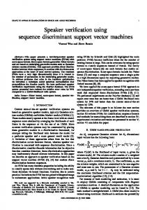
3.1 Linear SVM for linearly separable data We will start with the simplest case: linear machines trained on linearly separable data. Therefore consider the d problem of separating a set of training vectors xi∈ 3 belonging to different classes yi ∈ {-1, 1}. We wish to separate this training set with a hyperplane: w.x + b = 0
(1)
For the sake of simplicity we assume that the data space is 2 3 as on figure 3. There are actually an infinite number of hyperplanes that could partition the data into two sets (dashed lines on figure 3). According to the SRM principle, there will just be one optimal hyperplane: the hyperplane lying half-way the maximal margin (we define the margin as the sum of distances of the hyperplane to the closest training points of each class). The solid line on figure 3 represents this Optimal Separating Hyperplane, the margin in this case is d1+d2.
cost for violating the separation constraints (3). This can be done by introducing positive slack variables ξi in constraints (3), which then become: yi.(xi.w + b) ≥ 1 - ξi , ∀ i (4) If an error occurs, the corresponding ξi must exceed unity, so Σi ξi is an upper bound for the number of classification errors. Hence a logical way to assign an extra cost for errors is to change the objective function (2) to be minimized into: min { ½ ||w||² + C. (Σi ξi ) }
(5)
where C is a chosen parameter. A larger C corresponds to assigning a higher penalty to classification errors. Minimizing (5) under constraint (4) gives the Generalized Optimal Separating Hyperplane. This still remains a QPproblem.
3.3 Non-linear SVM
Figure 3: Optimal Separating Hyperplane
Note that only the closest points of each class determine the Optimal Separating Hyperplane. These points are called Support Vectors: if all other training points were removed from the set and training was repeated, the same Optimal Separating Hyperplane would be found. As only the Support vectors determine the Optimal Separating Hyperplane they are in a certain way representative for a given set of training points It has been shown [1] that the maximal margin can be 2 found by minimizing ½ ||w|| : min {½ ||w||² }
(2)
The Optimal Separating Hyperplane can thus be found by minimizing (2) under the constraint (3) that the training data is correctly separated. yi.(xi.w + b) ≥ 1 , ∀ i
(3)
This is a Quadratic Programming (QP) problem for which standard techniques (Lagrange Multipliers, Wolfe dual) can be used.
3.2 Linear SVM for non-linearly separable data The concept of the Optimal Separating Hyperplane can be generalized for the non-separable case by introducing a
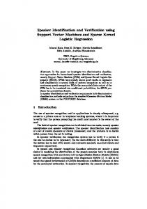
So far we used a linear separating decision surface. In the case where decision function is not a linear function of the data, the data will be mapped from the input space (i.e. space in which the data lives) into a high dimensional space (feature space) trough a non-linear transformation. In this (high dimensional) feature space, the (Generalized) Optimal Separating Hyperplane is constructed. This is illustrated on figure 4.
Optimal Separating Hyperplane in Feature Space
Feature Space Non-linear Transformation
Input Space
Figure 4: Non-linear SVM This non-linear transformation is performed in implicit way trough so-called kernel-functions. The use of implicit kernels allows reducing the dimension of the problem and overcoming the co called “dimension curse” [1]. The kernels must satisfy some constraints in order to be valid (Mercer’s Condition [2]). For binary classification following kernel are most often used: • K(xi,xj)=xIxj : linear SVM p • K(xi,xj)=(xIxj+1) : polynomial of degree p • K(xi,xj)=tanh(a.xIxj+b) and a>b: multi-layer perceptron (MLP) classifier • K(xi,xj)=exp {||xI -xj||² / σ²} : radial basis function (RBF) classifier
Note: Training an SVM usually implies a large scale QPprogramming problem [6,8] so the use of appropriate specific SVM QP-methods such as Chunking [2], Sequential Minimal • Optimization [14] are desirable to avoid problems with stability, memory size, computing time,…
4 Experimental results 4.1 Experimental setup All the tests have been carried out using the M2VTS [13] database and using the same experimental setup as described in [10]. This setup includes: • The experimental protocol used to extract impostor and client tests out of the M2VTS database. We used 111 client/3996 impostor tests for the training of the SVM and 37 client/1332 impostor tests for the testing of the performances of the SVM • A set of 3 experts: a profile and a frontal expert based upon the correlation of gray-values and a textdependant vocal expert based upon similarity measures. The performances of the individual experts I used are given in table 1. Expert
Mean Value FRR(%)
FAR(%)
TSR(%)
Vocal
29.5
0.0
85.6
Profile
11.1
30.6
79.2
Frontal
5.0
7.8
93.6
6.4%). This means that there is a considerable « fusion gain » The TER of a linear SVM is equal to the TER of the non-linear SVM. This implies that the «nature » of the data is more or less linear. The non-linear separating surface degenerates to a linear one. This illustrates the power of an SVM although the SVM is allowed to use a complex (non-linear) separating surface, it prefers a simple (linear) one in order to separate the data.
•
4.3 An extension: SVM with weighted norm So far we have discussed « classical » SVM, which are designed to separate data without any a priori knowledge. In the specific case of person verification though we do have a priori information on the data through the performances of the used experts, represented by their TSR. So it could be useful to introduce this knowledge into the SVM. This can not be done using on of the three existing parameters of a “classical” SVM (particular choice of kernel function/ parameter(s) of kernel/ parameter C for penalization of classification errors). Hence we’ll have to expand the concept of SVM to take the differences between the experts into account. A possible way to do so for a linear SVM is to use the TSR of the experts as weights for the maximization of the margin. It is indeed more useful to have a bigger margin for a (reliable) expert with high TSR than for a (less reliable) expert with lower TSR. Equation (2) shows that maximizing the margin is equivalent to minimizing the L2norm of w. The expression of the L2-norm gives (4): w =
w 12 + w 22 + ... + w n2
Table 1: Experts
We clearly see that for a “classical” SVM every expert has a component with equal contribution to the margin. If we want to attribute different weights to each component we will have to use the weighted norm ||w||g (5),
4.2 Results When using SVM to “fuse” the results of the three experts we obtain following results. As we work with a finite number of tests a 95 % confidence interval is given between square brackets. SVM-kernel Linear Poly (p=2) (p=10) RBF (σ=0.5) (σ=0.3) MLP (a=0.5,b=-1)
FRR(%) (37 tests) 2.7 [0.5,13.8] 2.7 [0.5,13.8] 2.7 [0.5,13.8] 2.7 [0.5,13.8] 2.7 [0.5,13.8] 5.4 [1.5,17.7]
FAR(%) (1332 tests) 0.0 [0.0,0.3] 0.0 [0.0,0.3] 0.0 [0.0,0.3] 0.0 [0.0,0.3] 0.1 [0.0,0.5] 0.1 [0.0,0.5]
TER(%) (1369 tests) 0.1 [0.0,0.5] 0.1 [0.0,0.5] 0.1 [0.0,0.5] 0.1 [0.0,0.5] 0.1 [0.0,0.5] 0.2 [0.1,0.6]
Table 2: Experimental results This leads to following conclusions:
•
(4)
The mean value of the TER (≅ 0.1%) is lower than the TER of the best expert (frontal expert: TER =
w = g12w12 + g22w22 + ...+ gn2wn2 g
(5)
where gi²is the weight of expert i. Which weights should we take? Because a reliable expert (i.e. with high TSR) has to have a bigger influence on the margin, the weight for the margin must be proportional to the TSR. But as the margin itself is inversely proportional to ||w|| g (2), the weights for w must be inversely proportional to the TSR (6) : 1 g i2 = (6) TSR i This formulation has the further advantage tha classical SVM-algoritms still can be used. Indeed, define G as g1 0 G= . 0
0 g2 ...
0 0 ... . 0 g n ... ...
(7)
The weigthed norm can now be written as (8) : T ||w||g = ||G.w || (8) Training a classical SVM implies the minimisation of (2) under constraint (3) : min {½ ||w||² } (9) yi.(xi.w + b) ≥ 1 , ∀ i Training a SVM with weighted norm on the other hand implies : T Min { ||G.w ||} (10) yi.(xi.w + b) ≥ 1 , ∀ i *
T
*
-1
T
Note that if we put w = G.w and x =(G .x) , the SVM with weighted norm (10) w.r.t. w and x becomes equivalent to a classical SVM (9) w.r.t. w* and x* so standard SVM techniques can be used to solve SVM with weighted norm. The TSR of the used experts are given in table 1.When using SVM with weighted norm to “fuse” the results of the three experts we obtain following results. SVM-kernel SVM Weighted Norm
FRR(%) (37 tests) 0.0 [0.0,9.4]
FAR(%) (1332 tests) 0.0 [0.0,0.3]
TER(%) (1369 tests) 0.0 [0.0,0.3]
Table 3: SVM with weighted norm The fact that we have only developed a linear SVM with weighted norm is no restriction as the nature of the data of the problem is linear anyway (see conclusions 4.2). Extension to the non-linear case implies the use of kernel functions.
5 Conclusions Table 4 gives the results of a wide range of parametric and non-parametric fusion-methods [10] carried out using the same experimental setup. This table includes the results we obtained for a linear SVM and SVM with weighted norm. Method
FRR(%) (37 tests) Multi Linear 2.7 Max. a posteriori 5.4 Logistic Regression 2.7 Quadratic Classifier 0.0 Linear Classifier 0.0 MLP 0.0 OR-voting 0.0 And Voting 8.1 Majority-voting 0.0 k-Nearest Neighbor 8.1 k-NN+Vector Quant. 0.0 Binary Decision Tree 8.1
FAR(%) (1332 tests) 0.7 0.0 0.0 2.4 3.1 0.4 7.4 0.0 3.2 0.0 0.5 0.3
TER(%) (1369 tests) 0.7 [0.4,1.3] 0.1 [0.0,0.5] 0.1 [0.0,0.5] 2.3 [1.6,3.2] 3.0 [2.2,4.0] 0.4 [0.2,0.9] 7.2 [5.9,8.7] 0.2 [0.1,0.6] 3.1 [3.1,4.2] 0.2 [0.1,0.6] 0.5 [0.2,1.0] 0.5 [0.2,1.0]
Linear SVM SVM Weighted Norm
0.0 0.0
0.1 [0.0,0.5] 0.0 [0.0,0.3]
2.7 0.0
Table 4: Comparison of different fusion-methods
This shows that: • The best result so far was obtained using a Logistic Regression model. A classical linear SVM equals this result. The fact that Logistic Regression is also a linear model confirms the earlier conclusion that the most robust solution for this particular problem is a linear one (see 4.2). • A SVM with weighted norm outperforms a classical SVM and gives the best result of all proposed methods. This gain is due to the fact that there are significant differences in the TSR of the different experts. If all TSR were the same the output of a weighted SVM would be identical to that of a classical one. • SVM (based on SRM-principle) yields better performance than a MLP (based on ERM-principle). This confirms the theoretical advantages of SRM. These results show that the use of SVM is a very performing, promising and flexible method to realize decision fusion in a multi-modal identity verification system. The interpretation of the obtained results should be not be done in an absolute way. The error percentages should be considered more as a relative comparison between different methods on a same experimental setup. An absolute interpretation of the 0.00%TER of a weighted SVM could give the impression of an error-free verification system. One should take into account though the fact that the number of tests is limited, that the tests are done in “laboratory-circumstances”, that they depend on the experts used,… A further considerable advantage of SVM in addition to other methods is the fact that very few parameters needs to be fixed or estimated. In other methods the choice of parameters is very difficult and time-consuming and demands often a lot of a priori knowledge about the training data. The choice of the few parameters of an SVM (kernel function/parameter of kernel function/penalty of misclassification) is more general and does not necessarily influence the final results in a considerable way.
References [1] Vladimir N. Vapnik . “The Nature of Statistical Learning Theory”. Springer, 1995. [2] Vladimir N. Vapnik . “Statistical Learning Theory”. Wiley Interscience, 1997. [3] Christopher J.C. Burges. “A Tutorial on Support Vector Machines for Pattern Recognition”. Bell Laboratories, Lucent Technologies. Data Mining and Knowledge Discovery, Vol. 2, Number 2, p. 121-167, 1998. [4] M.O. Stitson, J.A.E. Weston, A. Gammerman, V. Vovk, V. Vapnik. “Theory of Support Vector Machines”. Royal Holloway Technical Report CSD-TR-96-17, 1996 [5] Steve Gunn. “Support Vector Machines for Classification and regression”. University of Southampton ISIS, 1998
[6] Edgar E. Osuna, Robert Freund, Frederico Girosi. “Support Vector Machines : Training and Applications”. Massachusetts Institute of Technology, Artificial Intelligence laboratory, C.B.C.L. Paper N° 144,1997 [7] A.J. Smola. “Learning with Kernels”. GMD Berlin Ph.D Thesis, 1998 [8] R. Fernandez. “Expériences numériques avec divers méthodes d’optimisation quadratique sur le PQ associé au calcul d’une SVM”. Universit” Paris 13, Rapport Technique, 1997 [9] Souheil Ben-Yacoub. “Multi Modal Data Fusion for Person Authentication using SVM”. IDIAP-RR 9807,1998 [10] P. Verlinde. “A Contribution to Multi-Modal Identity Verification using Decision Fusion”. ENST-Paris Ph.D. Thesis, 1999. [11]G.R. Walsh. “Methods of Optimisation”. Wiley&Sons, 1985 [12]William H.Press, Brian P. Flannery, Saul A. Teukosky, William T. Vettering. “Numerical Recipies in C : the art of scientific computing”, Cambridge Universty Press, 1992 [13]ACTS, “Multi-modal verification for tele-services and security applications”, www.uk.infowin.org/ACTS/RUS/PROJECT/ac102.htm, 1995 [14]J. Platt. “Fast Training of Support Vector Machines using Sequential Minimal Optimization”, in Advances in Kernel Methods – Support vector Learning , B. Schölkopf, C. Burges, and A. Smola, eds., MIT Press, 1998.