International Conference on Computer Systems and Technologies - CompSysTech’ 2005
Using Support Vector Machine as a Binary Classifier Nikolay Stanevski, Dimiter Tsvetkov Abstract: This paper presents a relatively new and less known alternative of the classical neural network architectures – Support Vector Machines (SVM) and their usage for binary data classification. After a brief description of the Statistical Learning Theory – the framework of SVM, we explore the ways to build an error-tolerant binary classifier for linearly and non-linearly separated data. A comparison between SVM and some other neural network types is performed. To illustrate the paper, a demonstration software is provided. Key words: Support Vector Machines (SVM), Neural Networks (NN), Artificial Intelligence (AI)
INTRODUCTION A resurgence of interest in neural networks has been observed since 80s. Together with well known architectures and training algorithms, like singlelayer and multilayer perceptron, trained with backpropagation algorithm, there is a plenty of other approaches. Support Vector Machine (SVM) is among the emerging approaches here. It can be used for many AI tasks (e.g. text categorisation, image recognition, gene expression etc. [3]). The problem we will explore here is following. We have a set S of pairs (x i , yi ) ,
i = 1,2,K, N , where x i ∈ ℜ n and every vector x i is labelled to belong to any of two subclasses via yi where yi is a scalar which value can be either 1 or -1 indicating that the corresponding vector x i belongs to a particular subclass C1 or C2 . The goal of the paper is to design a SVM which performs such binary classification. BINARY CLASSIFICATION FOR LINEARLY SEPARABLE DATA, USING MAX MARGIN CLASSIFIER There are a lot of approaches to linearly separate two data classes. We can use, for example, a single or multi-layer perceptrons. Solutions of the problem (i.e. neuron weight vectors w and biases b ) are an infinite set and depend on some factors like initial weights and biases, learning algorithm and its parameters etc. The problem here is to find the only optimal margin of the separating hyperplane w T x + b = 0 , the one that provides maximum wide boundary between the classes ( w T x stands for the dot product of the vectors w and x ). This margin guaranties the lowest rate of misclassification. As mentioned above, the dataset contains two classes of data. Suppose the set S is strongly linearly separable. Then there exists uniformly separating hyperplane w T x + b = 0 and a positive κ > 0 so that w T x + b ≥ κ for x ∈ C1 and w T x + b ≤ − κ for x ∈ C2 therefore via normalizing any uniformly separating hyperplane α can be defined by the property (1) w T x + b ≥ 1 for x ∈ C1 and w T x + b ≤ −1 for x ∈ C2 . Given a separating hyperplane α which satisfies conditions (1), for the distances between α and the points x ∈ S we have wT x + b 1 , (2) dist (x, α ) = ≥ w w therefore the optimal hyperplane is the one with maximal 1 / w that guaranties an optimal margin of width 2 / w because the equality in (2) is reached at least for one point x1 ∈ C1 and at least one point x 2 ∈ C2 . Obviously maximizing that distance means minimizing following dot product
- - IIIA.14-1 - -
International Conference on Computer Systems and Technologies - CompSysTech’ 2005
1 T w w. (3) 2 On the other hand for all points we have (4) yi ( w T x i + b ) − 1 ≥ 0 . Put together, (3) and (4) represent a quadratic constrained optimization problem which can be stated as 1 minimize w T w , (5) 2 subject to yi (w T x i + b) − 1 ≥ 0 , i = 1,2,K, N . One important note here is that the target function is convex. The solution of the optimization task for convex functions is always its global minima. The problem, described by (5) is known as primal problem. This problem has its corresponding dual problem. One common way to solve it is by using of the Lagrangian function N 1 L(w, b, α) = w T w − ∑ α i yi w T x i + b − 1 , (6) 2 i =1 where α i are known as Lagrange multipliers. L(w, b, α) reaches its minima at the point which satisfies both ∂L(w, b, α) ∂L(w, b, α) = 0, = 0, (7) ∂b ∂w together with the Kuhn-Tucker conditions [2]. Applying these conditions we reduce our problem to the solution of the dual problem N 1 N N T maximize (with respect to α ) ∑ α i − ∑∑ α i α j yi y j x i x j , (8) 2 i =1 j =1 i =1
[ (
N
subject to
∑α y i =1
i
i
) ]
= 0 and α i ≥ 0 , i = 1,2,K, N .
(9)
After calculating α i we can find the weight vector w and the bias b we need by the formulas N
N
i =1
i =1
w = ∑ α i yi x i , b = − ∑ α i w T x i
N
∑α i =1
i
.
(10)
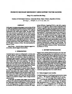
The picture below shows how our demo SVM classified linearly separable data.
Figure 1: SVM working on linearly separable data. Circles show one class, squares – the other. Support vectors are pointed out by crosses.
There are two important properties we should note here.
- - IIIA.14-2 - -
International Conference on Computer Systems and Technologies - CompSysTech’ 2005
•
Only the points x ∈ S with dist (x, α ) = 1 / w (laying on the margin hyperplanes) have
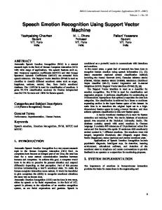
their corresponding α i nonzero. These points are so-called support vectors (hence the name Support Vector Machine). • The input patterns are always represented as a set of dot products. This will make it possible to easily switch to nonlinear SVMs as further described. SOFT MARGIN SVM The case described above is sometimes useless, because there are some factors (e.g. as a result of noise, fluctuations etc.) and it is not possible to find a hyperplane that strictly divides the data. Here, we can find an error-tolerant margin, called soft margin. To describe it, we first introduce the so-called slack variables ξ i which measure the deviation between the real and the ideal position of each point. If ξ i = 0 the point is on the right side, ξ i > 1 means wrong side, and 0 < ξ i ≤ 1 means the marginal band. Then (4) can be generalized as (11) yi (w T x i + b) ≥ 1 − ξi , i = 1,2,..., N . Now the primal problem is to minimize (with respect to w ) the following function N 1 T w w + C ∑ ξi , (12) 2 i =1 subject to the same constraints. The parameter C controls how much error-tolerant the machine is. The corresponding dual problem does not use slack variables. The only difference here is that the Lagrange multipliers should satisfy 0 ≤ α i ≤ C instead of α i ≥ 0 for each training sample (x i , y i ) . For the optimal weight and bias here we have N N ⎛ N ⎞ w = ∑ α i yi x i , b = ⎜ ∑ (C − α i )α i yi − ∑ (C − α i )α i w T x i ⎟ i =1 i =1 ⎝ i =1 ⎠ The following picture is an illustration of this case.
N
∑ (C − α )α i =1
i
i
.
(13)
Figure 2: Soft margin SVM: Filled by stars samples are misclassified by the linear soft margin
NONLINEAR BINARY CLASSIFCATION USING SVM The most exciting property of SVM is the easy way it can switch from linear to nonlinear margin. It uses Cover’s theorem [2], which states that input data, which are linearly non separable into input space I (under certain assumptions) can be mapped to another space (called feature space) F , in which data can be linearly separable. The main problem here is to find a map function Φ : I → F . Given that fact, the dot T product is now transformed as x i x j → Φ T (x i )Φ (x j ) . If there is a kernel function K which
- - IIIA.14-3 - -
International Conference on Computer Systems and Technologies - CompSysTech’ 2005
satisfies K (x i , x j ) = Φ T (x i )Φ (x j ) then the calculations will be entirely on K . Thus the problem becomes to find a linear margin into new feature space F . Then the conditions (8) can be generalized to N 1 N N (14) maximize (with respect to α ) ∑ α i − ∑∑ α i α j yi y j K (x i , x j ) , 2 i =1 j =1 i =1 N
subject to
∑α y i =1
i
i
= 0 and 0 ≤ α i ≤ C , i = 1,2,K, N .
(15)
An important issue here is how to choose kernel function. It turns out that a function can be used as a kernel if it satisfies conditions of the Mercer’s theorem [2]. Most used kernels are described below. Kernel function Description T Dot product kernel K (xi , x j ) = xi x j
(
)
K (x i , x j ) = x i x j + 1
K (x i , x j ) = e
T
− xi −x j
Polynomial kernel
p
Radial basis (Gaussian) kernel
2
2σ2
(
K (x i , x j ) = tanh k x i x j − δ T
)
Sigmoidal kernel (satisfies Mercer’s theorem only for some values (k , δ ) )
Table 1: Most used kernel functions
How can a trained SVM be used for classifying an unknown vector? It depends on the sign of the following expression N
f (x) = ∑ α i yi K (s i , x) + b ,
(16)
i =1
where N N ⎛ N ⎞ N (17) b = ⎜⎜ ∑ (C − α i )α i yi − ∑ (C − α i )α i ∑ α j y j K (x i , x j )⎟⎟ ∑ (C − α i )α i . i =1 j =1 ⎝ i =1 ⎠ i =1 In the sums above it holds α i > 0 only for the support vectors hence they play the main role during the usage phase. Nonlinear SVM is illustrated below. In the right side it is shown the shape of the separating surface (in addition zero plane is shown).
Figure 3: Nonlinear SVM: Gaussian kernel K ( x i , x j ) = e
−
xi − x j
2σ
2
2
with
σ =1
is used.
When the Gaussian kernel is used it appears a great amount of support vectors. In the example above we have N = 59 samples and N s = 29 support vectors. In the next example we use a polynomial kernel.
- - IIIA.14-4 - -
International Conference on Computer Systems and Technologies - CompSysTech’ 2005
(
)
Figure 4: Nonlinear SVM: Polynomial kernel K ( x i , x j ) = x i x j + 1 T
3/ 2
is used.
It is interesting to compare SVM with other neural network architectures. Compared to multilayer perceptron (backprop algorithm), it is seen that sigmoidal-kernel SVM is actually a perceptron with one hidden layer with N s neurons on it. Here the learning algorithm selects the optimal amount of support vectors, while for the perceptron it depends on the network designer how many hidden layer neurons will be used. In addition the perceptron learning algorithms (e.g. gradient descent) are slower than SVM learning. Another advantage is that quadratic programming always finds the global minima, while for backpropagation there is a danger to be trapped into a local minima. CONCLUSIONS AND FUTURE WORK SVM is a good alternative of the well know backpropagation neural networks. Based on quadratic optimization of convex function, this architecture can easily switch from linear to nonlinear separation, i.e. from input to feature space. This is realized by nonlinear mapping using so-called kernel functions. A topic for future work would be to explore in depth properties of different kernel functions for particular applications. The authors thank to Assoc. Prof. Svilen Stefanov for the help in the technical preparing of the examples above. REFERENCES [1] Burges, C.J.C., A tutorial on Support Vector Machines for Pattern Recognition, Data Mining and Knowledge Discovery vol.2, p. 121-167, 1998 [2] Cristianini N., J.S. Taylor, An Introduction to Support Vector Machines and Other Kernel-based Learning Methods, Cambridge University Press, 2000 [3] Haykin, S., Neural Networks – A Comprehensive Foundation, Delhi, India, 1999 ABOUT THE AUTHORS Nikolay Stoyanov Stanevski, PhD student, Military Unit 24430 – Troyan, Phone: +359 670 2 58 59, E-mail:
[email protected] Assoc.Prof. Dimiter Petkov Tsvetkov, PhD, Department of Mathematics, National Military University “Vassil Levski”, Veliko Tarnovo, Phone: +359 62 600 210, Е-mail:
[email protected]
- - IIIA.14-5 - -