Ella Atkins. â ..... distance d km in the positive YV direction. ... Satellite 2, offset by d=10 km in the baseline case, requires additional force in order to ..... S. Mehra, R. Smith, R. Beard, âMulti-spacecraft Trajectory Optimization and Control Using.
Multi-Mode Orbit Optimization for Satellite Virtual Rigid Body Formation Maintenance Ella Atkins†
Yannick Penneçot‡ Abstract
Formation flight will significantly improve space-based data collection capabilities.
Full
trajectory optimization over the spectrum of formation and orbital parameters is critical due to high fuel cost but is computationally prohibitive.
To reduce complexity, this paper presents an
approach to optimize long-term satellite formation maintenance, specifically distinguished from its assembly, where assembly is defined as the transition between launch vehicle deployment state and formation initialization.
Central-body potential fields are presumed, and optimal
solutions utilize a combination of natural drift, impulse, and low-thrust active control modes within each orbit. The formation planner is embedded within an end-to-end simulation platform that includes a high-fidelity dynamics simulator and 6-DOF controller. Formation geometry and motion are specified by a series of coordinate transforms that define a virtual rigid [or flexible] body.
A two-satellite formation applicable to the MAXIM/Pathfinder mission is optimized,
with results demonstrating the utility of the multi-mode control approach to formation flight.
1 Introduction Satellite formation flying is achieved when relative position and/or attitude constraints are imposed on a spacecraft group.
Formation flight may reduce launch costs due to smaller
satellite size/weight (nanosats), will improve fault tolerance through redundancy, and is proposed for a variety of astronomical missions requiring large-field data collection.
In Earth or
heliocentric orbits, gravitational forces require either fuel expenditure or the computation of † ‡
Assistant Professor, Aerospace Engineering Dept., University of Maryland, College Park, MD 20742 Graduate Research Assistant, Aerospace Engineering Dept. University of Maryland, College Park, MD 20742
1
clever drift orbits to meet data collection constraints despite curved-space motion. Drift orbits with correction burns are defined for missions such as LISA (Laser Interferometer Space Antenna) and EO-1 (Earth Observing One), while full-time active control is proposed for formations such as XEUS (X-ray evolving universe spectroscopy).
Natural orbit formations
exhibit limited flexibility with respect to geometry and reconfigurability.
Conversely,
continuous active satellite control allows arbitrary formation motion at potentially prohibitive fuel costs. The tradeoff between active control cost and natural orbit motion constraints suggests optimally coupling the two solutions to minimize overall fuel expended and allow arbitrary formation geometries.
This paper describes a search-based formation optimization algorithm
and evaluates the utility of a hybrid active/drift formation control strategy for rigid two-satellite orbiting formations such as the proposed MAXIM (MicroArcsecond X-ray Imaging Mission) Pathfinder (http://maxim.gsfc.nasa.gov/pathfinder.html). A general formation planner would optimize over all satellite motion from launch vehicle deployment through data acquisition.
The planner would receive the set of initial states and
constraints (e.g., geometry, pointing) as input and would output individual satellite trajectories. This problem can be divided into two dependent sub-problems as illustrated in Fig. 1: formation assembly, the computation of trajectories from initial positions (e.g., Xs1 , Xs 2 ) to arrival at the synchronized data acquisition states (e.g., Xf 1 and Xf 2 ), and formation maintenance, the specification of synchronized satellite trajectories to maintain formation shape over time. To reduce the optimization parameter search-space to a manageable size, this research addresses the maintenance sub-problem for virtual rigid body (VRB) formations in elliptical or circular orbits, solving for the combination of active and impulse maneuvers that maximize data collection with minimum formation-wide cost over a single orbit, where cost is a function of fuel use and assembled formation (data collection) time.
2
Presuming repeating elliptical orbits,
optimizing over one orbit also yields the best solution for n orbits.
Strict optimization over
maintenance is viable for long-term formations in which assembly fuel use is dwarfed by fuel required for data collection. For shorter-term formations, overall cost must be optimized. This paper begins with a discussion of related work and equations (Sections 2 and 3). The formation planner is part of an end-to-end distributed formation flight simulator outlined in Section 4.
The set of formation coordinate frames used to define VRB geometry and relative
motion throughout the simulator is also described.
Cast as a constrained optimization problem,
the planning algorithm (Section 5) receives parameter minimum and maximum boundaries and finds the best combination of these parameters where “best” is defined as least fuel consumed per second of data collection time. The current implementation utilizes Keplerian dynamics with Lambert’s solution calculations for optimizing drift orbit regions, enabling relatively fast solutions at the price of unmodeled perturbations.
Results from two-satellite formation
optimizations are presented (Section 6), with emphasis on characterizing effects of varied active control - drift region position and size.
2 Related Work This work concentrates on automated satellite formation optimization in gravity fields. The bulk of formation flight research to-date3,6,14,19 has focused on relative navigation and distributed control.
Although the formation trajectory optimization field is relatively unexplored,
several mission-specific solutions have been presented.
To minimize fuel, successful orbiting
formation designs to-date have exploited either chaser-follower arrangements along the same orbit track (e.g., EO-15 ) or natural periodic elliptical trajectories11 expressed in the Hill frame (e.g., Techsat-219,8 ).
Analytical solution for these trajectories is typically performed assuming
ideal central force motion as does this work, with recent research16 including J2 during equation linearization. Halo orbit motion7 has also been used to define natural formation geometries.
3
During flight, real-time trajectory adjustments are required to correct for unmodeled perturbations.
EO-1, the follower satellite of Landsat-7, has provided a first step toward
spacecraft autonomy during formation flight. Using the Autocon5 mission and maneuver planning software, EO-1 computes burns that re-center the satellite in the defined orbit window. This work is a crucial step toward autonomous trajectory planning but relies on manual window definition for follower satellite realignment. Formations with constraints such as the fixed inertial orientation required for MAXIM/Pathfinder are not solved with periodic orbital trajectories, and natural assembly strictly at apogee is also infeasible when data must be collected continuously for extended time periods. Trajectory generation for such complex formation geometries has typically employed optimal control techniques in a flat-space environment8 .
Trajectories for flat-space formations are also
planned using a genetic algorithm (GA) with multi-parameter cost function10 .
Researchers3,4
have utilized an exhaustive search approach to optimal satellite rotation in flat space with cost function terms including total consumed fuel and fuel equalization among spacecraft.
Flat-space
collision avoidance is addressed as a guidance algorithm with separation constraints17 .
This
paper describes orbit optimization for arbitrary formation geometries in gravity fields, requiring use of active control to maintain formation geometry but relaxing those constraints during “drift” periods in which the formation is not maintained.
Solutions do not yet account for collisions,
non-Keplerian perturbation effects, or cost elements beyond fuel usage and data collection time. This method emphasizes generality in formation definition and search parameters, and results illustrate the benefits of distinct active/drift modes.
3 Equations For this work, optimization assumes perfect central-force motion. with constant inertial offset from a natural orbit.
4
Consider a satellite
This satellite must have exactly the same
acceleration as the point it follows on the natural orbit, and the overall force vector on the satellite must accommodate this motion. Each such satellite in a VRB is submitted to the force
r r supplied by its thrusters Fcont and to the force Fsat from the Earth’s gravitational field as given by the Law of Universal Gravitation: r µ r Fsat = M sat ⋅ r 3 r r
(1)
r where Msat is satellite mass and r is the vector from the central body to the satellite.
r The acceleration a T of the target point on the natural orbit to be followed by the satellite can be found by calculating the gravity field at that point: r µ r a T = r 3 rT rT
(2)
r r where rT is the distance from the center of the Earth to the target point. The vector r can be r r expressed as a function of rT and offset vector ∆r :
r r r r = rT + ∆r
(3)
r r Force Fcont the thruster must apply for the satellite to match a T is then given by:
(
r r r µ ⋅ M sat r r r µ Fcont = aT ⋅ M sat − Fsat = rT − M sat ⋅ r r 3 ⋅ rT + ∆r 3 rT rT + ∆r
)
(4)
Eqn. (4) provides a simple Keplerian approximation to force required for formations with constant offset between the satellite and natural orbit target point. This result can be extended to formations with relative motion among member satellites as shown in Eqn. (5).
In this case,
r satellite acceleration is a T plus the acceleration required in flat space to follow the predefined r r relative velocity profile. Force Fcont when ∆r varies with time is then:
5
(
)
r r µ ⋅ M sat r r r µ Fcont = rT − M sat ⋅ r r 3 ⋅ rT + ∆r + M sat ⋅ ∆&r& 3 rT rT + ∆r
(5)
r Once Fcont is computed for each time step the total ∆v needed to maintain the satellite on its nonnatural orbit is found by integrating over each active control region:
∆v = ∫
t final
tinitial
r Fcont M sat
dt
(6)
The above equation pair is used to compute fuel cost during active control. Lambert’s algorithm2 computes initial and final impulse maneuvers for each satellite to match formation position and velocity for the next active control pass following drift. The adopted algorithm was based on the simulation written for the Voyager 2 mission.
4 Formation Specification and Simulation The ideal formation simulation environment would allow a scientist to issue commands such as “maintain formation geometry/shape S1 for minimum time T1 given orbital constraints O1 and precision (position/attitude) α 1 ”. The simulator would then: •
Find a trajectory for each formation satellite that achieves all science goals and minimizes cost (e.g., fuel use).
•
Apply navigation and control strategies that maintain accuracy α 1 in 6 DOF.
•
Simulate the formation using realistic, high-accuracy dynamics during tracking of the trajectories computed by the planner or specified by the user.
•
Display simulation results and compare ideal and actual results at all levels.
The simulator must incorporate a variety of gravity fields, including geosynchronous and lowEarth orbits, Lagrange points, and heliocentric orbits, with either inertial or LVLH (Local Vertical Local Horizontal) attitude reference. Developed as a collaborative effort15 , Fig. 2 shows
6
the complete simulation platform that meets the above requirements and includes the formation planner/optimizer described in this paper.
For speed and to model the actual computer cluster
present for ground/satellite operations, a distributed computer network was constructed where each satellite is simulated by a dedicated computer (Sat-i, i=1,…,5) and another simulates the ground station (Groundcon). An additional computer (Satcon) maintains a global reference time and acts as a dynamics propagator. Groundcon simulates the trajectory computation functions of a ground control station. Through a GUI (Fig. 3), the user specifies formation fixed geometric and orbit constraints. The user also specifies search parameter minimum, maximum, and stepsize. The planner, running on Groundcon, identifies the minimum-cost set, which are converted into a waypoint plan and broadcast to the simulated satellites through local high-speed Ethernet. Five computers, Sat-1 through Sat-5, simulate up to five formation satellites. The controller generates thrust levels from the present state trajectory
(X )given d
( X ) of
by the trajectory synthesis module.
the satellite and from the desired
The next state of the satellite is
computed from the thrust levels output by the controller and from the gravity fields output by Satcon. The state of all satellites is then forwarded to Groundcon to allow real-time formation viewing via the Satellite Tool Kit (STK), as shown in Fig. 4. Formation Coordinate Frames To precisely define geometry and coordinated motion of multiple bodies in threedimensional space, a set of reference frames are utilized throughout all simulation modules. Fig. 5 illustrates frame attachments for a three-satellite virtual rigid body (VRB) example.
Inertial
frame I is the global reference frame, then "target" coordinate frame T is tracked by the entire formation. T frame orbital parameters specify its translational motion with attitude defined to match either inertial or Earth-pointing (LVLH) coordinates.
The actual position of the overall
formation is frame V, defined relative to the T frame. The T frame is associated with a natural
7
orbit, which may be aligned, offset, or time-varying with respect to V. The separation of V and T frames allows the system to represent multi-body tracking operations such as rendezvous and docking. It also allows arbitrary formation pointing and motion relative to the T frame. Coordinate frame set Dk is defined to specify individual satellite positions and attitudes relative to the V frame. Dk frame positions specify geometry (shape). If all Dk positions are constant with respect to V, a virtual rigid body (VRB) is defined. Otherwise, geometry changes and a virtual flexible body (VFB) with individual satellite motions are specified. Within the planner, V and T frame attitudes are currently referenced directly to inertial or LVLH coordinates, a simplification to be extended in future work.
5 Formation Optimization The formation planner must identify the optimal set of orbital T frame and geometric V, Dk frame parameters to define the assembled (or “actively-maintained”) VRB or VFB. Additionally, the planner must optimize the size and location of orbital regions in which the formation is actively assembled versus freely drifting.
Because this research concentrates solely
on formation maintenance, the planner may select a snapshot anywhere along the formation orbit to initialize execution of each plan.
Elliptical orbits are presumed and allow formation
maintenance to extend over multiple orbits. During execution, the formation may be repeatedly assembled following drift segments.
Because the formation is maintained throughout the active
region, it is assumed the total time summed over all active regions (per orbit) is equal to total data acquisition time per orbit. To reduce complexity, the planner makes a number of simplifying assumptions. As discussed previously, orbits are presumed Keplerian and elliptical, requiring the central body to be a point mass much greater than the satellites. All perturbations are also ignored. Guidance, navigation, and control algorithms and sensors/actuators are presumed sufficient to track
8
specified trajectories, and thruster limitations such as saturation, vibration, and plume impingement are ignored. Recall that the planner is but one component of the overall simulation architecture; the controller and dynamic simulator model thrust through duty cycling of impulse engines, a technique that has been shown 15 to provide micrometer position accuracy. A novel feature of the formation planner is optimization over multiple operational modes, including active control, impulsive thrust (∆v), and drift (no thrust). Associated mode switching may be viewed as the hybrid automaton illustrated in Fig. 6.
Consider two distinct control
modes: drift and 6-DOF active trajectory following. An impulse (∆v) may be imparted to each satellite during mode transition to initialize entry velocity conditions. When switching from active to drift, this impulse set (one per satellite) initializes transfer orbits that assemble the formation at the end of drift.
When switching from drift to active control, the impulse set
matches satellite velocities to those of the V frame for VRB data collection. Impulse maneuvers are idealized as instantaneous velocity changes enabling their modeling as transitions rather than states. Relaxing this assumption yields progressively complex automata13 . Parameter Search-Space Optimization occurs over position and size of active vs. drift control regions as well as T, V, and Dk frame parameters that specify formation motion. Fig. 7 lilustrates the primary search parameters (for one active control region) utilized in this work.
An active region width, λ,
describes the angle over which the VRB is assembled for data acquisition. If λ=0, the formation continuously drifts with no controller intervention. When λ=2π, the VRB is maintained throughout the orbit. Large λ yield long observation times at the cost of potentially significant fuel usage. As described previously, impulsive maneuvers are used to switch between active and drift modes. No impulse is required for the extrema (0, 2π) since no mode switches occur. In other cases, mode switch impulse magnitudes are dependent on satellite positions and velocities
9
relative to the reference orbit. The center of the active control region, ξ, is defined as the angle from the perigee of the T orbit to the center of the active region. When ξ=0, the controlled segment is centered on perigee, and when ξ=π, the active region is centered on apogee. The time of drift Tdrift is defined as the time during which the satellites drift from the end of active control to the beginning of the next data acquisition sequence. The search for Tdrift is performed around the time it would take for the T frame to traverse its corresponding drift orbit segment.
Formation orbit is specified by the standard parameters (a, e, i, ω, Ω, ν) for the T
frame1,2, with V and Dk frame motion defined relative to T. The semi-major axis a is feasible so long as the orbit is higher than the atmosphere and sufficiently small to be reached during assembly. From the maintenance perspective, the larger a, the less fuel will be expended. Based on Eq. (4), the force (magnitude) Fcont required to maintain a satellite of mass Msat away from its natural orbit can be estimated to first order as: Fcont ≈− M sat
µ r 1+ 2.∆r
(7)
where r is instantaneous T frame altitude (computed from a, e, ω, ν) and ∆r is the altitude difference between the satellite and r. For maintenance, where assembly costs due to boosting orbit altitudes are ignored, semi-major axis a is set to its maximum value to minimize r. T frame eccentricity e must be sufficiently small that altitude at perigee is greater than the atmospheric altitude below which the satellite should not drop. Intuitively, maintenance cost (fuel) should decrease as satellite altitude increases, suggesting that high-eccentricity formations with active regions near apogee may minimize fuel usage. The target frame argument of perigee ω allows the planner to select the best alignment between target frame semi-major axis and observation target, as shown in Fig. 7. The optimal choice depends on formation geometry, specifically seeking conditions in which formation satellites are as close as possible to the
10
reference orbit during active and impulse maneuvers. Because formations continue through multiple orbits and may be initialized at any orbit location, ν is not a factor for optimization. The remaining elements, i and Ω, are also not explored since assembly and perturbation terms are ignored. For a VRB, individual satellite position/orientation (Dk frame) is fixed relative to V. However, the planner may minimize cost by positioning V relative to T. Generally, three offsets (Xv, Yv, Zv) are optimized except for in-plane formations in which only (Xv, Yv) are examined. To summarize, the planner optimizes over parameter set P1 ={λ, ξ, Tdrift, a, e, ω, Xv, Yv, Zv}.
The user provides minimum, maximum, and step-size values for each parameter and may
additionally specify n ≥ 0 non-overlapping active regions per orbit, in which case Pn ={(λ1 , ξ 1 , Tdrift,1), ..., (λ n , ξ n , Tdrift,n), a, e, ω, Xv, Yv, Zv) is optimized. Algorithm and Waypoint Plan Specification To guarantee convergence on a globally optimal solution and examine individual parameter effects on optimality, an exhaustive search strategy was adopted for planning. Total cost per orbit for all Pn value combinations are computed, with the overall minimum returned as the solution.
The user may define constant values for any Pfixed ⊆ Pn with remaining search
parameters Popt={Pi | Pi∈Pn , Pi∉Pfixed}. Each Pi∈Popt is optimized over user-specified [Pmin,i, Pmax,i] with stepsize ∆Pi, yielding nv i = (Pmax,i - Pmin,i)/ ∆Pi possible values. Through this flexible interface, any parameter subset can be explored, facilitating rapid evaluation of cost for fixed parameter sets Pfixed=Pn as well as the study of single or dual parameter effects on overall cost. For m search parameters Pi ∈Popt with nv i possible values, the computational complexity m for exhaustive search is O ∏ nvi . i=1
With n active control regions, a full VRB optimization
(Popt=Pn , Pfixed=∅) is performed over m=(3n+6) parameters.
Search complexity substantially
limits feasible parameter and value sets given even the fastest processors.
11
For example, one
active control region (n=1) yields nine search parameters. With Popt=Pn and each Pi discretized to nv i=20 values, computational complexity is O(209 ) or O(1011 ). For reasonable (one week or less) completion times and parameter value sets nv i sufficient to avoid function aliasing, expansion to n>1 regions is greatly facilitated with a populated fixed parameter set Pfixed. To find the overall cost for each parameter value combination, the total cost for active control and impulsive maneuvers are summed over exactly one maintenance orbit.
The
parameter value set Pn plus fixed VRB Dk frame definitions uniquely define satellite positions and velocities associated with the active control region.
To compute active control cost, the
planner integrates Eqn. (7) over the active region. Drift orbits and associated entry/exit impulse pair for each satellite is computed via Lambert’s algorithm2 as discussed previously.
All
optimization software is written in C, and numerical results for several fixed parameter sets were verified with independent Matlab software.
Individual ∆v values required for active control
force balance were also verified by hand. The optimal Pn are encoded as a waypoint plan to be transmitted to the trajectory synthesis module on each simulated satellite.
Each waypoint plan W={w 1 , w2 , …, ws} is
composed of s sequential segments wi over one orbit and may be repeated for multi-orbit simulations.
Each segment wi={T i, WV i, WDk,i, qref} defines the associated target frame Ti, V
frame waypoint WVi, and [optional VFB] Dk frame waypoint set WDk,i={WDSat-1,i, …, WDSat-k,i} for the k-satellite formation. An additional mode flag qref specifies whether formation attitude is inertial or LVLH.
V frame waypoints WVi={t i, cm i, v i(t i), ωi(t i)} are composed of waypoint
activation/arrival time t i, control mode cm i, velocity vector v i(t i), and angular velocity vector ωi(t i). Dk frame waypoints have analogous content. Note that arrival time t i is given with respect to simulation initialization rather than astronomical time, and control mode specifies whether the formation is to be actively controlled, drifting, or experiencing ∆v from time t i to t i+1 . A linear
12
interpolator synthesizes reference trajectory values between waypoints, and true astronomical time is defined separately for the simulator 12 . Optimality criteria The planner optimizes using a cost function based on parameter value set Pn : Cost = f (Pn ) = f (λ1 ,ξ 1 , Tdrift,1 ,..., λn , ξ n , Tdrift, n , aT , eT , ω T , X V , YV , ZV )
(8)
For the k-spacecraft formation flight problem, the following factors are considered: •
Minimize overall fuel expenditure during active control
•
Minimize overall fuel expenditure during impulsive maneuvers
•
Maintain uniform fuel distribution across the k satellites10
•
Maximize data acquisition time, assumed equal to active control (assembled) time
Cost function f would typically utilize weighting factors to assign relative importance.
As a
simple trade between fuel use and observation time, the following cost was adopted: Cost =
∆vcont + ∆vimp
(9)
t cont
∆v cont is the continuous ∆v per orbit summed over all k satellites, ∆v imp is the impulsive ∆v per orbit summed over all k satellites, and t cont is the total active control (data acquisition) time per orbit. Note that other cost functions can easily be accommodated by the planner; such additions would be based on user preference and mission requirements.
6 Two-Satellite Case Study Consider an inertial-pointing, planar, two-satellite formation. Defined as a VRB, the two satellites have fixed relative position, with one satellite at the V frame origin and the other a distance d km in the positive YV direction. Both satellites have the same mass (1000 kg) and thruster performance (idealized low-magnitude Isp = 2000 sec).
13
This example is feasible for
missions such as far-field interferometry (Fig. 8) or MAXIM/Pathfinder (formations rotated 90° in Fig. 8) and illustrates the impact of active and drift modes on cost. Secondarily, effects of altering T frame parameters are studied. V frame offset is ignored due to its minimal effect on cost for this formation1 . To strictly examine the effects of active control region size and width, a scenario set was constructed with one active region (n=1) and all parameters Pn fixed except Popt = {λ1 , ξ 1 , Tdrift,1}. Shown in Fig. 8, three cases (a-c) were optimized with manually-altered orbit eccentricity e and argument of perigee ω.
T frame altitude a is 50000 km and the orbit is equatorial (i,Ω=0). As
defined, satellite 1 is aligned with T thus follows a zero-thrust natural orbit during active control. Satellite 2, offset by d=10 km in the baseline case, requires additional force in order to maintain the VRB. For both satellites, impulses computed by Lambert’s solution are applied at the beginning and end of active control to synchronize final positions and velocities. Note that plots illustrate cost as a function of λ1 and ξ 1 . Tdrift,1 is optimized but not studied separately. Two cost functions were examined: observation (9).
fuel use per orbit (∆v imp +∆v cont) and fuel use per second of
The latter was primarily studied due to observation time necessity for any
mission. Fig. 9 shows fuel required per orbit (∆v in m/sec) for Case a summed over both satellites for the two impulse maneuvers. When ξ ±
λ = 0 or π, the satellites are as close as possible to 2
their natural orbit at the time of impulse application, yielding local cost minima. local maxima occur when ξ ± at impulse initiation.
Conversely,
λ = π/2 or 3π/2 since Sat-2 is maximally far from its natural orbit 2
When λ=2π, no impulses are required since the formation is constantly
maintained. Fig. 10 shows active control fuel required as a function of ξ and λ. As expected, when λ is zero, there is no active control thus no fuel required. Fuel cost varies almost linearly in
14
λ with variations due to average distance of Sat-2 from the T frame orbit during active control. When λ=0 or 2π, ξ has no influence on cost since the whole orbit is either completely controlled or uncontrolled. control costs.
Total cost in fuel use (Fig. 11) was found by summing impulsive and active Due to the dominance in the active control cost, the minimum exists for λ=0,
indicating minimum cost when the formation is uncontrolled.
However, this minimum has zero
observation time, suggesting migration to the fuel per observation second cost function. Fig. 12 shows active control fuel per observation second cost. Two minima (λ=0.01, ξ=0 or π) occur because the VRB is maintained when both satellites are close to the natural orbit, and maxima occur when Sat-2 is actively controlled far from the natural orbit. When λ>π most of the active region is far from ξ; and cost is mitigated by average distance of each satellite from T. For example, when ξ=0 and λ=3π/2, the formation is maintained primarily where the satellites are far from T.
This explains the inversion from minimum to maximum as λ increases until
approaching 2π for which ξ is no factor. Fig. 13 shows total cost in fuel per observation second for Case a (circular orbit). In this example, optimal conditions exist when λ=2π, indicating that the best strategy is to control the formation throughout the orbit with no impulsive maneuvers. Cases b and c (Fig. 8) have T frame orbits with e=0.5 but perpendicular arguments of perigee (ω=0 and π/2, respectively). Fig. 14 shows impulse ∆v required for Case b. Behavior resembles the circular orbit example except minima migrate closer to apogee and maxima cluster closer to perigee, where gravitational forces are strongest. Fig. 15 shows Case c total impulse. For small λ, the satellites drift most of the orbit. When the formation is centered at perigee (ξ=0), Sat-2 is far from the T frame orbit and close to Earth, yielding maximum fuel use with small λ. Although of much less magnitude due to increased distance from the central body, when ξ approaches apogee, satellite altitude again moves away from T, resulting in a local maximum with small λ. Fig. 15 also shows a maximum at (ξ=π, λ=3π/2). This occurs because the inner 15
satellite is closer to the Earth (higher angular speed) and the outer one is farther (lower angular speed), and they must achieve the opposite condition following a π/2 drift near perigee. This condition may be mediated by swapping satellite positions (rotating the VRB by π), but such a swap will not significantly affect minima, the values in which we are interested.
Active control
cost (∆v/sec) for Cases b and c both have maxima near perigee (ξ=0) and minima near apogee (ξ=π). The perigee maxima dominate plots of active control cost thus are not shown. Total costs (∆v/sec) for Cases b and c are shown in Figs. 16 and 17, respectively, with significantly highest cost solutions found at apogee for Case c and near but not at apogee for Case b due to the tradeoff between Sat-2 proximity to T frame at perigee versus proximity to Earth. Both cases have absolute minimum at apogee (ξ=π), but the minimum cost for Case b (best case) is significantly lower than that for Case c due to differences in Sat-2 offset from T. Table 1 provides a summary of cost (in ∆v per observation second) for all examples studied, with the “best” result (Case b) provided first as the baseline. Again consider Cases a – c to assess the utility of multi-mode active/drift orbits. The minimum cost (4.93e-5 m/s2 ) for the circular orbit case (a) occurs at λ=2π, and the circular orbit is the overall optimum when fulltime active control is required due to the high cost of formation maintenance near perigee. The minimum cost (1.89e-5 m/s2 ) for the best-case elliptical orbit (b) occurs at (λ=0.01, ξ=π) with observation time 1.3 hours per orbit, while Case c minimum cost (2.94e-5 m/s2 ) is found at (λ=2.14, ξ=π) with large active region width due to the maximal Sat-2 offset from T at apogee for this case. This data indicates that the elliptical orbit with ω=0 yields minimum overall cost per observation second. However, this result also provides less continuous observation time per orbit, especially compared to orbital period, indicating the satellite must be deployed for a longer total time to obtain a given amount of data.
16
Table 1: Two-satellite Inertial-Pointing Optimal Result Summary. # Case
active
d
a
regions
(km)
(km)
Obs.
Active
ω
ξ
λ
Time
Time
Cost
(rad)
(rad)
(rad)
(hrs)
(%)
(m/sec2 )
e
1 (b)
1
10
50000 0.5 0
π
0.01
0.13
0.418
1.89E-5
2 (c)
1
10
50000 0.5 π /2
π
2.14
20.6
66.7
2.88E-5
3 (a)
1
10
50000 0.0 N/A
N/A
2π
30.9
100
4.93E-5
4
2
10
50000 0.5 0
(2.8,3.2)
(0.01,0.61)
7.66
24.8
2.38E-5
5
2
10
50000 0.5 π /2
(2.0,3.2)
(0.01,2.21)
21.0
68.1
3.02E-5
6
1
10000 50000 0.5 0
π
0.14
1.79
5.78
1.88E-2
7
1
10
10000 0.5 0
π
0.02
0.023 0.831
2.36E-3
8
1
10
50000 0.5 0
π
0.20
2.55
8.24
1.91E-5
9
1
10
50000 0.5 0
π
2.14
20.6
66.7
3.62E-5
The remaining Table 1 cases (4-9) illustrate effects of additional parameters on cost. Again, optimization was over λ and ξ with other parameters fixed. Cases 4 and 5 show the optimal result for ω=0, π/2, respectively, when two non-zero, non-overlapping active control regions are present. For case 4, the optimal solution clusters two relatively small active regions around apogee, attempting to capture the baseline (Case b) result of one region centered at apogee. Case 5 similarly attempts to capture the Case c result, suggesting that one active region at apogee is the best solution for this example regardless of VRB orientation (ω value).
Cases 6
and 7 vary inter-satellite distance (d) and T frame altitude (a), verifying that the optimal solution is a small active region around apogee at different cost. Cases 8 and 9 illustrate the sensitivity of cost to changes in active control region width.
17
In Case 8, λ is increased from the optimal
baseline value of 0.01 to 0.2, yielding only a 1% increase in cost. In case 9, λ is set to 2.14 with ω=0 for comparison to the optimal result for ω=π/2. The corresponding cost of 3.62e-5 m/sec2 is nearly twice the optimal baseline cost (λ=0.01) and 25% greater than Case c with ω=π/2. The primary result from this study is that multi-mode active/drift operation over a highlyelliptic orbit can provide the ability to accommodate extended assembled observation times while significantly reducing cost relative to fully-active non-natural orbits. Argument of perigee ω also affects cost and choice of active region width, as illustrated by Case b vs. c. Fig. 18, computed by fixing ω at a series of values then optimizing over λ and ξ, details the effects of ω on cost, confirming that b and c are best and worst-cases, respectively.
Optimal active region
width λ increases to include regions where Sat-2 is close to T, and impulsive thrust is also applied at these regions. For this example, minimum cost increases by ~52% as a function of ω, but is always significantly lower than the circular orbit, fully active case. Typical VRBs collect data from multiple targets, requiring reorientation to align instrumentation.
VRB (V frame)
reorientation relative to T can be equivalently viewed as a change in ω, given the “maintenance” assumption that the formation can be reassembled for each orbit after drift. Further computation is required to sequence observations such that reorientation costs are minimized.
7 Future Work The coordinate representation and simulation architecture described in this paper are general to arbitrary formation geometries and motions (VRB and VFB).
However, for search efficiency,
the planner optimizes only long-term formation maintenance assuming central-force motion. Research is currently underway to refine solutions via a two-stage search in which Keplerian dynamics plus J2 harmonics are used to identify the optimal parameter neighborhoods followed by a local search using the full dynamic simulation propagated about complete orbits. A multi-
18
stage search process is also under consideration to automatically refine parameter step sizes and range limits based on gross identification of expected low-fuel regions. Attitude maneuver cost is currently ignored due to the presumption of multiple thrusters along all axes, a significant simplification when high ∆v maneuvers require main engine firing. Plans are now constructed for a k-satellite rigid formation. Although each plan is optimal with respect to its model, consideration of the following will also be important: •
Coupled formation assembly and maintenance to produce globally-optimal plans
•
Swapping satellite VRB positions during drift segments to potentially reduce overall cost when satellites are interchangeable
•
Optimizing V-frame motion (rather than static offset) relative to T, enabling minimumcost maneuvers such as rendezvous/docking
•
Enabling Virtual Flexible Body (VFB) formations by optimizing Dk frame trajectories relative to V
8 Conclusions Science data collection considerations may require complex formation geometries and motions difficult or impossible to achieve with strictly natural orbits.
This research studies the
combination of active control and drift orbit segments to minimize fuel usage (∆v) per data collection second for virtual rigid body (VRB) formation maintenance. by a hierarchical group of coordinate frames.
Formations are defined
A target (T) frame defines formation reference
orbit, a vehicle (V) frame describes formation motion with respect to T, and individual satellite frames (Dk ) define motion with respect to V.
An exhaustive search algorithm optimizes over
orbital parameters as well as active control region position (ξ) and width (λ) to identify
19
minimum-cost formation maintenance solutions.
The planner is embedded in an end-to-end
distributed simulation architecture. An in-plane inertially-pointing two-satellite formation is studied. achieved
for
maximum-altitude,
maximum-eccentricity
reference
orbit
Minimum cost is with
formation
maintained near apogee. Active region width λ depends on formation geometry as well as orbit eccentricity and argument of perigee. Even the simple two-satellite example studied in this work illustrates the benefit of switching between active and drift control modes during formation maintenance. surprising.
The presence of active control near apogee and drift near perigee was not However, the variance in active control region width due to the tradeoff between
distance from central body and satellite proximity to the natural orbit was less predictable. Although perturbations were ignored for this research, the high-fidelity dynamics propagator will provide a near-term means both to study errors in predicted cost and to provide a future means for refining optimal solutions. This research describes a method for planning satellite trajectories when orbiting formation geometries and motion are dictated solely by science rather than fit into natural orbit constraints.
Although potentially expensive, such solutions must be considered as
missions become more ambitious and sophisticated.
9 Acknowledgement The authors would like to thank University of Maryland collaborators Dr. Robert Sanner, Will Miller, and Suneel Sheikh for their work on formation representation, control, and simulation. This research was partially supported under NASA grant NAG59961.
10 References 1
E. Atkins and Y. Penneçot, “Autonomous Satellite Formation Assembly and Reconfiguration with Gravity Fields,” in Proc. IEEE Aerospace Conference, Big Sky, Montana, March 2002. 20
2
R. H. Battin, An Introduction to the Mathematics and Methods of Astrodynamics, AIAA Education Series, 1987.
3
R. Beard and F. Hadaegh, “Finite Thrust Control for Satellite Formation Flying with State Constraints”, in Proc. of the American Control Conference, San Diego, June 1999.
4
R. Beard and F. Hadaegh, “Fuel Optimized Rotation for Satellite Formation in Free Space”, in Proc. of the American Control Conference, San Diego, June 1999.
5
D. E. Conkey, G. T. Dell, S. M. Good, “EO-1 formation Flying Using Autocon™”, IEEE, 2000.
6
D. Folta, “A 3-D Method for Autonomously Controlling Multiple Spacecraft Orbits”, IEEE, 1998.
7
F. Hsiao and D.J. Scheeres, “The Dynamics of Formation Flight about a Stable Trajectory,” in Proc. 2002 Space Flight Mechanics Meeting, San Antonio, Texas, January 2002.
8
E. M.-C. Kong, Spacecraft Formation Flight Exploiting Potential Fields, Ph.D. thesis, MIT, Cambridge, MA, February 2002.
9
M. Martin and M. Stallard, Distributed Satellite Missions and Technologies – The TechSat21 Program, AIAA Paper No. 99-4479, 1999.
10
S. Mehra, R. Smith, R. Beard, “Multi-spacecraft Trajectory Optimization and Control Using Genetic Algorithm Techniques”, IEEE, 2000.
11
M. Milam, N. Petit, R. Murray, “Constrained Trajectory Generation for Micro-Satellite Formation Flying”, Proc. of AIAA Guidance, Navigation and Control Conference and Exhibit, Montreal, August 2001.
12
W. Miller, “Development and Analysis of a Satellite Formation Flying Path Planner and Simulator”, Space Systems Lab Technical Report, University of Maryland, 2002.
21
13
Y. Penneçot, E. Atkins, R. Sanner, "Intelligent Spacecraft Formation Management and Path Planning," Proc.
AIAA Aerospace Sciences Conference, Reno, NV, January 2002 (AIAA
2002-1072). 14
M. de Queiroz, V. Kapila, Q. Yan, “Adaptive Nonlinear Control of Multiple Spacecraft Formation Flying”, Journal of Guidance, Control and Dynamics, Vol. 23, No 3, May-June 2000.
15
R. M. Sanner and S. Sheikh, “Distributed Testbed for the Simulation of Satellite Formation Flight”, Space Systems Laboratory Technical Report, University of Maryland, 2003.
16
R. J. Sedwick, E. M. C. Kong, D. W. Miller, “Mitigation of Differential Perturbations in Clusters of Formation Flying Satellites,” Journal of the Astronautical Sciences, Vol. 47, Nos. 2 and 4, July – December 1999.
17
G. Singh and F. Hadaegh, “Collision Avoidance Guidance for Formation-Flying Applications”, Proc. of AIAA Guidance, Navigation and Control Conference and Exhibit, Montreal, August 2001.
18
D. A. Vallado, Fundamental of Astrodynamics and Applications, Space Technologies Series, 1997.
19
P. K. C. Wang, F. Hadaegh, K. Lau, “Synchronized Formation Rotation and Attitude Control of Multiple Free-Flying Spacecraft,” Journal of Guidance, Control, and Dynamics, Vol. 22, No. 1, Jan – Feb 1999.
22
X f 1, t f 1
X S1 , t S1 X S 2 , tS 2 Initial orbit Assembly / Transfer orbit
X f 2, tf 2
Maintenance trajectory
Figure 1 – Satellite formation assembly and maintenance.
23
Satellite States
STK™ 3-D VO Simulation Time
STK/ Connect
GUI Mission Parameters
Simulation Ephemerides
Satcon
Plans
Trajectory Synthesis
Control Laws
Satellite Dynamics
State
Sat-1
Waypoint Planner Groundcon
Thrust Levels
Trajectory Synthesis
Control Laws
Thrust Levels
Satellite Dynamics
State
Sat-5
Figure 2 – Formation flight simulation architecture.
24
Figure 3 – Formation Parameter Specification GUI.
25
Figure 4 - STK™ 3-D Formation Visualization.
26
D 3 frame T-frame
I-frame
V-frame
D 2 frame D1 frame
Figure 5 - Formation frame attachment.
27
∆V
∆V
Active Control Mode
Drift Mode
∆V
Figure 6 – Hybrid Automaton Plan Representation.
28
∆V
Inertial Observation Target YI Controlled Segment
Reference Orbit
λ
ω
θ
XI
ξ
Figure 7 – Formation parameter definition with distinct active and drift orbit regions.
29
Target
a. Circular (e=0)
b. e=0.5, ω=0
c. e=0.5, ω=π/2
Figure 8 – Inertial-pointing two-satellite interferometry T frame orbit configurations.
30
∆v (m/s)
λ (deg)
ξ (deg)
Figure 9 – Impulsive maneuver ∆v per orbit for Case a (circular orbit).
31
∆v (m/s)
λ (deg)
ξ (deg)
Figure 10 – Active control ∆v per orbit for Case a.
32
∆v (m/s)
λ (deg)
ξ (deg)
Figure 11 – Total ∆v per orbit for Case a.
33
∆v/sec (m/s2 )
λ (deg) ξ (deg) Figure 12 – Active control ∆v required per observation second for Case a.
34
∆v/sec (m/s2 )
λ (deg)
ξ (deg)
Figure 13 – Total ∆v per observation second for Case a.
35
∆v (m/s)
λ (deg)
ξ (deg)
Figure 14 – Impulsive maneuver ∆v for Case b (e=0.5, ω=0).
36
∆v (m/s)
λ (deg)
ξ (deg)
Figure 15 – Impulsive maneuver ∆v required for Case c (e=0.5, ω=90º).
37
∆v/sec (m/s2 )
λ (deg) ξ (deg) Figure 16 – Total ∆v cost per observation second for Case b (e=0.5, ω=0).
38
∆v/sec (m/s2 )
λ (deg) ξ (deg) Figure 17 – Total ∆v cost per observation second for Case c (e=0.5, ω=90º).
39
∆v/sec (m/s2 )
Figure 18 – Optimal cost per observation second as a function of ω.
40