Multi-objective Active Control Policy Design for Commensurate and Incommensurate Fractional Order Chaotic Financial Systems Indranil Pana, Saptarshi Dasb and Shantanu Dasc
a) Energy, Environment, Modelling and Minerals (E2M2) Research Section, Department of Earth Science and Engineering, Imperial College London, Exhibition Road, London SW7 2AZ, United Kingdom. b) Communications, Signal Processing and Control (CSPC) Group, School of Electronics and Computer Science, University of Southampton, Southampton SO17 1BJ, United Kingdom. c) Reactor Control Division, Bhabha Atomic Research Centre, Mumbai-400085, India. Authors’ Emails:
[email protected],
[email protected] (I. Pan)
[email protected],
[email protected] (S. Das)
[email protected] (Sh. Das)
Abstract: In this paper, an active control policy design for a fractional order (FO) financial system is attempted, considering multiple conflicting objectives. An active control template as a nonlinear state feedback mechanism is developed and the controller gains are chosen within a multi-objective optimization (MOO) framework to satisfy the conditions of asymptotic stability, derived analytically. The MOO gives a set of solutions on the Pareto optimal front for the multiple conflicting objectives that are considered. It is shown that there is a trade-off between the multiple design objectives and a better performance in one objective can only be obtained at the cost of performance deterioration in the other objectives. The multi-objective controller design has been compared using three different MOO techniques viz. Non Dominated Sorting Genetic Algorithm-II (NSGA-II), epsilon variable Multi-Objective Genetic Algorithm (ev-MOGA), and Multi Objective Evolutionary Algorithm with Decomposition (MOEA/D). The robustness of the same control policy designed with the nominal system settings have been investigated also for gradual decrease in the commensurate and incommensurate fractional orders of the financial system. Keywords: chaos control; chaotic financial system; commensurate and incommensurate order system; fractional order nonlinear systems; multi-objective active control 1. Introduction Investigations into chaotic dynamics of physical systems have revealed a variety of different fields where this is found and financial systems have been documented to show significant chaotic behaviour [1]. On contrary, fractional calculus driven modelling techniques especially fractional Brownian motion have received huge focus as a potential tool 1
to describe the dynamical behaviour of the stochastic variations in financial time series [2]. Data driven modelling of financial systems has been shown to obey a power law characteristics i.e. the Fourier transform spectra decays as a power law with respect to frequency [3], [4]. It has been shown by Meerschaert and Scalas [5] that in finance, the relation between random variables like log-returns and waiting time can be suitably modelled using FO partial differential equations. FO noise characteristics have also been used to identify the economic periods of crisis from financial time series in [6]. Effect of parameter switching on such FO chaotic financial systems have been studied by Danca et al. [7]. Other perspectives of financial modelling e.g. FO volatility model has also been developed [8] for empirical market data. The concept of FO financial model has been extended to variable order financial systems [9] where the fractional orders changes over time. These studies show that sudden big fluctuations in financial time series give rise to the power law characteristics and has a close relation with fractional calculus. A realistic FO macroeconomic model was estimated using the national economic data of UK, Canada and Australia in the studies by Skovranek et al. [10]. Similar nonlinear model parameter estimation has been proposed using least squares to model macroeconomic data of USA [11] and interest rate change in Japan [12]. Studies have also found that the presence of time delays in such financial systems modifies the chaotic behaviour of the system where one policy change take some time to modify the overall system’s dynamics [13]. It has also been found that complex financial systems show both stochastic and deterministic dynamics where the first branch has emerged to model typical behaviours like non-stationarity, non-Gaussianity, randomness and long range dependence (or power law characteristics) of such systems as discussed earlier. The other branch has emerged while analysing significant nonlinear dynamical behaviour like chaos, bifurcation [14] and hyperchaos [15] in such large scale financial systems. There have been attempts to investigate chaotic dynamics in financial time series using delay embedding based phase space reconstruction, Lyapunov exponent estimation by parametric and non-parametric methods [16], recurrence plots [17] etc. Apart from the practical data or time series based studies, continuous time [14] as well as discrete time models [18] have been proposed to model chaotic dynamics of financial systems. Thus the co-existence of chaotic and FO characteristics are inherent in financial systems which motivates the study of an active control policy for such systems. These chaotic dynamics are undesirable and must be supressed to reduce financial risks and improve the performance of the economy [17]. Classically there exists two broad methods for chaos control, viz. the OGY (Ott-Greborgi-Yorke) method of intermittent control and the continuous control method [19], [20]. FO economical or financial system [21] has been controlled or synchronized using several approaches e.g. sliding mode [22], time delayed feedback [23], linear control [24], lag projective synchronization [25], Lyapunov linearization and stability condition [26] etc. In [27], the control of the uncertain FO financial system has been attempted using adaptive sliding mode control. However in all the above cases, chaos control has been done from a stability point of view but the control performance has not been taken into consideration. Other computational intelligence based techniques 2
which use intelligent algorithms for chaos control [28], [29] or synchronisation [30] take the performance measure of fast synchronisation or control in the formulation of the objective function itself. However, the drawback of this type of design methodology is that guaranteed analytical stability is not enforced in the process and thus the scheme may not work for initial conditions other than the one used in the simulation. Also only a single objective has been considered as a performance measure in the designs reported in [29], [30]. In a practical design problem there exists multiple trade-offs among a set of conflicting objectives. Therefore a design methodology must take these challenges into account and come up with optimal solutions which meet these objectives to a sufficient level. In other words there is a requirement for multi-objective optimisation methods to be applied to these problems to arrive at efficient designs. Multi objective synchronisation for chaotic systems has been recently investigated in [31] where the coupling strengths between the two chaotic systems are optimised using an evolutionary multi-objective optimisation. However, in this case, the analytical stability is not included within the optimisation algorithm. Thus using the methodology proposed in [31], it might happen that for different values of initial conditions, the chaotic systems do not synchronise. This is because, the synchronisation has only been achieved in a mean squared sense and guaranteed analytical stability of the error dynamical system is not enforced. In the present paper, the concept of multi-objective synchronisation of chaotic systems in [31] has been extended to the case of chaos control. Unlike the approach in [31], the analytical stability conditions for chaos control have been incorporated within the optimisation algorithm itself. This ensures stability of the optimised solutions in all cases, even when considering different initial conditions. To the best of our knowledge, the present paper can be considered as the first attempt for active control policy design for commensurate and incommensurate FO chaotic systems in a multi-objective framework with guaranteed analytical stability considerations. The rest of the paper is organised as follows. Section 2 outlines the preliminary background of fractional calculus along with the numerical methods for simulating FO chaotic systems. Section 3 introduces the FO financial system and proposes the mathematical underpinnings of the active control strategy. Section 4 highlights the need for multi-objective optimisation in chaos control and describes the NSGA-II, ev-MOGA and MOEA/D algorithms briefly as multi-objective optimisers. Section 5 illustrates the results and discussions. The paper ends with the conclusions in Section 6 followed by the references. 2. Mathematical preliminaries 2.1. Basics of fractional calculus Fractional calculus is an extension of the integer order successive differentiation and integration for any arbitrary real order. The fundamental operator representing the noninteger order differentiation or integration is given by a Dtα in (1), where α ∈ ℝ is the order of the differ-integration and a and t are the bounds of the operation.
3
α α d dt , α > 0 α α =0 a Dt = 1, t ( dτ )α , α < 0 ∫a
(1)
There are three main definitions of fractional calculus viz. the Grünwald-Letnikov (GL), Riemann-Liouville (RL) and Caputo. Other definitions like that of Weyl, Fourier, Cauchy, Abel and Nishimoto also exist. In the FO systems and control related literatures mostly the Caputo’s fractional differentiation formula is referred. This typical definition of fractional derivative is generally used to derive FO transfer function models from FO ordinary differential equations with zero initial conditions. According to Caputo’s definition, the α th order derivative of a function f ( t ) with respect to time is given by (2) α a Dt f ( t ) =
m t D f (t ) 1 dτ , α ∈ ℝ + , m ∈ ℤ + , m − 1 ≤ α < m α +1− m ∫ a Γ ( m − α ) (t −τ )
(2)
t
where, Γ (α ) = ∫ e−t t α −1dt is the Euler’s Gamma function. This definition is used in the present 0
paper for realizing the fractional integro-differential operators of the chaotic system. The Caputo definition of fractional derivative is advantageous for control related applications over the Riemann-Liouville definition, since it only needs initial conditions for integer order derivatives and not initial conditions of fractional derivatives. The Laplace transform of the Caputo fractional derivative is given by (3) [32]. m −1
∞
L 0 Dtα f ( t ) = ∫ e − st 0 Dtα f ( t ) dt = sα F ( s ) − ∑ sα − k −1 f m ( 0 ), m − 1 ≤ α < m 0
(3)
k =0
For zero initial condition, the Laplace transform of the three definitions boils down to the same expression sα F ( s ) which are extensively used in many modern control applications. Also, continuous or discrete time rational approximation techniques for the FO differintegrator s ±α are often employed for simulation [33]. 2.2. Numerical method for simulating fractional order chaotic systems Chaotic coupled differential equations can be numerically simulated using the power series expansion method, Adams-Bashford-Moulton predictor corrector method [34], continued fraction expansion (CFE) method [35] etc. As has been shown in Petras [32], the chaotic FO differential equations in (4) can be written in the form of a set of integral equations as in (7) and band limited rational approximations can be used for realizing the fractional differentials. This method is adopted in the present paper for simulating the FO chaotic system.
4
For a set of coupled fractional differential equations of the form (4), 0 0 0
Dtq1 x ( t ) = f ( x ( t ) , y ( t ) , z ( t ) )
Dtq 2 y ( t ) = g ( x ( t ) , y ( t ) , z ( t ) )
(4)
Dtq 3 z ( t ) = h ( x ( t ) , y ( t ) , z ( t ) )
considering the fact that the fractional differ-integrals are linear operators, i.e. a
Dtα ( λ f ( t ) + µ g ( t ) ) = λ a Dtα f ( t ) + µ a Dtα g ( t )
(5)
and the fact that the FO derivative commutes with the integer order derivative, i.e.
n dn α α d f (t ) α +n D f ( t ) ) = a Dt = a Dt f ( t ) n (a t n dt dt
(6)
Equation (4) can also be written in the form of integral equations as (7). x (t ) = 0 D
1− q1 t
t ∫ f ( x ( t ) , y ( t ) , z ( t ) ) dt 0
t y ( t ) = 0 Dt1− q2 ∫ g ( x ( t ) , y ( t ) , z ( t ) ) dt 0 t z ( t ) = 0 Dt1− q3 ∫ h ( x ( t ) , y ( t ) , z ( t ) ) dt 0
(7)
With the implementation of this transformation a Matlab/Simulink based environment is capable of simulating the FO chaotic systems as shown by Petras [32]. Each value of the FO differ-integrals {1 − q1 ,1 − q2 ,1 − q3 } is rationalized with Oustaloup’s 5th order rational approximation [36]. The FO differ-integrals are basically infinite dimensional linear filters. However, band-limited realisations of FO elements are necessary for simulation. In the present simulation study each FO element has been rationalised with Oustaloup’s recursive filter [36] given by the equations (8) and (9). If it be assumed that the expected fitting range or frequency range of controller operation is (ωb , ωh ) , then the higher order filter which approximates the FO element sα can be written as (8) [37]. N
G f ( s ) = sα = K ∏
k =− N
s + ωk′ s + ωk
(8)
where the poles, zeros, and gain of the filter can be evaluated as:
ωk = ωb (ωh ωb )
1 k + N + (1+α ) 2 2 N +1
, ωk′ = ωb (ωh ωb )
5
1 k + N + (1−α ) 2 2 N +1
, K = ωhα
(9)
In equations (8) and (9), α is the order of the differ-integration and ( 2 N + 1) is the order of the filter. The present study considers a 5th order Oustaloup’s rational approximation for
{
}
the FO elements within the frequency range ω ∈ 10−2 ,102 rad/s [36], [37]. 3. System description and theoretical formulation The FO chaotic financial dynamical system [21] is given by (10). d q1 x = z + ( y − a) x dt d q2 y = 1 − by − x 2 dt d q3 z = − x − cz dt
(10)
Figure 1: Phase portrait and state trajectories of the commensurate (q1=q2=q3=q=0.9) FO financial system.
The state variables x , y , z represent respectively the interest rate, the investment demand and the price index of a financial system. The first state variable (x) which is the interest rate can be influenced by the surplus between investment and savings along with structural adjustments from the prices. The second state variable (y) is in proportion to the rate of investment and an inversion with the cost of investment and interest rate. The third state variable (z) depends on the contradiction between supply and demand in the market and also gets influenced by the inflation rates [14]. The three constant coefficients {a, b, c} represent the savings amount, the cost per investment and the elasticity of demand of commercial markets respectively. Figure 1 and Figure 2 show the variation in the three state variables i.e. interest rate, investment demand and price index with time (in days) 6
[10] for the commensurate and incommensurate FO financial system respectively. All the three time series for both the systems exhibit erratic fluctuations, leading to a chaotic motion in the respective phase space diagrams. The second state variable (investment demand) shows more rapid fluctuation than the other two states indicating towards high spectral power in high frequency operation. Further details of the fractional financial system and its control are reported in Pan et al. [29]. Although stochastic modelling of financial systems exists in the literatures, for effective control policy development, the chaotic deterministic model of financial system is more popular.
Figure 2: Phase portrait and state trajectories of the incommensurate (q1=0.9, q2=0.95, q3=0.8) FO financial system.
For active control of the system described by (10), three active control functions
u1 ( t ) , u2 ( t ) , u3 ( t ) are considered to be applied in each of the three states of the system in (10) to yield the following set of equations. d q1 x = z + ( y − a ) x + u1 ( t ) dt d q2 y = 1 − by − x 2 + u2 ( t ) dt d q3 z = − x − cz + u3 ( t ) dt
(11)
The nonlinear active state-feedback control functions are chosen as (12)-(14) in order to make the closed loop control system linear.
u1 ( t ) = V1 ( t ) − xy
7
(12)
u2 ( t ) = V2 ( t ) − 1 + x 2
(13)
u3 ( t ) = V3 ( t )
(14)
The terms Vi ( t ) ∀ i ∈{1, 2,3} , are linear functions of the three system state variables { x, y, z} . Using equations (12),(13) and (14) in equation (11), we get (15). d q1 x = z − ax + V1 ( t ) dt d q2 y = −by + V2 ( t ) dt d q3 z = − x − cz + V3 ( t ) dt
(15)
The active control terms Vi ( t ) ∀ i ∈{1, 2,3} can be represented by (16) where the constants mij ∈ ℝ, ∀ i, j ∈ {1, 2,3} . V1 m11 V = m 2 21 V3 m31
m12 m22 m32
m13 x m23 y m33 z
(16)
Thus (15) and (16) can be clubbed together to obtain (17). x x − a + m11 D y = P y = m21 z z −1 + m31 q
m12 −b + m22 m32
1 + m13 x m23 y −c + m33 z
(17)
where q = [ q1 , q2 , q3 ] ∈ ( 0, 2 ) . T
The presence of squared and cross-product terms of the state variables in the active control inputs in (12)-(14) can be viewed as a nonlinear state feedback control design for the commensurate and incommensurate FO systems. The nonlinear control inputs makes the closed loop system linear to facilitate the established analytical stabilization schemes [32] for commensurate and incommensurate FO linear systems since such analytical stability design for the nonlinear counterpart is more involved and difficult to design. The elements of the matrix in (16) are real. Hence it might be diagonalised to produce an equivalent control action where each of the control signals is a function of its own state only and not the other states. This would remove the number of couplings and reduce the complicacies in the design process. The number of elements would have been chosen as three instead of nine and this would reduce the burden of the optimisation algorithm. However, in many cases, the eigen-values obtained as a result of such diagonalisation might be complex 8
conjugates and thus physical realisation of such state-feedback controllers with complex gains will be infeasible. Hence, all the nine components are chosen using optimization in (16) instead of choosing only the diagonals in the present approach. Another aspect of the control action that can be deduced from equations (12), (13), (14) is that, when the individual states become zero due to the application of the control action, i.e. x = y = z = 0 , then u2 becomes
( −1) and u1 and u3
becomes zero.
Now, in order to ensure asymptotic stability of system (17), the constants mij must be chosen such that the eigen-values ( λk ) of matrix P satisfy the following condition, known as Matignon’s theorem [38]. arg ( eig ( P ) ) = arg ( λk ) >
qπ ,0 qπ which signifies stable but slower operation of the system, compared to what can be achieved within a MOO framework. The reason for obtaining a dominated solution using the direct pole assignment technique compared to the Pareto solutions (in terms of control performance) is that the pole assignment scheme results in all hyper-damped and ultra-damped roots [33] leading to sluggish system operation and increase in the control effort. Unlike the commensurate FO system, in the incommensurate FO system stabilization problem, precise pole assignment becomes difficult due to the inherent higher order polynomial equation solving step. Although one can assign the eigen-values of the matrix P analytically, but manipulating the number and location of all the system roots for the characteristic equation which are distributed in different higher Riemann sheets for any arbitrary choice of incommensurate FO is still an open problem. Moreover, there would be only one solution by the direct pole-assignment approach for commensurate order system, as opposed to multiple solutions for the case of incommensurate FO system. As depicted in Figure 6, for incommensurate system also the direct pole assignment approach leads to a dominated solution, compared to what can be achieved by an MOO approach.
5.4. Discussions It is also important to mention that FO controllers have been traditionally used for enhancing the robust stability properties of linear control systems. However, for nonlinear chaotic systems extension of the robust stability properties are expected to be more complex and have not been investigated yet, to the best of our knowledge, in the fractional calculus community itself. Moreover, the proposed control strategy does not use the concept of FO controller, rather it uses nonlinear state feedback control of FO systems. Although for both the commensurate and incommensurate order systems, the active control scheme designed under the nominal system parameters faithfully suppresses chaotic oscillations with gradual decrease in fractional orders and also passes the stability checking condition but during the controller design phase such a variation has not been considered. Therefore, although the same controller works well to stabilize different FO chaotic systems, this should not be confused with robust stability where the stability of all possible inter-mediate solutions are theoretically guaranteed and has been investigated for linear FO systems only in the past.
6. Conclusions In this paper, an active control policy is derived for a FO chaotic financial system. The proposed method gives guaranteed stability, which is derived analytically for both the commensurate and incommensurate FO financial system. The active control functions are 21
then chosen using three multi-objective evolutionary algorithms to satisfy two conflicting time domain performance objectives of fast settling to the equilibrium point and small amount of controller effort requirement. The comparison of three MOOs show that the NSGA-II yields the largest Pareto front over ev-MOGA and MOEA/D but a better nondominated (although shorter) Pareto front could be achieved using MOEA/D. It is shown that the two design objectives cannot be simultaneously minimised using one particular controller. There exists a range of controllers on the Pareto front which satisfies one criterion better at the cost of performance deterioration in the other criterion. The designer can therefore choose a particular controller from these set of non-dominated solutions according to his specific problem requirements. The superiority of the proposed technique over the direct pole assignment approach [41] has also been highlighted. The effect of decreasing the fractional orders in the two type of systems (with the median solution of the controllers on the Pareto front) have been found to stabilize the chaotic systems and also pass the stability checking conditions Future work can be directed towards the multi-objective chaos control in the presence of uncertainty, noise etc. and extend the concept for robust stabilization scheme design for nonlinear chaotic systems. References [1] T. Puu, Attractors, bifurcations, & chaos: Nonlinear phenomena in economics. Springer, 2003. [2]
S. Rostek, Option pricing in fractional Brownian markets, vol. 622. Springer, 2009.
[3]
J. Tenreiro Machado, F. B. Duarte, and G. M. Duarte, “Power law analysis of financial index dynamics,” Discrete Dynamics in Nature and Society, vol. 2012, p. Article ID 120518, 2012.
[4]
F. B. Duarte, J. Tenreiro Machado, and G. Monteiro Duarte, “Dynamics of the Dow Jones and the NASDAQ stock indexes,” Nonlinear Dynamics, vol. 61, no. 4, pp. 691– 705, 2010.
[5]
M. M. Meerschaert and E. Scalas, “Coupled continuous time random walks in finance,” Physica A: Statistical Mechanics and its Applications, vol. 370, no. 1, pp. 114–118, 2006.
[6]
J. T. Machado, G. M. Duarte, and F. B. Duarte, “Identifying economic periods and crisis with the multidimensional scaling,” Nonlinear Dynamics, vol. 63, no. 4, pp. 611– 622, 2011.
[7]
M.-F. Danca, R. Garrappa, W. K. Tang, and G. Chen, “Sustaining stable dynamics of a fractional-order chaotic financial system by parameter switching,” Computers & Mathematics with Applications, vol. 66, no. 5, pp. 702–716, 2013.
[8]
R. V. Mendes, “A fractional calculus interpretation of the fractional volatility model,” Nonlinear Dynamics, vol. 55, no. 4, pp. 395–399, 2009.
22
[9]
Y. Xu and Z. He, “Synchronization of variable-order fractional financial system via active control method,” Central European Journal of Physics, vol. 11, no. 6, pp. 824– 835, 2013.
[10] T. Skovránek, I. Podlubny, and I. Petrás, “Modeling of the national economies in statespace: A fractional calculus approach,” Economic Modelling, vol. 29, no. 4, pp. 1322– 1327, 2012. [11] Z. Hu and W. Chen, “Modeling of macroeconomics by a novel discrete nonlinear fractional dynamical system,” Discrete Dynamics in Nature and Society, vol. 2013, p. Article ID 275134, 2013. [12] Y. Yue, L. He, and G. Liu, “Modeling and application of a new nonlinear fractional financial model,” Journal of Applied Mathematics, vol. 2013, p. Article ID 325050, 2013. [13] Z. Wang, X. Huang, and G. Shi, “Analysis of nonlinear dynamics and chaos in a fractional order financial system with time delay,” Computers & Mathematics with Applications, vol. 62, no. 3, pp. 1531–1539, 2011. [14] Q. Gao and J. Ma, “Chaos and Hopf bifurcation of a finance system,” Nonlinear Dynamics, vol. 58, no. 1–2, pp. 209–216, 2009. [15] H. Yu, G. Cai, and Y. Li, “Dynamic analysis and control of a new hyperchaotic finance system,” Nonlinear Dynamics, vol. 67, no. 3, pp. 2171–2182, 2012. [16] D. Guegan, “Chaos in economics and finance,” Annual Reviews in Control, vol. 33, no. 1, pp. 89–93, 2009. [17] J. Holyst, M. Zebrowska, and K. Urbanowicz, “Observations of deterministic chaos in financial time series by recurrence plots, can one control chaotic economy?,” The European Physical Journal B-Condensed Matter and Complex Systems, vol. 20, no. 4, pp. 531–535, 2001. [18] W. A. Brock and C. H. Hommes, “Heterogeneous beliefs and routes to chaos in a simple asset pricing model,” Journal of Economic Dynamics and Control, vol. 22, no. 8–9, pp. 1235–1274, 1998. [19] J. M. González-Miranda, Synchronization and control of chaos: an introduction for scientists and engineers. Imperial College Press, 2004. [20] H. Zhang, D. Liu, and Z. Wang, Controlling chaos: suppression, synchronization and chaotification. Springer, 2009. [21] W.-C. Chen, “Nonlinear dynamics and chaos in a fractional-order financial system,” Chaos, Solitons & Fractals, vol. 36, no. 5, pp. 1305–1314, 2008. [22] S. Dadras and H. R. Momeni, “Control of a fractional-order economical system via sliding mode,” Physica A: Statistical Mechanics and its Applications, vol. 389, no. 12,
23
pp. 2434–2442, 2010. [23] W.-C. Chen, “Dynamics and control of a financial system with time-delayed feedbacks,” Chaos, Solitons & Fractals, vol. 37, no. 4, pp. 1198–1207, 2008. [24] L. Chen, Y. Chai, and R. Wu, “Control and synchronization of fractional-order financial system based on linear control,” Discrete Dynamics in Nature and Society, vol. 2011, 2011. [25] G. Cai, P. Hu, and Y. Li, “Modified function lag projective synchronization of a financial hyperchaotic system,” Nonlinear Dynamics, vol. 69, no. 3, pp. 1457–1464, 2012. [26] M. S. Abd-Elouahab, N.-E. Hamri, and J. Wang, “Chaos control of a fractional-order financial system,” Mathematical Problems in Engineering, vol. 2010, p. Article ID 270646, 2010. [27] Z. Wang, X. Huang, and H. Shen, “Control of an uncertain fractional order economic system via adaptive sliding mode,” Neurocomputing, vol. 83, pp. 83–88, 2012. [28] W.-D. Chang, “PID control for chaotic synchronization using particle swarm optimization,” Chaos, Solitons & Fractals, vol. 39, no. 2, pp. 910–917, 2009. [29] I. Pan, A. Korre, S. Das, and S. Durucan, “Chaos suppression in a fractional order financial system using intelligent regrouping PSO based fractional fuzzy control policy in the presence of fractional Gaussian noise,” Nonlinear Dynamics, vol. 70, no. 4, pp. 2445–2461, 2012. [30] S. Das, I. Pan, S. Das, and A. Gupta, “Master-slave chaos synchronization via optimal fractional order PIλDµ controller with bacterial foraging algorithm,” Nonlinear Dynamics, vol. 69, no. 4, pp. 2193–2206, 2012. [31] Y. Tang, Z. Wang, W. Wong, J. Kurths, and J. Fang, “Multiobjective synchronization of coupled systems,” Chaos: An Interdisciplinary Journal of Nonlinear Science, vol. 21, no. 2, p. 025114, 2011. [32] I. Petras, Fractional-order nonlinear systems: modeling, analysis and simulation. Springer, 2011. [33] S. Das, Functional fractional calculus. Springer, 2011. [34] K. Diethelm, N. J. Ford, and A. D. Freed, “A predictor-corrector approach for the numerical solution of fractional differential equations,” Nonlinear Dynamics, vol. 29, no. 1–4, pp. 3–22, 2002. [35] Y. Q. Chen, I. Petras, and D. Xue, “Fractional order control-a tutorial,” in American Control Conference, 2009. ACC’09., 2009, pp. 1397–1411. [36] A. Oustaloup, F. Levron, B. Mathieu, and F. M. Nanot, “Frequency-band complex noninteger differentiator: characterization and synthesis,” Circuits and Systems I: 24
Fundamental Theory and Applications, IEEE Transactions on, vol. 47, no. 1, pp. 25–39, 2000. [37] Y. Chen, “Oustaloup-recursive-approximation for fractional order differentiators,” 2003. [Online]. Available: http://www.mathworks.co.uk/matlabcentral/fileexchange/3802-oustaloup-recursiveapproximation-for-fractional-order-differentiators. [38] D. Matignon, “Stability properties for generalized fractional differential systems,” in ESAIM: proceedings, vol. 5, 1998, pp. 145–158. [39] W. Deng, C. Li, and J. Lü, “Stability analysis of linear fractional differential system with multiple time delays,” Nonlinear Dynamics, vol. 48, no. 4, pp. 409–416, 2007. [40] M. S. Tavazoei and M. Haeri, “Chaotic attractors in incommensurate fractional order systems,” Physica D: Nonlinear Phenomena, vol. 237, no. 20, pp. 2628–2637, 2008. [41] S. Bhalekar and V. Daftardar-Gejji, “Synchronization of different fractional order chaotic systems using active control,” Communications in Nonlinear Science and Numerical Simulation, vol. 15, no. 11, pp. 3536–3546, 2010. [42] S. Das, S. Mukherjee, S. Das, I. Pan, and A. Gupta, “Continuous order identification of PHWR models under step-back for the design of hyper-damped power tracking controller with enhanced reactor safety,” Nuclear Engineering and Design, vol. 257, pp. 109–127, 2013. [43] H. M. Hochman and J. D. Rodgers, “Pareto optimal redistribution,” The American Economic Review, pp. 542–557, 1969. [44] A. Herreros, E. Baeyens, and J. R. Perán, “Design of PID-type controllers using multiobjective genetic algorithms,” ISA Transactions, vol. 41, no. 4, pp. 457–472, 2002. [45] I. Pan and S. Das, “Chaotic multi-objective optimization based design of fractional order PIλDµ controller in AVR system,” International Journal of Electrical Power & Energy Systems, vol. 43, no. 1, pp. 393–407, 2012. [46] G. Reynoso-Meza, S. Garcia-Nieto, J. Sanchis, and F. X. Blasco, “Controller tuning by means of multi-objective optimization algorithms: A global tuning framework,” Control Systems Technology, IEEE Transactions on, vol. 21, no. 2, pp. 445–458, 2013. [47] K. Deb, A. Pratap, S. Agarwal, and T. Meyarivan, “A fast and elitist multiobjective genetic algorithm: NSGA-II,” Evolutionary Computation, IEEE Transactions on, vol. 6, no. 2, pp. 182–197, 2002. [48] M. T. Jensen, “Reducing the run-time complexity of multiobjective EAs: The NSGA-II and other algorithms,” Evolutionary Computation, IEEE Transactions on, vol. 7, no. 5, pp. 503–515, 2003. [49] M. Laumanns, L. Thiele, K. Deb, and E. Zitzler, “Combining convergence and diversity in evolutionary multiobjective optimization,” Evolutionary Computation, vol. 10, no. 3, 25
pp. 263–282, 2002. [50] K. Deb, M. Mohan, and S. Mishra, “Evaluating the ε-domination based multi-objective evolutionary algorithm for a quick computation of Pareto-optimal solutions,” Evolutionary Computation, vol. 13, no. 4, pp. 501–525, 2005. [51] M. Martinez-Iranzo, J. M. Herrero, J. Sanchis, X. Blasco, and S. Garcia-Nieto, “Applied Pareto multi-objective optimization by stochastic solvers,” Engineering Applications of Artificial Intelligence, vol. 22, no. 3, pp. 455–465, 2009. [52] J. Herrero, M. Martinez, J. Sanchis, and X. Blasco, “Well-Distributed Pareto Front by Using the ε-MOGA Evolutionary Algorithm,” in Computational and Ambient Intelligence, Springer, 2007, pp. 292–299. [53] Q. Zhang and H. Li, “MOEA/D: A multiobjective evolutionary algorithm based on decomposition,” Evolutionary Computation, IEEE Transactions on, vol. 11, no. 6, pp. 712–731, 2007. [54] E. Zitzler and L. Thiele, “Multiobjective optimization using evolutionary algorithms—a comparative case study,” in Parallel Problem Solving from Nature—PPSN V, 1998, pp. 292–301. [55] E. Zitzler and L. Thiele, “Multiobjective evolutionary algorithms: a comparative case study and the strength Pareto approach,” Evolutionary Computation, IEEE Transactions on, vol. 3, no. 4, pp. 257–271, 1999.
26