Multi-Objective Differential Evolution (MODE) Algorithm for Multi-Objective Optimization: Parametric Study on Benchmark Test Problems
B.V. Babu* and Ashish M Gujarathi Chemical Engineering Department Birla Institute of Technology and Science (BITS), Pilani-333 031 (Rajasthan), India
Abstract: Multi-Objective Differential Evolution (MODE), a multi-population, multiobjective optimization approach using Differential Evolution (DE) has been successfully applied to selected real world problems. This algorithm is equipped with non-dominated population selection combined with basic DE algorithm. In this study, the MODE algorithm is further applied on six different Test problems with/without constraints and extensive simulation runs are carried out for parametric study. Pareto optimal solutions are obtained for each test problems. The Pareto fronts are compared on the basis of various values of key MODE parameters. This work resulted in identifying the sensitivity of various key parameters of the MODE algorithm applied on the hard test problems.
Key Words: Multi-objective optimization, Multi-Objective Differential Evolution (MODE), Pareto optimal front, Evolutionary computation, Population based search algorithms. _____________________________________________________
*Corresponding Author: Dean-EHD & Professor-Chemical Engineering Department, BITS, Pilani Tel.: +91-1596-245073 Ext. 259/212; Fax: +91-1596-244183 E-mail:
[email protected] URL: http://discovery.bits-pilani.ac.in/discipline/chemical/BVb
1. INTRODUCTION Most realistic optimization problems, particularly those in engineering design, require the simultaneous optimization of more than one objective function. Some examples are listed in Table-1: Table-1: Applications of Multi-objective optimization in Engineering Design.
Application
Objectives
Complex test problems [8, 9]
Car Purchase [33]
Simultaneous maximization and minimization of several objectives in complex test problems Low total investment and high yield of product. High Fuel Efficiency, low payload, and low weight. Low cost and high comfort
A good sunroof design in a car [33]
Low noise and high ventilation.
Automobile Design [33]
High crash resistance for safety and low weight for fuel economy. Low total mass and high stiffness.
Chemical Plant Design [33] Aircraft Design [33]
Bridge Construction [33] Supply Chain Management [8], [37]
Minimum Manufacturing Cost, Total Operating Cost, Transportation cost and Maximum Revenue/Profit. Wiped-Film Poly-Ethylene Terephthalate Minimization of acid end group (PET) Reactor [22] concentration and vinyl end group concentration Adiabatic Styrene reactor [23] Maximization of productivity and yield
In the applications listed in Table 1 and in many other cases, different solutions may produce trade-offs (conflicting scenario) among different objectives. A solution that is extreme with respect to one objective requires a compromise in other objectives. Hence, some trade-off between the criteria is needed to ensure a satisfactory design.
Because of a lack of suitable solution methodologies, a Multi-objective optimization problem (MOOP) has been mostly formulated and solved as a single objective optimization problem in the past by keeping one of the objectives as main objective and making other objectives as constraints. Traditionally, there are several methods available in the literature for solving MOOP problems [31]. These methods follow preferencebased approach, where a relative preference vector is used to scalarize multiple objectives. Since classical search and optimization methods use a point-by-point approach, where One solution in each of the iterations is modified to a different solution; the outcome of using classical method is a single optimized solution. However, Evolutionary Algorithms (EAs) can find multiple optimal solutions in a single simulation run due to their population based search approach. In this paper, MODE, a simple and fast EA is applied on six different Test problems. As Differential Evolution is found to give better results than Genetic Algorithms (GA) for single objective optimization [18, 19, 20, 11, 24, 13], we tried to extend the application of DE to MOOP problems. In our previous work [22, 23], it was observed that results obtained by MODE and NSGA were exactly matching in terms of optimum objective function values. Though both NSGA and MODE follow the same Pareto optimal front, MODE is found to perform better in terms of convergence and diversity of the Pareto Optimal front with chosen parameter values. In this work, an attempt has been made to explore the performance and robustness of MODE algorithm by further applying it on six well known Test problems with various possible parameter values.
2. DIFFERENTIAL EVOLUTION Differential Evolution [37] is an improved version of GA [32] for faster optimization. Unlike simple GA, that uses binary coding for representing problem parameters, DE is a simple yet powerful population based, direct search algorithm for globally optimizing functions with real valued parameters. Among the DE’s advantages are its simple structure, ease of use, speed and robustness. Price and Storn [37] gave the working principle of DE with single strategy. Later on, they suggested ten different strategies of DE [39]. A strategy that works out to be the best for a given problem may not work well when applied for a different problem. Also, the strategy and key parameters to be adopted for a problem are to be determined by trial and error. Pseudo code of DE for solving single objective optimization is discussed in [22]. The crucial idea behind DE is a scheme for generating trial parameter vectors. Basically, DE adds a weighted difference between two population vectors to a third vector. The key parameters of control in DE are: NP, CR, and the F- the weight applied to random differential. Price and Storn [39] have given simple rules for choosing key parameters of DE for any given application. Babu et al. [24] proposed a new concept called ‘nested DE’ to automate the choice of DE key parameters. In addition, some new strategies have been proposed and successfully applied to the optimization of extraction process [14]. DE has been successfully applied in various fields. Some of the successful applications of DE include: digital filter design [40], batch fermentation process [41, 18], estimation of heat transfer parameters in trickle bed reactor [10], dynamic Optimization of a Continuous Polymer Reactor using a Modified Differential Evolution [34], optimization of Low Pressure Chemical Vapor Deposition Reactors Using Hybrid Differential
Evolution [35], optimal design of heat exchangers [19, 20], synthesis and optimization of heat integrated distillation system [17], optimization of an alkylation reaction [7], optimization of non-linear functions [12], optimization of thermal cracker operation [11], global optimization of MINLP problems [13], optimization of water pumping systems [15], optimization of biomass pyrolysis [6], etc. Many engineering applications using various evolutionary algorithms have been reported in the literature [1, 2, 3, 4, 5, 8, 9, 16, 21, 29, 36] etc.
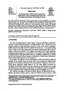
3. MULTI-OBJECTIVE DIFFERENTIAL EVOLUTION (MODE) Multi-Objective Differential Evolution (MODE) is a multi-population, multi-objective DE approach. The algorithm can be summarized as follows: An initial population is generated at random. All dominated solutions are removed from the population using the non-dominated sorting approach [31]. The remaining non-dominated solutions are retained for recombination. Three parents are selected at random. A child is generated from the three parents and is placed into the population if it dominated the first selected parent; otherwise a new selection process takes place. The schematic representation of MODE algorithm using DE approach is presented in Fig. 1. The general pseudo-code for MODE is reported in our earlier work [22, 23].
Initialize Population
Calculate Cost of all objective Functions Carry out Non-dominated Sorting and Pass corresponding variables as population to DE Generations
Target Vector
Xi
Xa
Xb
+
Xc
-
F F(Xa - Xb) Noisy ′ Random Xc = Xc + F(Xa - Xb) Vector Xt
CR Crossover
Trial Vector for both objectives
Is either Xi > Xt
Xt N
Converged? Y
Pareto Optimal Solutions
Fig. 1 –working principle of MODE algorithm
4. TEST PROBLEMS Six well-known MO benchmark problems were used as a first step in the investigation of MODE’s performance. Each Test problem consists of two objective functions with/without constraints. Test problems with constraints are handled by penalty approach. Since penalty terms are added to each objective function, the resulting penalized objective functions may form a Pareto optimal front different from the true Pareto optimal front, particularly if the chosen penalty parameter values are not adequate. For this purpose, the pseudo Pareto optimal front is determined by calculating the penalized function values using equations 1 and 2. F1 = f1 + R1 g1 + R2 g 2
(1)
F2 = f 2 + R1 g1 + R2 g 2
(2)
where g1 and g2 are constraints and R1 and R2 are the Penalty parameters of the respective objective functions. We considered the following Test problems for study [25, 26, 27, 31]. 4.1. Test Problem - 1 [31] Minimize
f1 (d , l ) = ρ
πd 2 4
l,
64 Pl 3 Minimize f 2 (d , l ) = δ = , 3Eπd 4 Subject to σ max ≤ S y ,
δ ≤ δ max , 10 ≤ d ≤ 50 mm 200 ≤ l ≤ 1000 mm.
where the maximum stress is calculated as follows:
σ max =
32 Pl . πd 3
The following parameter values are used:
σ = 7800 kg / m 3 , P = 1 kN , E = 207 GPa, S y = 300 MPa, δ max = 5 mm. 4.2. Test Problem - 2 [31]
Minimize
f1 ( x) = ( x1 ),
Minimize
f 2 ( x) =
1 + x2 , x1
Subject to g1 ( x) ≡ x 2 + 9 x1 ≥ 6 , g 2 ( x) ≡ − x 2 + 9 x1 ≥ 1 0.1 ≤ x1 ≤ 1 , 0 ≤ x2 ≤ 5 . 4.3. Test Problem - 3 [25]
The Maximize-Maximize problem [25] is also solved using MODE algorithm. Maximize
f 1 ( x) = 3x1 + x 2 + 1 ,
Maximize
f 2 ( x) = − x1 + 2 x 2
Subject to
0 ≤ x1 ≤ 3 0 ≤ x2 ≤ 3
4.4. Test Problem - 4 [31] Maximize
f 1 ( x) = 1.1 − x1 ,
Maximize
f 2 ( x) = 60 −
Subject to
0.1 ≤ x1 ≤ 1.0 0 ≤ x2 ≤ 5
(1 + x 2 ) x1
4.5. Test Problem- 5 [26] Minimize
f 1 ( x ) = 4 x12 + 4 x 22 ,
Minimize
f 2 ( x ) = ( x1 − 5 ) + ( x 2 − −5 ) , 2
2
Subject to C1 ( x ) = ( x1 − 5 ) + x 22 ≤ 25, 2
C 2 ( x ) = (x1 − 8 ) + ( x 2 + 3) ≥ 7.7, 2
2
0 ≤ x1 ≤ 5, 0 ≤ x 2 ≤ 3.
4.6. Test Problem- 6 [27]
Minimize
f1 ( x) = 2 + ( x1 − 2 ) + ( x 2 − 1) ,
Minimize
f 2 ( x) = 9 x1 − ( x 2 − 1) ,
Subject to
C1 ( x) = x12 + x 22 ≤ 225,
2
2
2
C 2 ( x) = x1 − 3x 2 + 10 ≤ 0, − 20 ≤ x1 ≤ 20, − 20 ≤ x 2 ≤ 20.
5. RESULTS & DISCUSSION
The performance of MODE algorithm is tested by applying it to above mentioned benchmark Test problems. Extensive simulation runs are carried out for parametric study. The key parameters of MODE; Crossover constant (CR), Number of population points (NP), Scaling factor (F), Number of generations (Ng) and Penalty parameter (R) are varied over a wide range of their possible values. The results obtained through the simulations are discussed below problem wise. 5.1. Test Problem-1
In Figs. 2 to 8, all the non-dominated solutions obtained for Test problem 1 using MODE approach are plotted. Figure 2 shows the Pareto Optimal front at various values of CR, at a very low value of R. At very low value of R, there is no effect of CR on the Pareto
Optimal front. Both convergence and distribution of all Pareto fronts are good. Pareto Optimal front with CR=0.9 is found to be better than those obtained with CR=0.15 and 0.5 at R=1(Fig. 3). The Pareto Optimal front shown in Fig. 3 with CR=0.15 and 0.5 at R=1 reveals that, convergence is good but spread of solutions is poor. Effect of Penalty parameter, R at a fixed CR value is shown in Figs. 4 & 5. MODE is able to produce a pseudo optimal front at all values of R. Population with large value of R (R=100) shows a poor spread of solution. Also pseudo-optimal fronts seem to approach the true front with increasing value of R (Fig. 4). This may be due to the fact that at very low value of penalty parameter, the front resides in the infeasible region. This is also common in single-objective optimization, because if R-value is chosen as smaller than its optimum value, the penalty effect is less and the resulting optimal front may be infeasible [30]. Fig. 6 shows the effect of NP on the Pareto Optimal front. Pareto front with NP=1000 is found to be better with respect to both convergence and spread on the Pareto Optimal front. Also one of the observations is that with very low value of NP (NP=100), both the convergence and spread of solutions is poor. Fig. 7 shows the effect of constant F on Pareto Optimal front. Randomly generated F is found to give better results. The bar chart representation of the normalized Pareto solutions of both objectives (Weight and Deflection) is shown in Fig. 8. Considering that the objectives can take different ranges of values, the bar chart diagram is plotted with normalized objective values. The diversity in different solutions for each objective can be directly observed from bar-chart representation of the objective functions.
40
CR=0.15 R=0.001 CR=0.5 R=0.001 CR=0.9 R=0.00
35 30
Deflection (mm)
25 20 15 10 5 0 0.0
0.5
1.0
1.5
2.0
2.5
3.0
3.5
Weight (Kg) Fig. 2: Effect of CR at R=0.001 on Pareto front
35
R=0.001 CR=0.9 R=0.01 R=0.1 R=1 R=10 R=100
30
Deflection (mm)
25 20 15 10 5 0 -5 0.0
0.5
1.0
1.5
Weight (Kg) Fig. 3: Effect of Penalty Parameter R
2.0
3.0
CR=0.15 R=1 CR=0.5 R=1 CR=0.9 R=1
2.5
Deflection (mm)
2.0
1.5
1.0
0.5
0.0 0.5
1.0
1.5
2.0
2.5
3.0
Weight (kg) Fig. 4: Effect of CR at R=1
40
R=0.001 R=100
35 30
Deflection (mm)
25 20 15 10 5 0 0.0
0.5
1.0
1.5
Weight (Kg) Fig. 5: Effect of Penalty Parameter R
2.0
NP=100 NP=500 NP=1000 NP=2500
25
Deflection (mm)
20
15
10
5
0
0.0
0.2
0.4
0.6
0.8
1.0
Weight (Kg)
Fig. 6: Effect of NP on Pareto front
40
F=0.1. F=0.5 F=0.8 Randomly Generated
35
Deflection (mm)
30 25 20 15 10 5 0 0.2
0.4
0.6
Weight (Kg) Fig. 7: Effect of constant F on Pareto front
0.8
F1 F2
Normalized Objective Function
1.0
0.8
0.6
0.4
0.2
0.0 5
10
15
20
Pareto Optimal Solutions Fig. 8: Bar chart Representation of Pareto front.
5.2. Test Problem-2
In Figs. 9 to 14, all the non-dominated solutions obtained for Test problem 2 using MODE approach are plotted. Fig. 9 shows the Objective space and Pareto Optimal front at various Generations, with CR=0.9, R=0.1 and NP= 1000. Generation after generation, MODE converges to the better Pareto front as shown in the figure. Also, the robustness of MODE can be visualized, as MODE approaches to the true Pareto front at lower generations. Thereafter, even increasing the number of generations, the Pareto front remains same. In Fig. 10, Pareto Optimal front is plotted at various values of CR and NP combinations. Irrespective of CR values, with lesser values of NP (in the range of 100) the performance of MODE is poor at a lesser generation value. This may be due to the fact that at low values of NP, the possibility of getting diversified and well –distributed
solutions in the feasible region is very less. As can be seen from Fig. 10, with CR=0.9 and NP=1000, Pareto Optimal front is well distributed as well as converged. As discussed in Test problem 1, success of MODE approach depends on selection of penalty parameters R1 and R2. To show this effect, we choose different values of R1 and R2. Figs. 11 & 12 show the complete population after 50 generations of MODE for different values of R. The reason for continuing simulations for so long is purely to make sure that a stable population is obtained. Fig. 11 shows that a small penalty parameter cannot find all feasible solutions even after several generations. Since penalty terms are added to each objective function, the resulting penalized objective functions may form a Pareto optimal front different from the true Pareto-optimal front, particularly if the chosen penalty parameter values are not adequate. It also reveals from Figs. 12 & 13 that Pseudo Pareto-Optimal fronts seem to approach to the true front with increasing value of R but the Population with a large R (R=100) shows a poor spread of solutions. These results are consistent with the results obtained in Test problem 1. Fig. 14 shows the bar chart representation of the objective functions.
60
NG=1 NG=10 NG=500
50
Minimize f2
40
30
20
10
0 0.2
0.3
0.4
0.5
0.6
0.7
0.8
0.9
1.0
Minimize f1
Fig. 9: Pareto front at various Generations with CR=0.9
1.1
12 11
CR=0.15 NP 100 CR=0.15 NP 500 CR=0.15 NP 1000 CR=0.9 NP 100 CR=0.9 NP 500 CR=0.9 NP 1000
10 9 8
minimize f2
7 6 5 4 3 2 1 0 0.1
0.2
0.3
0.4
0.5
0.6
0.7
0.8
0.9
1.0
1.1
minimize f1 Fig. 10: Pareto front at varied values of NP and CR
120
R1=0.1 R2=0.1 R1=2 R2=20 R1=20 R2=2 R1== R2=0.001 R1=0.001 R2=100 R1=100 R2=0.001
100
minimize f2
80
60
40
20
0 0.0
0.1
0.2
0.3
0.4
0.5
0.6
0.7
0.8
0.9
1.0
minimize f1 Fig. 11: Pareto front at varied penalty parameter values
12
R=0.001 R=0.01 R=0.1 R=1 R=10 R=100
10
minimize f2
8
6
4
2
0 0.0
0.1
0.2
0.3
0.4
0.5
0.6
0.7
0.8
0.9
1.0
minimize f1 Fig. 12: Pareto front at different values of R
12
R=100 R=0.001
11 10 9
minimize f2
8 7 6 5 4 3 2 1 0.0
0.1
0.2
0.3
0.4
0.5
0.6
0.7
minimize f1 Fig. 13: Pareto front at various R values
0.8
0.9
1.0
F1 F2
Normalized objective function
1.2
1.0
0.8
0.6
0.4
0.2
0.0 1
2
3
4
Pareto optimal set Fig. 14: Bar Chart Representation
5.3. Test Problem-3
In Figs. 15 to 18, all the non-dominated solutions obtained for unconstrained Test problem 3 using MODE approach are plotted. Fig. 15 shows the Pareto Optimal front at various Generations and the objective space. These fronts are plotted using the parametric values as CR=0.15 and NP= 500. In the objective space, all the points are distributed evenly. As has been the case with the previous Test problems, in this case also, MODE converges to the better Pareto front. This also proves the robustness of MODE for Maximize-maximize problems with two objectives. In Fig. 16, Pareto front is plotted at various values of CR at fixed generation. MODE is robust enough to give the same Pareto Optimal front at all CR values. Fig. 17 shows the population after 100 generations and with CR=0.15 and various values of NP. MODE converges to the same Optimal front
at any value of NP. The bar chart representation of the normalized Pareto solutions of both objectives is shown in Fig. 18.
6
Maximize f2
4
2
0
NG=1 NG=10 Ng=50 Ng=100 NG=500
-2
-4 0
2
4
6
8
10
12
14
16
Maximize f1 Fig. 15. Pareto front at various generations
18
20
6
CR 0.15 CR 0.5 CR 0.9
5
maximize f2
4
3
2
1
0 4
6
8
10
12
14
maximize f1 Fig. 16: Pareto front at various values of CR
8
NP 100 NP 500 NP 1000 NP 5000
7 6
maximize f2
5 4 3 2 1 0 4
6
8
10
12
maximize f1 Fig. 17: Pareto front at at different NP values
14
F1 F2
Normalized Objective Function.
1.2
1.0
0.8
0.6
0.4
0.2
0.0 1
2
3
4
5
6
7
8
Pareto Optimal Set Fig. 18: Bar- Chart Representation
5.4. Test Problem-4
In Figs. 19 to 21, all the non-dominated solutions obtained for Test problem 4 using MODE approach are plotted. In Fig. 19, Pareto front is plotted at various values of CR at fixed generation. For this case too, the same Pareto Optimal front is obtained at all CR values with few exceptions. Fig. 20 shows the Pareto Optimal front at various Generations, with CR=0.9 and NP= 1000. The Pareto Optimal front is plotted at generation 1, 10, 100 and 1000. The non-dominated set of solutions goes on converging generation after generation. The points shown at generation 1 show the feasible objective space for the Maximize-Maximize Test problem given in section 4.4. The exact number of non-dominated solutions for above-mentioned problem in generations 1, 10, 100 and 1000 is 298, 10, 8 and 2 respectively. In this case also in each generation, MODE
converges to the better Pareto front. This also proves the robustness of MODE for Maximize-maximize problems with two objectives. The bar chart representation of the normalized Pareto solutions of both objectives is shown in Fig. 21.
65 60 55 50 45
maximize f2
40 35 30 25 20 15
CR 0.15 CR 0.5 CR 0.9 CR 1.0
10 5 0 0.0
0.2
0.4
0.6
0.8
maximize f1 Fig. 19: Pareto front at various CR values
1.0
60
50
Minimize f2
40
30
20
Ng=1 NG=10 NG=100 NG=1000
10
0 0.0
0.2
0.4
0.6
0.8
1.0
Minimize f1
Fig. 20: Pareto front at various generations
Normalized Objective Function
1.2
F1 F2
1.0
0.8
0.6
0.4
0.2
0.0 1
2
3
4
5
6
Pareto optimal Solutions Fig. 21: Bar- Chart Representation
7
5.5. Test Problem-5
Binh and Korn [26] introduced the two variable constrained problem (BNH) as given in section 4.5. Figs. 22 to 26 show the Pareto Optimal front for two variable constrained Minimize-minimize BNH test problem. Fig. 22 shows the effect of CR on the Pareto front. MODE is found to converge to the same front at various values of CR. But the number of non-dominated solutions is found to be increasing with increasing the value of CR. The non-dominated solutions at the CR value of 0.15, 0.5 and 0.9 for BNH problem are 101, 136 and 149 respectively after 500 generations. Pareto Optimal front is plotted with various NP values after 500 generations in Fig. 23. MODE is tested with various NP values and results with NP 100, 500 and 1000 are shown in Fig. 23. MODE is found to converge to the same front at any value of NP. However the number of non-dominated solutions in the Pareto set is found to vary with NP values. Number of non-dominated solutions for NP 100, 500 and 1000 is 107, 98 and 147 respectively. It is interesting to note that with NP values of 100, the number of non-dominated solutions is 107. The objective space and the Pareto Optimal front for BNH problem at various generations is shown in Fig. 22. MODE is found to converge to true Pareto Optimal front at generation value of 10. After 500 generations although Pareto front is same as that at generation 10, it contains 2 non-dominated solutions less than that at generation 10. Effect of constant F on Pareto Optimal front is shown in Fig. 25. MODE converges to the true Pareto front irrespective of the value of F in the range. The number of non-dominated solutions is found to be same at all values of F including the random generation of F. Fig. 26 shows the effect of Penalty parameter on the Pareto front. As penalty terms are added to each
objective function, the resulting Pareto optimal front is different from the true Pareto Optimal front. Relaxing the constraints (low R value) moves Pareto Optimal front to infeasible region, while increasing the value of Penalty parameter move the front into a feasible objective space. MODE algorithm is found to converge to only 2 optimal solutions with R=50.
CR=0.15 CR=0.5 Cr=0.9
50
Minimize f2
40
30
20
10
0 0
20
40
60
80
100
120
140
Minimize f1 Fig. 22: BNH Problem Pareto front at various CR values
NP=100 NP=500 NP=1000
50
Minimize f2
40
30
20
10
0 0
20
40
60
80
100
120
140
Minimize f1
Fig. 23: BNH Problem Pareto front at various NP
NG=1 Ng=10 NG=500
50
minimize f2
40
30
20
10
0 0
20
40
60
80
100
120
Minimize f1 Fig. 24: BNH Pareto front at various generations
140
F- Random F=0.5 F=0.8 F=1.0
50
Minimize f2
40
30
20
10
0 0
20
40
60
80
100
120
140
Minimize f1 Fig. 25: BNH Pareto Front at various F values
110 100 90 80
Minimize f2
70 60 50 40 30
R=0.1 R=1 R=10 R=50
20 10 0 0
20
40
60
80
100
120
140
160
180
200
Minimize f1 Fig. 26: BNH Pareto front at various Penalty Parameters
220
5.6. Test Problem-6
This test problem (SRN) is borrowed from Chankong and Haimes [27]. Figs. 27 to 31 show the Pareto Optimal front for SRN problem at various parameter values. As has been the case with earlier problems discussed above, MODE converges to the same optimal front at all values of CR within range of 0 to 1 (Fig. 27). Fig. 28 shows the SRN Pareto Optimal front at various NP values. Pareto front is same in this case with few exceptions at NP=100. The reason for such trade-off in Pareto front is discussed in section 3.3.2. The objective function space and the Pareto optimal front at various generations are shown in Fig. 29. These results also match with the results discussed above. Fig. 30 shows the Pareto Optimal front with various values of F. Pareto front is rich with respect to number of non-dominated solutions in the dominant objective feasible space, which can be seen from Fig. 29. Effect of R on SRN test problem is shown in Fig. 31. In this case also, increase in the Penalty Parameter pushes the Optimal Pareto front in the feasible region away from the true front.
0
200
400
600
800
100
CR=0.15 CR=0.50 CR=0.9
0
-100
Minimize f2
-200
-300
-400
-500
-600
Minimize f1
Fig. 27: SRN Pareto front at various values of CR
0
200
400
600
800
1000
100
NP=100 NP=500 NP=1000
0
-100
Minimize f2
-200
-300
-400
-500
-600
Minimize f1
Fig. 28: SRN Pareto front at various number of populations
0
200
400
600
200
800
NG=1 NG=10 NG=500
100 0
Minimize f2
-100 -200 -300 -400 -500 -600
Minimize f1
Fig. 29: SRN Pareto Front at various generations
0
200
400
600
800
100
F=0.5 F=0.8 F=Random
0
-100
Minimize f2
-200
-300
-400
-500
-600
Minimize f1
Fig. 30: SRN Pareto front at various F values
1000
0
200
400
600
800
1000
100
R=0.1 R=1 R=10 R=100
0
-100
Minimize f2
-200
-300
-400
-500
-600
Minimize f1
Fig. 31: SRN Pareto front at various R values
6. CONCLUSIONS
MODE algorithm is applied to six different benchmark test problems for validating its robustness and performance. MODE is found to handle all kinds of MO problems with and without constraints. MODE is already found to give the exact results in terms of optimum objective function values with respect to NSGA [22, 23]. Also both NSGA and MODE are found to follow the same Pareto Optimal front. In this study we observed the robustness of MODE with respect to its key parameters, i.e., CR, NP, F, and Ng. Generation after generation, MODE converges to the better Pareto Optimal front. MODE is robust enough to give the same Pareto Optimal front for all CR values. F is found to have no effect on the Pareto front.
Pseudo Pareto-Optimal fronts seem to approach to the true front with increasing value of R but the Population with a large R (R=100) shows a poor spread of solutions. This may be due to the fact that at very low value of penalty parameter, the front resides in the infeasible region. If R-value is chosen as smaller than its optimum value, then the penalty effect is less and the resulting optimal front may be infeasible. With very low value of NP (NP=100), both the convergence and spread of solutions is found to be poor. This may be due to the fact that at low values of NP, the probability of getting diversified and welldistributed solutions in the feasible objective function region is very less. Bar chart representation of normalized Pareto solutions is a useful way to represent different nondominated solutions. The diversity in different solutions for each objective can be directly observed from bar-chart representation of the objective functions. With this representation, user can easily compare and select the solutions according to his need due to the wide range of available solutions.
REFERENCES:
[1]. H.A. Abbas, R. Sarkar, and C. Newton, PDE: a Pareto-frontier differential evolution approach for multi-objective optimization problems, in: Proceedings of the 2001 Congress on Evolutionary Computation, Vol. 2 (IEEE, Piscataway, NJ, USA, 2001) 971978. [2] R. Angira and B.V.Babu, Optimization of Process Synthesis and Design Problems: A Modified Differential Evolution Approach, Chemical Engineering Science, 61 (14), (2006) 4707-4721. [3] R. Angira and B.V.Babu, Multi-Objective Optimization using Modified Differential Evolution (MDE), International Journal of Mathematical Sciences: Special Issue on Recent Trends in Computational Mathematics and Its Applications, 5 (2), (2006) 371387.
[4] R. Angira and B.V.Babu, Performance of Modified Differential Evolution for Optimal Design of Complex and Non-Linear Chemical Processes, Journal of Experimental & Theoretical Artificial Intelligence, 18 (4), (2006) 501-512. [5] B. V. Babu, Improved Differential Evolution for Single- and Multi-Objective Optimization: MDE, MODE, NSDE, and MNSDE,.Advances in Computational Optimization and its Applications, Edited by Kalyanmoy Deb, Partha Chakroborty, N G R Iyengar, and Santosh K Gupta. Universities Press, Hyderabad, (2007) 24-30. [6]. B.V. Babu and A.S. Chaurasia, Optimization of Pyrolysis of Biomass Using Differential Evolution Approach, in: Proceedings of The Second International Conference on Computational Intelligence, Robotics, and Autonomous Systems (CIRASSingapore, 2003). [7]. B.V. Babu and C. Gaurav, Evolutionary Computation Strategy for Optimization of an Alkylation Reaction, in: Proceedings of International Symposium & 53rd Annual Session of IIChE CHEMCON-2000 (Science City, Calcutta, 2000) [8] B. V. Babu and A. M. Gujarathi, Multi-Objective Differential Evolution (MODE) for Optimization of Supply Chain Planning and Management. In Proceedings of IEEE Congress on Evolutionary Computation (CEC-2007), Swissotel The Stamford, Singapore, September 25-28, 2007. [9] B. V. Babu and A. M. Gujarathi, Elitist-Multi-Objective Differential Evolution (EMODE) Algorithm for Multi0objective Optimization. Proceedings of 3rd Indian International Conference on Artificial Intelligence (IICAI-2007), Pune, December 17-19, 2007. [10]. B.V. Babu and K.K.N. Sastry, Estimation of Heat-transfer Parameters in a Tricklebed Reactor using Differential Evolution and Orthogonal Collocation, Computers & Chemical Engineering, 23, (1999) 327– 339. [11]. B.V. Babu and R. Angira, Optimization of Thermal Cracker Operation using Differential Evolution, in: Proceedings of International Symposium & 54th Annual Session of IIChE CHEMCON-2001. (CLRI, Chennai, 2001), [12]. B.V. Babu and R. Angira, Optimization of Non-linear functions using Evolutionary Computation, in: Proceedings of 12th ISME Conference on Mechanical Engineering, Paper No. CT07 (Crescent Engineering College, Chennai, 2001) 153-157. [13]. B.V. Babu and R. Angira, A Differential Evolution Approach for Global Optimization of MINLP Problems, in: Proceedings of 4th Asia-Pacific conference on Simulated Evolution and Learning (SEAL- 2002), Vol. 2 (Singapore, 2002) 880-884.
[14]. B.V. Babu and R. Angira, New Strategies of Differential Evolution for Optimization of Extraction Process, in: Proceedings of International Symposium & 56th Annual Session of IIChE (CHEMCON-2003), (Bhubaneswar, 2003.) [15]. B.V. Babu and R. Angira, Optimization of Water Pumping System Using Differential Evolution Strategies, in: Proceedings of The Second International Conference on Computational Intelligence, Robotics, and Autonomous Systems (CIRAS, Singapore, 2003). [16] B V Babu and R. Angira, Optimization of Industrial Processes using Improved and Modified Differential Evolution, In Soft Computing Applications in Industry, Edited by Bhanu Prasad, Springer-Verlag, 2007.
[17]. B.V. Babu and R.P. Singh, Synthesis & optimization of Heat Integrated Distillation Systems Using Differential Evolution, in: Proceedings of All-India seminar on Chemical Engineering Progress on Resource Development: A Vision 2010 and Beyond, (IE (I), Bhuvaneshwar, 2000). [18] B. V. Babu and S.A. Munawar, Differential Evolution Strategies for Optimal Design of Shell-and-Tube Heat Exchangers. Chemical Engineering Science, 62 (14), (2007) 3720-3739. [19]. B.V. Babu and S.A. Munawar, Optimal Design of Shell & Tube Heat Exchanger by Different strategies of Differential Evolution, PreJournal.com - The Faculty Lounge, Article No. 003873, Available online at : http://www.prejournal.com (2001). [20]. B.V. Babu, Process Plant Simulation, (New York: Oxford University Press, 2004). [21]. B.V. Babu, J.H. Syed Mubeen and Pallavi G. Chakole, Multi objective optimization using Differential Evolution, TechGenesys-The journal of Information Technology, 2 (2), (2005) 4-12. [22] B. V. Babu, J.H. Syed Mubeen, and Pallavi G.Chakole, Simulation and Optimization of Wiped-Film Poly-Ethylene Terephthalate (PET) Reactor using Multiobjective Differential Evolution (MODE), Materials and Manufacturing Processes: Special Issue on Genetic Algorithms in Materials, 22 (5), (2007) 541-552. [23]. B.V. Babu, Pallavi Chakole, and J.H.Syed Mubeen, Multiobjective Differential Evolution (MODE) for Optimization of Adiabatic Styrene Reactor, Chemical Engineering Science, 60 (17), (2005) 4822-4837. [24]. B.V. Babu, R. Angira, and A. Nilekar, Differential Evolution for Optimal Design of an Auto-Thermal Ammonia Synthesis Reactor, in: Proceedings of The Eighth World Multi-Conference on Systemics, Cybernetics and Informatics (SCI-2004), (Orlando, Florida, USA, 2004)
[25]. A.D. Belegundu and T.R. Chandrupatla, Optimization Concepts and Applications in Engineering. (Pearson Education (Singapore) Pte. Ltd., New Delhi, 2002) [26]. T. T. Binh and Korn, U. (1997). MOBES: A multi objective evolutions strategy for constrained optimization problems, in The third International conference on Genetic Algorithms (Mendel, 1997), 176-182. [27]. V. Chankong and Haimes, Y. Y., Multiobjective Decision making Theory and Methodology, (New York: North-Holland 1983). [28]. J. P. Chiou and F.S. Wang, Hybrid Method of Evolutionary Algorithms for Static and Dynamic Optimization Problems with Application to a Fed-batch Fermentation Process, Computers & Chemical Engineering, 23, (1999) 1277-1291. [29]. D. Dasgupta and Z. Michalewicz, Evolutionary algorithms in Engineering Applications, (Germany: Springer, 1997). [30]. K. Deb, An efficient constraint handling method for genetic algorithms. Computer Methods in applied Mechanics and Engineering, 186(2-4), (2000) 311-338. [31]. K. Deb, Multi-Objective Optimization using Evolutionary Algorithms, (New York: John Wiley & Sons Limited, 2001). [32]. D.E. Goldberg, Genetic Algorithms in search, Optimization, and Machine learning, (MA: Addison- Wesley, 1989). [33] Indraneel Das, 1997, Home page of Multi-objective optimization, Available: http://www-fp.mcs.anl.gov/otc/Guide/OptWeb/multiobj/ [34]. M. H. Lee, C. Han, and K. S. Cheng, Dynamic Optimization of a Continuous Polymer Reactor using a Modified Differential Evolution, Industrial & Engineering Chemistry Research, 38(12), (1999) 4825-4831. [35]. J. C. Lu and F. S. Wang, Optimization of Low Pressure Chemical Vapor Deposition Reactors Using Hybrid Differential Evolution, Canadian Journal of Chemical Engineering, 79 (2), (2001) 246-254. [36]. G. C. Onwubolu and B.V. Babu, New Optimization Techniques in Engineering, (Germany: Springer- Verlag, 2004). [37]. E. G. Pinto, Supply Chain Optimization using Multi-Objective Evolutionary Algorithms, Technical Report, Available online at: http://www.engr.psu.edu/ce/Divisions/Hydro/Reed/Reports.htm
[38]. K. Price and R. Storn, Differential Evolution - A simple evolution strategy for fast optimization, Dr. Dobb's Journal, 22 (4), (1997) 18 – 24 and 78. [39]. K. Price and R. Storn, 2003, Home Page of Differential Evolution, Available: http://www.ICSI.Berkeley.edu/~storn/code.html. [40]. R. Storn, Differential Evolution design of an IIR-filter with requirements for magnitude and group delay, International Computer Science Institute, (1995) TR-95-026. [41]. F. S. Wang and W.M. Cheng, Simultaneous optimization of feeding rate and operation parameters for fed-batch fermentation processes, Biotechnology Progress, 15 (5), (1999) 949-952.
Profiles of Authors: 1. Prof B V Babu
Dr B V Babu is Professor of Chemical Engineering and Dean of Educational Hardware Division (EHD) at Birla Institute of Technology and Science (BITS), Pilani. He did his PhD from IIT-Bombay. His biography is included in 2005, 2006 & 2007 editions of Marquis Who’s Who in the World, in Thirty-Third Edition of the Dictionary of International Biography in September 2006, in 2000 Outstanding Intellectuals of the 21st Century in 2006, and in First Edition of Marquis Who’s Who in Asia in 2007. He is the Coordinator for PETROTECH Society at BITS-Pilani. He is on various academic and administrative committees at BITS Pilani. He is the member of project planning & implementation committees of BITSPilani Dubai Campus, BITS-Pilani Goa Campus, and BITS-Pilani Hyderabad Campus. He has 22 years of Teaching, Research, Consultancy, and Administrative experience. He guided 3 PhD students, 32 ME Dissertation students and 26 Thesis students and around 170 Project students. He is currently guiding 6 PhD candidates, 2 Dissertation students, 2 Thesis students and 9 Project students. He currently has 4 research projects from UGC, DST, and KK Birla Academy. His research interests include Evolutionary Computation (Population-based search algorithms for optimization of highly complex and non-linear engineering problems), Environmental Engineering, Biomass Gasification, Energy Integration, Artificial Neural Networks, Nano Technology, and Modeling & Simulation. He is the recipient of National Technology Day (11th May, 2003) Award given by CSIR, obtained in recognition of the research work done in the area of ‘A New Concept in Differential Evolution (DE) –
Nested DE’. One of his papers earned the Kuloor Memorial Award, 2006 awarded for the Best Technical Paper published in the Institute’s Journal “Indian Chemical Engineer” in its issues for 2005. He is Life member of many professional bodies such as IIChE, ISTE, IE (I), IEA, SOM, Fellow of ICCE, Associate Member of ISSMO, IIIS, and IAENG. Nine of his technical papers have been included as successful applications of Differential Evolution (DE: a population based search algorithm for optimization) on their Homepage at http://www.icsi.berkeley.edu/~storn/code.html#appl. He has around 140 research publications (International & National Journals & Conference Proceedings) to his credit. He completed three consultancy projects successfully. He has published five books, and wrote several chapters in various books and lecture notes of different intensive courses. He was the Invited Chief Guest and delivered the Keynote addresses at four international conferences and workshops (Desert Technology–7, Jodhpur; Life Cycle Assessment, Kaula Lumpur; Bhavan’s Research Centre, Mumbai; Indo-US Workshop, IIT-Kanpur) and three national seminars. He organized many Seminars & Conferences at BITS-Pilani. He also chaired 10 Technical Sessions at various International & National Conferences. He delivered 27 invited lectures at various IITs and Universities abroad. He is Editorial Board Member of three International Journals ‘Energy Education Science & Technology’, ‘Research Journal of Chemistry and Environment’, and ‘International Journal of Computer, Mathematical Sciences and Applications’. He is the referee & expert reviewer of 30 International Journals. He reviewed three books of McGraw Hill, Oxford University Press, and Tata McGraw Hill publishers. He is PhD Examiner for three candidates and PhD Thesis Reviewer for five candidates. He is the Organizing Secretary for “National Conference on Environmental Conservation (NCEC-2006)” held at BITS-Pilani during September 1-3, 2006.
2. Ashish M Gujarathi
Mr. Ashish M Gujarathi is a Lecturer in Chemical Engineering Department at BITS-Pilani, and currently pursuing his PhD under the supervision of Prof B V Babu. His research areas include Evolutionary Computation, Multi-objective Optimization, Computational Transport Phenomena, Chemical Reaction Engineering, Process Design & Simulation, Bio-chemical Engineering and Water and Waste water treatment. He has 6 research publications to his credit. He is associate life member of IIChE.